THE IMPACT OF QUANTITATIVE EASING ON THE
TERM STRUCTURE OF INTEREST RATES AND
FOREIGN EXCHANGE RATES
A Dissertation
Presented to the Faculty of the Graduate School of Cornell University
in Partial Ful…llment of the Requirements for the Degree of Doctor of Philosophy
by Hao Li May 2014
c 2014 Hao Li ALL RIGHTS RESERVED
THE IMPACT OF QUANTITATIVE EASING ON THE TERM STRUCTURE OF INTEREST RATES AND FOREIGN EXCHANGE RATES
Hao Li, Ph.D. Cornell University 2014
This dissertation estimates the impact of the Federal Reserve’s 2008 - 2011 quan-titative easing (QE) program on the U.S. term structure of interest rates and USD/JPY exchange rate. We estimate an arbitrage-free term structure model that explicitly includes the quantity impact of the Fed’s trades on Treasury mar-ket prices. As such, we are able to estimate both the magnitude and duration of the QE price e¤ects. We show that the Fed’s QE program a¤ected forward rates without introducing arbitrage opportunities into the Treasury security markets. Short- to medium- term forward rates were reduced (less than twelve years), but the QE had little if any impact on long-term forward rates. This is in contrast to the Fed’s stated intentions for the QE program. We also extend the framework to analyze the e¤ect of the Fed’s QE program on the USD/JPY exchange rate. We …nd that the Fed’s QE accounts for a signi…cant portion of the depreciation of the dollar during this period. A central monetary authority can a¤ect exchange rates directly by intervening in foreign exchange markets, or indirectly by a¤ecting in-terest rates. The analysis emphasizes the importance of the latter indirect channel, especially in a period when a central bank undertakes massive bond purchasing activities.
BIOGRAPHICAL SKETCH
Hao Li was born in Jingshan in Hubei Province of China, on October 31, 1984. He grew up in Jingzhou, which is a town with more than two thousand years’ history. Hao graduated from the University of Science and Technology of China with Bachelor’s degrees in Physics and Computer Science in 2005. He also earned a Master’s degree in Physics from the University of Maryland at College Park in 2008. Hao is married to Juan Li.
This dissertation is dedicated to my loving and supportive wife, Juan Li, and to my encouraging and faithful parents, Xiangping Kong and Aiguo Li.
ACKNOWLEDGEMENTS
I am truely grateful to my advisor Professor Robert Jarrow for his generous and priceless support. Without his guidance, my dissertation would not be possible. I am also deeply indebted to my committee members, Professor Maureen O’Hara and Professor Ming Huang for their valuable advice and support. In addition, I would like to thank Professor Gideon Saar and Professor Julia D’Souza for their advice on surviving the Ph.D. program.
Most importantly, I would like to thank my family. I thank my mother Xiang-ping Kong and father Aiguo Li for their encouragement and faithfulness. I thank my wife Juan Li for her great patience and support. Their love is what keeps me awake and productive.
Lastly, I have met many wonderful friends during my years in Ithaca. I would like to thank them for friendship which I will cherish forever.
TABLE OF CONTENTS
Biographical Sketch . . . iii
Dedication . . . iv
Acknowledgements . . . v
Table of Contents . . . vi
List of Tables . . . vii
List of Figures . . . viii
1 Introduction 1 2 The Impact of Quantitative Easing on the Term Structure of U.S. Treasury Rates 4 2.1 The Model . . . 9
2.1.1 The Term Structure Evolution . . . 9
2.1.2 The Fed’s Price Impact . . . 10
2.1.3 The Arbitrage-free Restrictions . . . 14
2.2 Estimation . . . 16
2.2.1 The Data . . . 16
2.2.2 A One-Factor Model . . . 22
2.2.3 An N-Factor Model . . . 27
2.2.4 Separating QE1 and QE2 . . . 33
2.2.5 Test for Arbitrage . . . 37
2.3 Model Speci…cation Tests . . . 38
2.3.1 A Comparison Pre- QE . . . 39
2.3.2 Likelihood Ratio Tests, Pre- and Post- QE . . . 42
2.3.3 Pricing Errors . . . 42
2.4 Comparison to Existing Literature . . . 44
2.5 Final Comments . . . 47
3 The Impact of Quantitative Easing on Foreign Exchange Rates 48 3.1 The Model . . . 55
3.1.1 QE’s Impact on the U.S. Treasury Rates . . . 56
3.1.2 Simultaneous Impacts on Interest and Foreign Exchange Rates 58 3.2 Data . . . 62
3.3 Estimation . . . 64
3.4 Impact Due to Other Factors . . . 67
3.4.1 The Derivation . . . 68
3.4.2 Estimation . . . 70
3.5 Robustness Checks . . . 73
3.5.1 Interest Rate Dynamics . . . 73
3.5.2 Foreign Exchange Dynamics . . . 76
3.6 Final Remarks . . . 81
A Appendix 85
LIST OF TABLES
2.1 Summary Statistics . . . 20
2.2 One-Factor Parameter Estimates . . . 25
2.3 Two-Factor Parameter Estimates . . . 29
2.4 Three-factor Parameter Estimates . . . 30
2.5 Term Structure of the Fed’s Impact . . . 31
2.6 Term Structure of the Fed’s Impact . . . 35
2.7 Robustness Check: Jan. 2, 2001 - Aug. 1, 2003 . . . 40
2.8 Robustness Check: Jan. 2, 2004 - Aug. 1, 2006 . . . 41
2.9 Summary Statistics of Pricing Errors . . . 43
2.10 Comparison with Other Papers’Results . . . 45
3.1 Summary Statistics . . . 63
3.2 Three-factor Parameter Estimates . . . 67
3.3 Impact Model Estimation . . . 71
3.4 Robustness Check: Jan. 2, 2001 - Aug. 1, 2003 . . . 74
3.5 Robustness Check: Jan. 2, 2004 - Aug. 1, 2006 . . . 75
3.6 Summary Statistics of Pricing Errors . . . 76
3.7 GBM Model Estimation . . . 77
3.8 QE v.s. Non-QE Period . . . 79
LIST OF FIGURES
1.1 Time-series of Federal Funds Rate . . . 2
1.2 Time-series of dollar/yen exchange rate . . . 3
2.1 Time-series of GSW Forward Rates . . . 18
2.2 Federal Reserve’s Holdings of Treasuries, MBS and Agency Debt . 19 2.3 Breakdown of Treasury Holdings by Maturity . . . 21
2.4 Amount of Newly Auctioned Treasury Securities . . . 22
2.5 One-factor Estimation of the Instantaneous Short Rate . . . 25
2.6 Term Structure of the QE Impact . . . 33
2.7 Impact of QE1 . . . 34
2.8 Impact of QE2 . . . 36
2.9 Test for Arbitrage . . . 39
2.10 QE Impacts on Bond Yields . . . 46
3.1 Evolution of USD/JPY . . . 49
3.2 Central Banks’Balance Sheet Sizes . . . 50
3.3 Normalized Central Banks’Balance Sheet Sizes . . . 51
3.4 GSW Forward Rates . . . 64
3.5 QE Impact on USD/JPY . . . 68
3.6 Impact Decomposition . . . 72
CHAPTER 1 INTRODUCTION
Following the 2007-2009 …nancial crisis, many central banks around the globe conducted an unconventional monetary policy tool, known as quantitative easing (QE). It is a bond market intervention where a central bank purchases very large volume of bond securities. The purpose of QE is to lower interest rates and to boost prices of risky assets, which might be bene…cial for the economic recovery.
In particular, between November 2008 and March 2010 the Federal Reserve conducted massive asset purchases known as the …rst round of quantitative eas-ing (QE1) to lower long-term interest rates and spur economic growth. In QE1 the Fed purchased approximately $1.75 trillion of assets consisting of $1.25 trillion mortgage-backed securities (MBS), $300 billion Treasury securities, and $200 bil-lion federal agency debt. Between November 2010 and June 2011, another phase of quantitative easing known as QE2 was implemented, consisting of an additional purchase of $600 billion long-term Treasuries. Because of the size of the asset purchases, the Fed’s QE has important impacts in various asset markets.
One important question is whether QE was successful at lowering interest rates given a federal funds rate (Figure 1.1) that has been almost zero since the end of 2008.1 And if e¤ective, which Treasury rates were lowered, by how much, and for how long?
Another notable phenomenon is that the U.S. dollar has depreciated signi…-cantly against the Japanese yen during the QE periods (Figure 1.2). One may wonder whether there is any relation between the Fed’s QE and the dollar depre-1See Bernanke and Reinhart (2004) for a discussion of monetary policies around the zero lower bound for short-term interest rates.
Figure 1.1: Time-series of Federal Funds Rate
ciation. If yes, how do we quantify this QE e¤ect on the dollar value?
This dissertation tries to address the above questions. It proposes a frame-work to quantify the QE impact on both the interest rate market and the foreign exchange market.
The outline for the rest of this dissertation is as follows. Chapter 2 studies the QE impact on the whole term structure of U.S. Treasury rates. Chapter 3 examines the QE impact on the dollar/yen exchange rate. The conclusion is provided in Chapter 4.
CHAPTER 2
THE IMPACT OF QUANTITATIVE EASING ON THE TERM STRUCTURE OF U.S. TREASURY RATES
During the …rst and second round of quantitative easing (QE), the Federal Reserve purchased a huge volume of mortgage-backed securities and Treasury se-curities (see Chapter 1). Since it is a bond market intervention, one may wonder how much impact it has on interest rates.
The existing empirical literature provides strong support for the proposition that both QE1 and QE2 were e¤ective in lowering long-term Treasury yields, but it provides less evidence with respect to how long the e¤ects of the asset purchases lasted. Studies of the e¤ectiveness of QE include Bernanke, Reinhart, and Sack (2004), D’Amico and King (2012), Gagnon, Raskin, Remache, and Sack (2010), Hamilton and Wu (2012), Krishnamurthy and Vissing-Jorgensen (2011), Li and Wei (2012), Meaning and Zhu (2011), and Wright (2012). Related work also includes Fuster and Willen (2010) on the QE e¤ects of purchasing mortgages, Oda and Ueda (2005) who investigate the Bank of Japan’s zero interest rate policy from 1999 to 2003, Swanson (2011) on the 1961 Operation Twist, and Joyce, Lasaosa, Stevens and Tong (2010) on the QE impacts from the Bank of England. Broadly speaking, there have been two approaches used in this literature to study the e¤ectiveness of QE1 and QE2: performing an event study on the announcement day of a large asset purchase, or estimating a time series equilibrium or arbitrage-free model for the term structure of interest rates.
In an event study, the window after the announcement date is purposely kept small, usually one or two days, in order to minimize the confounding e¤ect of changing macro-economic conditions on the observed change in Treasury rates.
The advantage of an event study is that it does not require the speci…cation of a particular equilibrium or arbitrage-free model. Hence, the results are robust to model misspeci…cation. The key disadvantage of an event study is that it only measures the impact of an asset purchase over the event window considered. Cu-mulating event window changes over longer time horizons is confounded by changes in macro-economic conditions. In addition, for their validity, event studies require two additional assumptions to hold. One, that the announcement was not leaked before the announcement date, and two, that any price impact is instantaneous and not lagged across time. It is an open question as to the validity of these assumptions in Treasury markets.
In a time series model, to measure the impact of QE, the usual approach is to perform a counter factual experiment. Using a model based on no QE policy, one can estimate the expected path of the term structure of interest rates. This is the counter factual control. This no QE policy forecast is then compared with realized rates (or conditional expectations based on the realized rates) generated under the QE policy. The di¤erence between these two rates is due to random noise and QE. The advantage of a time series model is that it captures the changing macro-economic conditions during the estimation period. The disadvantage of this approach is that the di¤erence between the expected and realized rates may include other components, not due to QE, if the time series model is misspeci…ed. Unfortunately, the models implemented are simpli…ed for analytic or econometric reasons, making this a reasonable concern.
Our contribution is three-fold. First, we estimate the impact of QE on the term structure of forward rates, and not bond yields. Forward rates correspond to the "marginal" rate for a future time interval, while yields correspond to the "average"
rate over a time horizon starting today and ending with the bond’s maturity. As such, since yield are averages of forward rates, yields confound changes in short-and long- term forward rates. Our study isolates the e¤ects of QE on the di¤erent maturity forward rates.
The second contribution is to provide a new and alternative methodology for estimating the impact of QE on the term structure of interest rates. Our method-ology uses an arbitrage-free term structure evolution that explicitly includes the impact of the Fed’s Treasury purchases on the price. As such, our approach is able to estimate both the magnitude and the duration of QE price impacts on the term structure of Treasuries. In addition, our methodology can be used to price interest rate derivatives (e.g. caps, ‡oors, swaptions) given the Fed’s activities. By modifying the Fed’s impact parameters, our methodology can also be used to forecast/predict changes in interest rate derivative prices due to forecasted changes in the Fed’s purchases. The existing approaches for estimating the impact of quan-titative easing cannot be used for this purpose. The application of our approach to derivative pricing awaits subsequent research.
The idea behind our methodology is that we can decompose the observed for-ward rate curve into two components: one is a hypothetical market forfor-ward rate curve without the Fed’s purchases, and the other is the price impact due to QE. The advantage of our approach, as contrasted with the existing time series method-ology, is that we do not need to set up a counter factual experiment. Instead, this relation is explicitly built into our parametric model for the evolution of the term structure of interest rates. Our empirical methodology is based on the literature studying the pricing of derivatives in an arbitrage-free economy with a large trader (see Jarrow (1992), Bank and Baum (2004), Jarrow, Protter, Roch (2011)). It is
most closely related to Jarrow, Protter, and Roch (2011) who study the divergence in an asset’s price from fundamental value caused by trading activity. Similar to our methodology, Li and Wei (2012) add a supply factor to Treasury yields, mea-suring the impact of QE without a counter factual experiment. However, both the theory and empirical methodology in Li and Wei di¤er from that used in this dissertation.
The third contribution is to test whether the Fed’s QE purchases introduced arbitrage opportunities into the Treasury security markets. It is plausible that given such large scale purchases, the Fed could over pay for particular maturity Treasuries causing their risk premium to be distorted relative to close maturity substitutes. Although the Fed attempted to only purchase undervalued assets (see Gagnon, Raskin, Remache, and Sack (2010, p. 47)), it is an open question whether their purchases were successful in this regard.
Our estimation shows that the term structure of forward rates were a¤ected by QE, and without the introduction of arbitrage opportunities. Short- and medium-term forward rates declined (up to 12 years) with the size of the impact decreasing in maturity. There were no discernible changes in long-term forward rates (greater than 12 years). The persistence of the price impacts increased with maturity up to 6 years then declined, with half-lives lasting approximately 4, 6, 12, 8 and 4 months for the 1, 2, 5, 10 and 12 year forwards, respectively. The Fed’s QE activities did not a¤ect long-term forward rates, contrary to the Fed’s stated intentions. This is not surprising, however, given that the Fed’s purchase activities were concentrated on bonds with maturities of less than 10 years (see Figure 2.3).
Since bond yields are averages of forward rates over a bond’s maturity, QE did a¤ect long-term bond yields. The average impacts on bond yields were 327, 26,
50, 70, and 76 basis points for 1, 2, 5, 10 and 30 years, respectively. These yield impacts are consistent with those estimated in the existing literature, except for the 1-year rate. Our 1-year estimated yield change is signi…cantly greater than that in the existing literature because it includes the impact of the Fed’s monetary policy - keeping short-term rates near the zero lower bound. The existing 1-year estimates come from an event study (see Krishnamurthy and Vissing-Jorgensen (2011)), which only includes the impact of QE alone. Secondly, unlike the estimates from an event study, our estimated changes in bond yields are consistent across the entire term structure. In particular, the 1-year rate change is embedded within the 5-year, 10-year, and 30-year yield changes to be consistent with an arbitrage-free term structure evolution.
These results can be best understood using the modi…ed expectations hypothe-sis that always holds in an arbitrage-free term structure model (see Jarrow (2009)). The expectations hypothesis is modi…ed for risk aversion using adjusted probabili-ties, instead of the actual probabilities. As in the classical expectations hypothesis, except for this modi…cation, the time t forward rate for dateT is the time t "ex-pected" spot rate for date T. These results show that the impact of QE on the future spot rate is "expected" to disappear after 12 years. And in addition, the e¤ect of a purchase on the future spot rate is "expected" to last longer, the longer the term of the rate up to about 6 years. Perhaps because most monetary policy activities occur on the very short-end of the curve, diminishing the lasting power of any quantity impact on the short-term forward rates.
2.1
The Model
This section constructs a Heath, Jarrow, Morton (1992) arbitrage-free term struc-ture of interest rate model augmented to include the price impacts of a large trader, the Federal Reserve, based on the insights of Jarrow, Protter, Roch (2011). Traded are default-free zero-coupon bonds of all maturities and a money market account in a frictionless market. A frictionless market has no transaction costs, no restrictions on trade (e.g. short sale restrictions), and asset prices are perfectly divisible. All traders, except the Fed, act as price takers believing their trades have no impact on the price of the traded Treasuries. In contrast, the Fed’s purchases are assumed to have a signi…cant price impact, the details of which will be presented shortly.
2.1.1
The Term Structure Evolution
We let P(t; T) denote the time t market price of a zero-coupon bond paying a dollar at time T. This price is observed at time t and re‡ects the presence of the Fed’s purchasing activities. The time t forward rate for dateT is denoted F(t; T) and it is implicitly de…ned by
P(t; T) =e RT
t F(t;s)ds: (2.1)
The instantaneous spot rate of interest is de…ned by R(t) F(t; t). We note for subsequent usage in the empirical section that the spot rate of interest is a hypothetical construct that is unobservable in actual markets.1
We letp(t; T)denote the hypothetical unobserved zero-coupon bond price that would exist in the economy if the Fed did not trade. For convenience, we call
1This is because the spot rate is de…ned by the limit condition: R(t) = lim
!0
1 P(t;t+ )
P(t;t+ )
p(t; T) the "true" price. We denote the true forward and spot rate by f(t; T) and
r(t), respectively.
We assume that the true forward rate process evolves according to anN- factor model: df(t; T) = (t; T)dt+ N X n=1 n(t; T)dWn(t) (2.2) whereWi(t) fori= 1; :::; N are independent standard Wiener processes, (t; T)is the drift of the forward rate process, and n(t; T)is the volatility of thenth factor. Of course, we assume the technical conditions necessary for this stochastic di¤er-ential equation to exist (see Heath, Jarrow, Morton (1992) for these conditions). At this point, this evolution is quite general. Due to the Wiener processes, the only economic restriction being imposed is that the forward rates’sample path is continuous in time.
The true price process includes the impact of any expected or unexpected changes in the market’s supply/demand for Treasuries caused by changes in the business cycle and normal economic activity, for example, an increase in the foreign demand for Treasuries during "‡ight-to-quality" episodes in the recent credit crisis. This process also re‡ects changes in the outstanding supply of Treasury securities as determined by the U. S. Treasury’s auction activities.
2.1.2
The Fed’s Price Impact
As mentioned previously, we consider the Fed as a large trader, whose purchase/sales a¤ect the prices of Treasuries. In the large trader literature mentioned previously, a large trader’s purchases/sales are private information (see Jarrow (1992), Bank and Baum (2004), Jarrow, Protter, Roch (2011)). This implies that the large
trader’s price impact occurs at the time of trade, and not before. In contrast, the Fed’s purchases/sales are public information, announced in advance of their trades. As such, in contrast to a large private trader, there will be an announcement e¤ect on the price of Treasuries prior to their purchases, which needs to be incorporated into the model.
We consider a partial equilibrium model, similar to Jarrow, Protter, Roch (2011). Let x(t; T) denote the time t cumulative changes in the aggregate de-mand for the T maturity zero-coupon bond caused by the Fed’s activities, both the announcements and trades. As such, this consists of two components:
x(t; T) = y(t; T) +z(t; T)
where y(t; T) 0 is the time t cumulative changes in the Fed’s holdings of the
T maturity zero-coupon bond due to their purchases, and z(t; T) is the market’s timet cumulative change in the demand for theT maturity zero-coupon bond due to the Fed’s announcements. For example, at the announcement time in hopes of obtaining future pro…ts, traders may purchase Treasuries in anticipation of a price rise at the time of the Fed’s purchases, causing prices to react immediately.
Given the change in aggregate demand, we assume that the Fed’s activities (announcements and trades) a¤ect the evolution of the observed forward rates as follows:
dF(t; T) = (t; T)(f(t; T) F(t; T))dt+df(t; T) d (t; T) (2.3) where (t; T)corresponds to the rate of mean reversion of the observed to the true forward rate,g(x(t; T); T)corresponds to the marginal impact of the change in
ag-gregate demanddx(t; T)on the observed forward rate, andd (t; T) g(x(t; T); T)dx(t; T). As noted, we assume that the forward rate decreases as aggregate demand
Solving this stochastic di¤erential equation, we can alternatively express this assumption as F(t; T) =f(t; T) Z t 0 e Rst (u;T)dud (s; T): (2.4)
In this form the motivation for this assumption is clear. The observed market forward rate F(t; T) can be decomposed into two components. The …rst is the true forward rate f(t; T), to which the observed rate mean reverts. The second component is the price impact of the Fed’s activities, which depend on both the rate of mean reversion (t; T) and the marginal impact of the change in aggregate demandd (s; T):At this point, (t; T)and (t; T)can be very general stochastic processes. The only restrictions are those necessary to make expression (2.4) well-de…ned and exist.2
For subsequent usage, we note that in this reduced form model, the impact on Treasury prices (T near 0) due to the Fed’s short-term interest rate monetary policy are included in this component as well.
Finally, it is important to note that although the Fed’s holdings y(t; T) are observable, the accumulated changes in aggregate demand z(t; T) are not. Con-sequently, x(t; T) is not observable, so that we will not be able to empirically decompose the marginal impact d (s; T) = g(x(s; T); T)dx(s; T) into its compo-nent parts. This explains why we use the simpli…ed notation in expression (2.4) above.
To facilitate empirical estimation, we impose the following additional structure. First, we assume that the Fed starts its activities with an announcement at time 0, and the purchases end at some known future time . Second, we let the Fed’s price impact on the T maturity forward rate be a deterministic function of the
rate’s maturity, i.e.
(0; T) = 0; d (t; T) = Ift g (T)dt (2.5) where (T) is the marginal price impact rate, per year, and If g is an indicator function. This assumption implies that the Fed’s purchases do not introduce ad-ditional randomness into the forward rate’s evolution. Alternatively stated, the forward rate process can be viewed as a controlled process where the Fed chooses the marginal price impact rate.
Last, we let the mean reversion rate also be a deterministic function of the forward rate’s maturity, i.e.
(t; T) = (T): (2.6)
Under these additional assumptions, we can rewrite expression (2.4) as:
F(t; T) = 8 > > > > < > > > > : f(0; T) f(t; T) (T(T))(1 e (T)t), if0< t f(t; T) (T(T))(e (T) 1)e (T)t, if t > : (2.7)
From expression (2.7), we can easily derive the evolution of the observed zero-coupon bond price.
For 0< t we have P(t; T) = e RtTF(t;s)ds = p(t; T) expf Z T t (s) (s)(1 e (s)t)ds g: (2.8) Fort > , we have P(t; T) = p(t; T) expf Z T t (s) (s)(e (s) 1)e (s)tds g (2.9)
As indicated, the Fed’s purchases increase the true price p(t; T) by the propor-tionality factor given in expressions (2.8) and (2.9). De…ning the price impact as
(t; T) lnP(t; T) lnp(t; T);expressions (2.8) and (2.9) imply that
(t; T) = 8 > < > : RT t (s) (s)(1 e (s)t)ds, if 0< t RT t (s) (s)(e (s) 1)e (s)tds, if t > : (2.10)
We see that the price impact increases as time t increases, then decreases as the bond approaches its maturity. The price impact is zero at both t = 0 and t = T. The maximum distortion is achieved at some time t 2 (0; ]. Of course, the objective of the empirical section is to estimate the magnitude of this quantity for the di¤erent maturity Treasury securities during the Fed’s QE.
2.1.3
The Arbitrage-free Restrictions
We assume that the observed forward rate evolution, before and after the Fed’s purchases, is arbitrage-free. This section studies the restrictions that this no arbi-trage assumption imposes. To obtain these restrictions, we start with expression (2.7), rewritten in di¤erential form:
dF(t; T) = 8 > < > : df(t; T) (T)e (T)tdt, if t df(t; T) + (T)(e (T) 1)e (T)tdt, if t > : (2.11)
Here it is seen that the Fed’s buying activity is deterministic and only a¤ects the drift of the observed forward rate’s evolution. Otherwise, the evolution of the true forward rate process is una¤ected. Thus, one can directly apply the HJM no arbitrage drift conditions (HJM (1992)) to obtain the following theorem. The proof is in the appendix.
Given ( n(t; T); n(t)) for all n, and ( (T); (T)) for all T, the observed for-ward rate evolution is arbitrage free if and only if there exist ( n(t))for all n such that N X n=1 n(t; T) n(t) = N X n=1 n(t; T) n(t) + 8 > < > : (T)e (T)t, if0< t (T)(1 e (T) )e (T)t, if t > (2.12) where n(t) ( n(t)) are the market prices of risk for factor n with (without) the Fed’s price impact.
This theorem shows that in an economy whose term structure evolution is arbitrage-free, the Fed’s purchases necessarily change the market prices of risk in the economy (from n(t)to n(t)for alln). This makes intuitive sense because the Fed’s purchases, changing aggregate demand, causes a shifting in the economy’s equilibrium. To reduce the traders’ aggregate demands, to meet the decreased available supply, equilibrium risk premium must adjust and expression (2.12) shows exactly how.
This shift in risk premium can be better understood by studying a one-factor model. In this case, the HJM no-arbitrage drift restriction is
(t) = (t) + 8 > < > : (T)e (T)t (t;T) , if0< t (T)(1 e (T) )e (T)t (t;T) , if t > : (2.13)
Expression (2.13) shows that when the Fed is buying, risk premium must increase by the positive quantity on the right side of this expression to keep the term structure evolution arbitrage-free.
We will test below to see if expression (2.12) holds during the QE program. As mentioned in the introduction, although the Fed attempted to only purchase
undervalued assets (see Gagnon, Raskin, Remache, and Sack (2010, p. 47)), it is plausible that given such large scale purchases the Fed could have over paid for particular maturity Treasuries causing their risk premium to be distorted relative to close maturity substitutes.
2.2
Estimation
This section estimates the Fed’s QE price impact on the term structure of inter-est rates using the arbitrage-free term structure model developed in the previous section. Included in this estimation is the Fed’s price impact on the spot rate of interest (the di¤erence between R(t) and r(t)). Because the spot rate of interest is unobservable and important to the model’s formulation, we necessarily estimate the impact parameters using a Kalman …lter.3 We start with estimating a one-factor a¢ ne model,4 and then generalize to more realistic two- and three-factor models.
2.2.1
The Data
Since QE1 was o¢ cially announced on November 25, 2008 and QE2 was completed on June 30, 2011, we choose the sample period spanning from November 24, 2008 to June 30, 2011 to estimate the impact of the Fed’s QE activities.
The term structure of interest rate data is the daily instantaneous forward rates time series constructed by Gürkaynak, Sack, and Wright (GSW (2007)) and
3Bolder (2001) provides a good technical guide on implementing a Kalman …lter. 4This is sometimes called a Vasicek (1977) model.
available on the Federal Reserve website.5 This data set contains 30 forward rates with maturities ranging from 1 year to 30 years. The GSW data is based on the forward rate smoothing procedure described in Svensson (1994), which assumes a parametric form with six parameters, and it is chosen for easy comparison with the existing literature.6
Figure 1.1 graphs the Federal funds rate before and during the QE1 and QE2 estimation period. As seen, the Fed funds rate drop to near zero corresponds with the start of the QE time period. This implies that our estimates of the Fed’s impact on bond prices will also re‡ect the impact of the Fed’s short-term interest rate monetary policy activities as well. As discussed in the introduction chapter, the Fed funds rate being maintained close to the zero lower bound is an important reason for determining the additional e¤ectiveness of both QE1 and QE2 in lowering long-term interest rates.
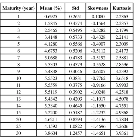
Table 2.1 provides summary statistics for the di¤erent maturity forward rates over the sample period. This table provides a benchmark for the level of forward rates and their standard deviations over the estimation period. Figure 2.1 plots the forward rates’time series evolutions. Interestingly, one can see a decline in the observed forward rates between 2008 and 2011, most pronounced for the 1, 2, 3, and 5 year forward rates.
Figure 2.2 graphs the evolution of the Fed’s balance sheet over the sample period.7 The Fed’s purchases mainly focused on mortgage-backed securities (MBS) during QE1 and Treasury securities during QE2. This di¤erence in the types of
5https://www.federalreserve.gov/econresdata/researchdata.htm
6We also explored the estimation using forward rates based on a polynomial spline smoothing procedure yielding similar results. For brevity these results are not reported in the subsequent text.
Maturity (year) Mean (%) Std Skewness Kurtosis 1 0.6925 0.2651 0.1080 2.2363 2 1.5845 0.4574 -0.1564 2.2357 3 2.5465 0.5495 -0.3282 2.1799 4 3.4148 0.5733 -0.4328 2.2141 5 4.1280 0.5566 -0.4907 2.3009 6 4.6753 0.5206 -0.5112 2.4173 7 5.0688 0.4783 -0.5192 2.5881 8 5.3303 0.4379 -0.5528 2.8596 9 5.4838 0.4046 -0.6407 3.2392 10 5.5523 0.3831 -0.7762 3.6518 11 5.5559 0.3775 -0.9166 3.9903 12 5.5119 0.3902 -1.0248 4.2518 13 5.4342 0.4203 -1.1017 4.5078 14 5.3340 0.4645 -1.1650 4.7551 15 5.2200 0.5187 -1.2232 4.9368 20 4.6211 0.8293 -1.4136 4.7804 25 4.1592 1.0822 -1.4696 4.2606 30 3.8604 1.2457 -1.4651 3.9361
Table 2.1: Summary Statistics
asset purchased across QE1 and QE2 suggests that there may be di¤ering price impacts. We explore this possibility in our estimation below.
Figure 2.3 provides a breakdown of the Fed’s Treasury holdings by maturity over our sample period. For their Treasury security purchases, the Fed’s activities are mostly concentrated on securities with maturities between one and ten years. These holdings will be relevant when discussing the QE’s impact on bond price yields in subsequent sections.
Relevant to the Fed’s Treasury purchases and their impact on forward rates is the outstanding supply of Treasury securities during the QE period. As mentioned earlier, we do not explicitly adjust our estimates of the Fed’s QE impact on forward rates for changes in the outstanding supply of Treasuries. In our methodology, this
Figure 2.3: Breakdown of Treasury Holdings by Maturity
supply adjustment is implicitly captured through its impact on the estimated true forward rate process (the drift and volatilities) over this time period. A potential concern with our methodology, therefore, is that if the U. S. Treasury purposely increased its auction of Treasuries to take advantage of the Fed’s QE activities, then our estimated price impacts would be biased low. To investigate this potential bias, Figure 2.4 shows the time series of newly auctioned Treasury securities over the QE period.8 As seen, the newly auctioned Treasuries are quite stable and only slightly increasing across time, the upward trend re‡ecting an increase in the size of the Federal budget de…cit over this same time period. It does not appear that the U.S. Treasury’s auction process was directly in‡uenced by the Fed’s QE activities, minimizing this potential bias in our estimation methodology.
Figure 2.4: Amount of Newly Auctioned Treasury Securities
2.2.2
A One-Factor Model
This section estimates a one-factor a¢ ne model for the evolution of the term structure of interest rates. We start with the one-factor model to both illustrate the methodology and to provide a benchmark for comparing the results for two-and three-factor models.
The Methodology
In the one-factor a¢ ne model, the true forward rates evolution given by expression (2.2) can be written as:
f(t; T) = (1 e k(T t)) 2 r 2k2 1 e k(T t) +e k(T t)r t (2.14)
where the state variable rt is the true instantaneous spot rate. Substitution into expression (2.7) gives the observed forward rate process, including the Fed’s price impact: F(t; T) (2.15) = 8 > > > > > > > < > > > > > > > : (1 e k(T t)) 2r 2k2 1 e k(T t) +e k(T t)rt (T(T))(1 e (T)t), if 0< t (1 e k(T t)) 2r 2k2 1 e k(T t) +e k(T t)r t (T) (T)(e (T) 1)e (T)t, if t > :
As mentioned previously, since the spot rate is unobservable9, to estimate our system we use a Kalman …lter. In our Kalman …lter, the time-discretized state transition equation for the spot rate is given by
rt+ t= (1 e k t) +e k trt+ r"t (2.16) where "t follows a standard normal distribution.
As indicated, this evolution allows the spot rate to be negative with positive probability. Although alternative evolutions could be used that preclude negative 9Instead, one could obtain estimated spot rates using the intercept of the smoothed GSW forward rate curve with the y-axis. We choose not to use these estimates because the intercept with the y-axis explicitly depends on the functional form of the smoothing function, which in turn, is greatly in‡uenced by the prices of the long-term Treasuries. In reality, short-term Treasury rates (less than one year) are in‡uenced more by the impact of the Fed’s short-term interest rate policies than the assumed shape of a smoothing function. Our estimation methodology avoids this potential bias.
rates, both economic theory and the empirical evidence are more consistent with evolutions that allow negative (nominal) rates with positive probability. Indeed, from a theoretical perspective, large …nancial institutions cannot store currency, they can only invest it in either deposits or securities; and consequently, negative rates are possible. Empirically, negative rates on Treasuries were observed in each of November 2009, June 2011, and August 2011;10 and the Bank of New York Mellon paid negative deposit rates in August 2011.11
For the Kalman …lter, the measurement equation is given by the evolution of the observed forward rate process:
F(t; i) = Ai+Birt+ut( i) (2.17) where Ai = 8 > < > : (1 e k i) 2r 2k2 1 e k i i i(1 e it), if 0< t (1 e k i) 2r 2k2 1 e k i i i(e i 1)e it, if t > (2.18) Bi = e k i, and i =Ti t:
For simplicity, we assumeut( i)follows an independent normal distribution. We estimate the parameters using three forward rate series ( i = 1yr; 2yr; 3yr). The parameters to be estimated are (k; ; r; 1; 1; 2; 2; 3; 3).
10See WSJ Blog, Market Beat, November 20, 2009, "Some Treasury Bill Rates Negative Again Friday;" Bloomberg, November 19, 2009, "U.S. 3-month Bills Turn Negative on Concern Risk Rally Overdone;" Bloomberg, June 27, 2011, "Treasury 4-week Bill Rates Negative for First Time since 2010;" WSJ Blog, Market Beat, August 4, 2011, "From One Crisis to Another: One Month T-Bill Yields go Negative Again."
11See Bloomberg.com/news, August 5, 2011, "BNY Mellon Makes Clients Pay for Deposits as Investors Seek Safety in Cash;" Online WSJ, August 5, 2011, "New Fee to Bank Cash."
Parameter Estimate Std θ 0.037 0.003 k 0.234 0.017 σr 0.013 0.001 λ1 2.20 0.29 λ2 1.28 0.21 λ3 0.0001 0.13 ψ1 0.053 0.008 ψ2 0.023 0.004 ψ3 0.0037 0.001
Table 2.2: One-Factor Parameter Estimates
Figure 2.5: One-factor Estimation of the Instantaneous Short Rate
The Results
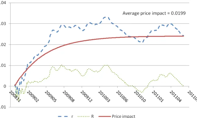
The parameter estimates are shown in Table 2.2 and the evolution of the true spot rate is plotted as the dashed curve in Figure 2.5.
The spot rate, with the Fed’s impact included, is the limit of expression (2.15) asT !t, i.e. Rt=rt 8 > < > : (0) (0)(1 e (0)t), if 0< t (0) (0)(e (0) 1)e (0)t, if t > :
To obtain an estimate of this spot rate, we use the estimates of( (1); (1))instead of( (0); (0)). The corresponding estimated short rate (denoted byRt) is plotted as the dotted curve in Figure 2.5. The di¤erence(rt Rt)is the Fed’s price impact, which is plotted as the solid curve. A positive and upward trending price impact curve in Figure 2.5 is consistent with the facts that the Fed’s monetary policy was targeting near zero short-term rates, and the Fed had been continuously purchasing Treasury securities over the estimation period. It shows that, under the one-factor model, the Fed’s price impact on the short rate has been increasing since QE started, and stayed in the range of2:3% 2:4% until the end of June 2011.
Table 2.2 presents the estimated price impact parameters for the one-, two-, and three- year forward rates ( i, i) for i = 1;2;3. The marginal impact parameter is decreasing in maturity, i.e. 1 > 2 > 3. In contrast, the mean reversion parameter is increasing with maturity, i.e. 1 > 2 > 3. This implies that the duration of the price impact increases with maturity. De…ning the half-life of the price impact as the time ti
0 = ln(2)= i for i = 1;2;3, then t10 = 0:32 3:8 months andt2
0 = 0:54 6:5months. The half life of the price impact of the 3-year forward rate is not de…ned since 3 is insigni…cantly di¤erent from zero.
These results can be best understood using the modi…ed expectations hypothe-sis that always holds in an arbitrage-free term structure model (see Jarrow (2009)). The expectations hypothesis is modi…ed for risk aversion using adjusted probabil-ities, instead of the actual probabilities.12 As in the classical expectations hypoth-12These adjusted probabilities are called the forward price martingale probability measures,
esis, except for this modi…cation, the time t forward rate for date T is the time
t "expected" spot rate for date T. These results show that the impact of QE on the future spot rate is "expected" to decline as time progresses. And in addition, the e¤ect of a purchase on the future spot rate is "expected" to last longer, the longer the term of the rate. Perhaps because most monetary policy activities occur on the very short-end of the curve, diminishing the lasting power of any quantity impact on the short-term forward rates.
2.2.3
An N-Factor Model
The above estimation procedure can be extended to a N - factor a¢ ne model, where the short rate is a sum ofN factors
r(t) = N
X
n=1
zn(t): (2.19)
Each factor zn(t) evolves as
dzn(t) =kn( n zn(t))dt+ ndWn(t) (2.20) where Wi(t) for i= 1; :::; N are independent standard Wiener processes.
Under this framework, one can show that the zero-coupon bond price is13
P(t; T) = exp ( C(t; T) N X n=1 Dn(t; T)zn(t) ) (2.21) where Dn(t; T) = 1 e kn(T t) kn C(t; T) = N X n=1 n T t+ e kn(T t) 1 kn : see Jarrow (2009).
13For the technical details, see Chapter 4 of Brigo and Mercurio (2006), Chapter 2 of Jeanblanc, Yor and Chesney (2009), and Bolder (2001).
The corresponding forward rates are F(t; T) = @lnP(t; T) @T = N X n=1 @Dn(t; T) @T zn(t) @C(t; T) @T = N X n=1 e kn(T t)z n(t) + N X n=1 n 1 e kn(T t) : (2.22) Therefore, the time-discretized state transition equation can be written as
zn(t+ t) = n(1 e kn t) +e kn tzn(t) +"n(t) n = 1; :::; N (2.23) where"n(t)follow zero-mean normal distributions with the following variance and covariance V ar["n(t)jFt t] = 2 n 2kn 1 e 2kn t Cov["n(t); "m(t)jFt t] = 0 n6=m
where Ft is the natural …ltration generated by the state variables process up to time t.
Recall that expression (2.7) describes the relation between the unobserved for-ward rates without the Fed’s impact (f(t; T)) and the observed forward rates with the Fed’s impact (F(t; T)). Combining expressions (2.7) and (2.22), we obtain the measurement equation: F(t; i) = Ai+ N X n=1 Bi;nzn(t) +ut( i) (2.24) where ut( i) are assumed to follow independent normal distributions,
Bi;n =e kn i, and i =Ti t: For 0< t , Ai = N X n=1 n 1 e kn i i i (1 e it):
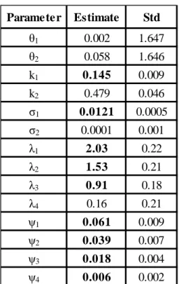
Paramete r Estimate Std θ1 0.002 1.647 θ2 0.058 1.646 k1 0.145 0.009 k2 0.479 0.046 σ1 0.0121 0.0005 σ2 0.0001 0.001 λ1 2.03 0.22 λ2 1.53 0.21 λ3 0.91 0.18 λ4 0.16 0.21 ψ1 0.061 0.009 ψ2 0.039 0.007 ψ3 0.018 0.004 ψ4 0.006 0.002
Table 2.3: Two-Factor Parameter Estimates For t > , Ai = N X n=1 n 1 e kn i i i (e i 1)e it: The Results
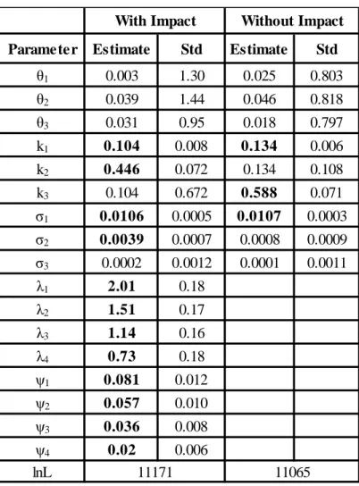
This section estimates both two- and three-factor models. We estimate the para-meters using four forward rates ( i = 1; 2; 3; 4 years). For the two-factor model, the parameters to be estimated are (ki, i, i, ( j, j)j=1;2;3;4)i=1;2 and the results are shown in Table 2.3. For the three-factor model, the parameters to be estimated are (ki, i, i, ( j, j)j=1;2;3;4)i=1;2;3 and the results are shown in Table 2.4. For comparison with the existing literature estimating a¢ ne models without Fed pur-chases, Table 2.4 provides the estimates for this model as well. These estimates without the Fed purchases included are consistent with those found in the existing
Paramete r Estimate Std Estimate Std θ1 0.003 1.30 0.025 0.803 θ2 0.039 1.44 0.046 0.818 θ3 0.031 0.95 0.018 0.797 k1 0.104 0.008 0.134 0.006 k2 0.446 0.072 0.134 0.108 k3 0.104 0.672 0.588 0.071 σ1 0.0106 0.0005 0.0107 0.0003 σ2 0.0039 0.0007 0.0008 0.0009 σ3 0.0002 0.0012 0.0001 0.0011 λ1 2.01 0.18 λ2 1.51 0.17 λ3 1.14 0.16 λ4 0.73 0.18 ψ1 0.081 0.012 ψ2 0.057 0.010 ψ3 0.036 0.008 ψ4 0.02 0.006 lnL
With Impact Without Impact
11171 11065
Table 2.4: Three-factor Parameter Estimates literature (see Babbs and Nowman (1999)).
The estimates of n (n = 1;2;3) have large standard errors because the ex-pression forAi reveals that the model has poor identi…cation for the individual n. However, i and i can be estimated with much higher precision.
Consistent with the results from the one-factor model, we …nd that the mag-nitude of the impact on the i- year forward rate becomes smaller as i gets larger ( j > i for j < i), while the impact on the i- year forward rate lasts longer for larger i (1= j < 1= i for j < i). The half-lives of the impact for the two-factor model ist10 = 0:34 4:1months, t20 = 0:45 5:4 months,t30 = 0:76 9:1months,
Parameter Estimate Std Half-life
(months) Parameter Estimate Std
λ1 2.01 0.18 4.1 ψ1 0.081 0.012 λ2 1.51 0.17 5.5 ψ2 0.057 0.01 λ3 1.14 0.16 7.3 ψ3 0.036 0.008 λ4 0.73 0.18 11.4 ψ4 0.020 0.006 λ5 0.69 0.10 12.1 ψ5 0.015 0.0013 λ6 0.48 0.11 17.3 ψ6 0.010 0.0011 λ7 0.52 0.11 16.0 ψ7 0.010 0.0012 λ8 0.62 0.14 13.4 ψ8 0.010 0.0017 λ9 0.85 0.11 9.8 ψ9 0.012 0.0015 λ10 1.06 0.16 7.8 ψ10 0.012 0.0019 λ11 1.70 0.14 4.9 ψ11 0.015 0.003 λ12 2.14 0.23 3.9 ψ12 0.016 0.0031 λ13 2.59 2.91 - ψ13 0.007 0.009 λ14 3.16 3.87 - ψ14 0.008 0.017
Table 2.5: Term Structure of the Fed’s Impact
and the half-lives of the three-factor model ist10 = 0:34 4:1months, t20 = 0:46 5:5 months, t30 = 0:61 7:3 months, t40 = 0:95 11:4 months. The fact that the two-factor and three-factor models give similar results shows the robustness of the estimation procedure.
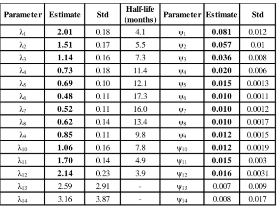
To determine the impact of the Fed’s QE program on long-term rates, Table 2.5 presents the Fed’s impact parameters estimated using a three-factor model for all maturity forward rates ranging from one to thirty years. This is the key Table of this chapter. These parameter estimates are obtained by …tting a three-factor model using the forward rates ( = 1; 2; 3; iyears) fori= 5; 6; ::: ;30where the parameters ( j, j)j=1;2;3 are …xed at their values given in Table 2.4. Hence, only the parameters (ki, i, i)i=1;2;3 and ( i, i) are reestimated where i corresponds to the longest term forward rate used in the estimation. This two-step procedure is invoked because there are too many parameters to estimate in the larger system
of equations, given the size of our data set.
As seen in Table 2.5, only the …rst 12 year forward rates’marginal price impact parameters ( , ) are signi…cantly di¤erent from zero. Because the impacts on rates beyond twelve years are all insigni…cantly di¤erent from zero, only the results for maturities less than 14 years are shown. A graphic representation of these estimates is given in Figure 2.6. The top panel plots the half-life of the impact for each maturity forward rate. These results show that the half-life increases as the maturity increases up to about 6 years, then declines thereafter. The lower panel plots the magnitudes of the marginal price impacts. They decrease monotonically as the maturity increases.
These results show that the Fed’s QE program a¤ects only short- and medium-term forward rates, up to about 12 years. After 12 years, the Fed’s QE program has no discernible e¤ect on forward rates. This is in contrast to the Fed’s stated intention of QE to a¤ect term rates. The absence of any impact on long-term forward rates is not surprising given that the Fed concentrated its Treasury purchases on maturities of less than 10 years (see Figure 2.3). Although there is a spill-over e¤ect on the 11- and 12- year maturity Treasuries, there is little if any spill-over on the 20 and 30 year bonds. If the Fed hopes to a¤ect the long-term forward rates, the evidence suggests that they need to purchase the long-term bonds directly.
This does not mean, however, that the Fed’s QE program does not a¤ect long-term bond yields. It does because long-long-term bond yields are an average of the forward rates over the bond’s life, and the Fed’s QE program has a large impact on short-term forward rates. The impact of the Fed’s QE program on bond yields is presented in a subsequent section.
Figure 2.6: Term Structure of the QE Impact
2.2.4
Separating QE1 and QE2
As mentioned earlier and shown in Figure 2.2, the Fed’s asset purchases di¤ered across QE1 and QE2. For this reason, it is likely that the price impact on Trea-suries di¤ered across these two periods. This section addresses this possibility by estimating the model’s parameters separately for each of the two time periods. To capture any information leakage, we choose the estimation periods for both QE events to start one day ahead of the o¢ cial announcement, i.e., the QE1 estimation period spans from November 24, 2008 to March 31, 2010, and the QE2 estimation period ranges from November 2, 2010 to June 30, 2011.
Figure 2.7: Impact of QE1
Due to the small sample size, estimating a three-factor a¢ ne model for each sub-period generates too large a set of sample errors and inconclusive results. Therefore, in order to get more reliable estimates, we …t a one-factor model. To justify this simpli…cation, we performed the analysis on only the short- to medium-section of the term structure, up to 8 years. A principal component analysis (PCA) using forward rates with maturities of less than eight years con…rms that the …rst principal component accounts for 93% of the variation, showing that a one-factor model provides a good approximation for this section of the term structure.
The estimation results for QE1 and QE2 are shown in Table 2.6 (Figure 2.7 and Figure 2.8 provide graphic views). Similar to the previous results obtained using the whole sample period (Table 2.5 and Figure 2.6), we …nd that the impacts
Parameter Estimate Std Half-life
(months) Parameter Estimate Std
λ1 2.13 0.76 3.9 ψ1 0.077 0.029 λ2 1.48 1.02 5.6 ψ2 0.042 0.017 λ3 0.61 0.58 13.6 ψ3 0.005 0.003 λ4 Large - 0 ψ4 0 -λ5 Large - 0 ψ5 0 -λ6 Large - 0 ψ6 0 -λ7 Large - 0 ψ7 0
-Panel A: QE1 Period
Parameter Estimate Std Half-life
(months) Parameter Estimate Std
λ1 3.25 0.81 2.6 ψ1 0.11 0.031 λ2 2.17 0.55 3.8 ψ2 0.065 0.011 λ3 0.65 0.54 12.8 ψ3 0.018 0.005 λ4 0.91 0.88 9.5 ψ4 0.003 0.001 λ5 Large - 0 ψ5 0 -λ6 Large - 0 ψ6 0 -λ7 Large - 0 ψ7 0
-Panel B: QE2 Period
Table 2.6: Term Structure of the Fed’s Impact
of both QE’s are limited to the one- to four- year forward rates. For maturities longer than four years, the estimates of the mean reversion parameter are denoted "Large" because in the numerical convergence procedure use for optimizing the likelihood function, the estimates always reach the pre-set upper bound, even when the upper bound is set at very large values (>50). Since the half-life is the inverse of , a large means that the price impact lasts for only a very short period.
Figure 2.8: Impact of QE2
instead of MBS and agencies as in QE1 (see Figure 2.2), we …nd that for maturities less than four years, QE2’s price impact on Treasury rates is larger than that of QE1. However, the duration of the impact lasts longer in QE1 than in QE2. For instance, QE1’s impact on the two-year rate lasts for5:6 months with magnitude of 4:2% per year, while QE2’s impact on the same rate lasts for 3:8 months with a magnitude of 6:5% per year. It is important to note that although the direct purchases of Treasury securities have a larger price impact on Treasury rates than do the purchases of MBS and agencies, the price impact on Treasuries of purchas-ing these alternative assets is signi…cant. These results con…rm the belief that asset substitution is an important e¤ect of Fed purchases in …xed income security markets (see Bernanke and Reinhart (2004)).
2.2.5
Test for Arbitrage
Given the parameter estimates from Table 2.5, we can test for the satisfaction of expression (2.12) to see whether the Fed’s QE Treasury purchases distorted risk premium and introduced arbitrage opportunities into the economy. Since the QE purchases only a¤ected forward rate maturities of less than or equal to 12 years, we only use these rates to test this proposition.
For the three-factor model, from expression (2.12), we have that 1(t; j) 1(t) + 2(t; j) 2(t) + 3(t; j) 3(t)
= ( j)e ( j)t for 0< t (2.25)
where n(t) = n(t) n(t)and ( j = 1; :::;12years).
To understand the intuition underlying our testing procedure, consider solv-ing expression (2.25) for ( 1(t); 2(t); 3(t)) using any three-tuple of dis-tinct maturity forward rates. In general, the solution for( 1(t); 2(t); 3(t)) will depend upon the particular forward rate maturities selected. Theorem 1 states that the evolution is arbitrage-free if and only if this is not the case, i.e. no matter which three-tuple of forward rates is selected, the same solution for ( 1(t); 2(t); 3(t))must occur. We test this observation below.
To formulate our test statistic, …x a timetin the QE time period, and letyjt = ( j)e ( j)t,xjt = ( 1(t; j); 2(t; j); 3(t; j))0, and t = ( 1(t); 2(t); 3(t)). Note that in this notation, we are assuming that tdoes not depend on the forward rate’s maturity. First, we estimate t using a simple linear regression
yjt = txjt+"jt f or j= 1; :::;12 (2.26) where"jtare assumed to bei:i:d:normal distributions with zero mean, representing
observational noise in the data.
If expression (2.25) is true, the null hypothesis, excluding the noise in the data we would expect to see"jt 0for allj. However, given noise in the data, we would expect to see var("jt)small relative tovar(yjt). To test this expectation, we form the test statisticst =P12j=1(yjt xjtbt)2=var(yjt)wherebtrepresents the regression estimate from expression (2.26). The test statistic st has a 2 distribution with 9 degrees of freedom (12 data points are used to estimate 3 parameters). If st is large, we can reject the null hypothesis of no arbitrage.
Estimating expression (2.26) for each day(t)over the sample period we obtain a time-series of the estimated market prices of risk bt, which are plotted in Panel A of Figure 2.9, and the test statistic, which is graphed in Panel B of Figure 2.9. As seen, the test statistic is well below the 5% signi…cance threshold. We can not reject the null hypothesis that there is no arbitrage over the QE period. As intended, the Fed’s QE program appears to have been successful in not introducing arbitrage opportunities into the economy. A quali…cation of our results needs to be noted. Since our parameters are estimated with smoothed Treasury price data, the smoothing procedure could itself remove arbitrage opportunitites, providing only a weak test of our hypothesis. A better test would involve using unsmoothed Treasury prices directly.
2.3
Model Speci…cation Tests
This section provides various model speci…cation tests that support the model’s validity.
Figure 2.9: Test for Arbitrage
2.3.1
A Comparison Pre- QE
To test the model’s speci…cation, we estimated the three-factor model for two time periods before the onset of QE1. One is from January 2, 2001 to August 1, 2003, when the Fed lowered interest rates, and the second from January 2, 2004 to August 1, 2006, when the Fed increased interest rates. If the additional structure in our model captures the Fed’s QE activities, one would expect to see the mean reversion and marginal impact parameters ( ; ) insigni…cantly di¤erent from zero during these time periods. The parameters are estimated using four forward rates ( i = 1; 2; 3; 4 years) and the results are presented in Tables 2.7 and 2.8.
para-Parameter Estimate Std Estimate Std θ1 0.021 0.82 0.023 0.82 θ2 0.02 0.82 0.029 0.82 θ3 0.022 0.82 0.024 0.82 k1 0.59 0.31 0.26 0.15 k2 0.28 0.06 0.25 0.02 k3 0.28 0.12 0.25 0.03 σ1 0.0001 0.015 0.005 0.009 σ2 0.032 0.009 0.026 0.005 σ3 0.016 0.007 0.021 0.005 λ1 1.35 0.62 λ2 0.75 0.64 λ3 0.35 0.71 λ4 0 0.9 ψ1 0.071 0.023 ψ2 0.035 0.015 ψ3 0.017 0.011 ψ4 0.008 0.008 lnL
With Impact Without Impact
9563 9508
Table 2.7: Robustness Check: Jan. 2, 2001 - Aug. 1, 2003
meters ( , ) are insigni…cantly di¤erent from zero, except for the price impacts of the one- and two- year rates. Although the one-year rate impact is signi…cant, its magnitude (0:071) is less than its magnitude (0:081) in the QE period (see Table 2.4). The same is true for the two-year rate. These impacts on the shortest term forward rates are consistent with the Fed’s direct monetary policy activities having a spill over e¤ect on the one- and two- year rates.
For the period when the Fed was increasing interest rates, all of the marginal impact parameters ( ) are insigni…cantly di¤erent from zero, except for the four-year rate. The mean reversion parameters ( ) are signi…cant for four-years two through
Parameter Estimate Std Estimate Std θ1 0.006 0.94 0.02 0.82 θ2 0.071 1.25 0.022 0.82 θ3 0.009 0.95 0.018 0.82 k1 0.45 0.08 0.98 0.06 k2 0.21 0.02 0.2 0.03 k3 0.21 0.04 0.2 0.03 σ1 0.0001 0.005 0.069 0.007 σ2 0.019 0.003 0.015 0.002 σ3 0.012 0.005 0.013 0.003 λ1 0.87 0.38 λ2 1.59 0.31 λ3 1.11 0.21 λ4 1.2 0.16 ψ1 -0.01 0.007 ψ2 0.0006 0.007 ψ3 0.01 0.005 ψ4 0.018 0.004 lnL
With Impact Without Impact
10738 10698
Table 2.8: Robustness Check: Jan. 2, 2004 - Aug. 1, 2006
four. The signi…cance for years two and three are irrelevant, since the market impact parameter is not di¤erent from zero. The signi…cance of both of the price impact parameters ( , ) for the four-year rate is probably due to noise in the data, but it could be due to the simplicity of the model being estimated. A resolution of these two possibilities awaits the estimation of more complex models in subsequent research.
2.3.2
Likelihood Ratio Tests, Pre- and Post- QE
This section provides likelihood ratio tests for the model with and without the Fed’s impact function for all three sample periods, both pre- and post- QE. These results are given in Tables 2.4, 2.7, and 2.8. The test statistic is2(ln(L1) ln(L2)), where L1 (L2) is the maximized likelihood value with (without) the price impact term.
At the 5% signi…cance level, the likelihood ratio test rejects the model without the price impact for all three sample periods. This is to be expected since this is an in sample test, and the price impact model has more parameters. More insightful is a comparison of the magnitudes of the changes in the likelihood values over the di¤erent sample periods. For the 1/2/2001-8/1/2003 sample (no QE), the log-likelihood increases by 0.6% after adding the price impact term. For the 1/2/2004-8/1/2006 (no QE) sample period, the increase is only 0.4%. In contrast, for the QE period, the log-likelihood increases the most, by 1%, after adding the price impact term. These relative changes in the likelihood ratio tests are consistent with the validity of the model.
2.3.3
Pricing Errors
Another way to test the model’s speci…cation is to study the model’s pricing errors in matching the observed forward rates. Table 2.9 presents the statistical properties of the forward rate errors for our three factor model (whose parameters are given in Table 2.4). Panel A shows the result for the model with the price impact term (call it the "adjusted model") and Panel B shows the result without the price impact term (call it the "conventional model").
Maturity (year) Mean (bp) SE t Skew Kurt ρ(1) ρ(10) ρ(20) 1 -2.10 0.75 -2.80 0.14 2.32 0.93 0.75 0.60 2 -3.97 0.73 -5.45 0.34 2.62 0.88 0.52 0.25 3 -2.30 1.07 -2.16 -0.24 2.61 0.94 0.71 0.50 4 -1.86 1.29 -1.44 -0.53 2.90 0.95 0.76 0.56 5 -1.59 1.44 -1.10 -0.55 2.88 0.97 0.76 0.56 6 0.49 1.47 0.34 -0.51 3.01 0.97 0.74 0.55 7 1.43 1.37 1.04 -0.32 3.19 0.96 0.71 0.50 8 1.29 1.31 0.98 -0.37 3.11 0.96 0.68 0.47 9 3.40 1.24 2.74 -0.47 3.02 0.96 0.67 0.45 10 1.01 1.23 0.82 -0.58 3.13 0.96 0.68 0.46 11 0.37 1.14 0.32 -0.57 2.92 0.96 0.66 0.43 12 -1.08 1.24 -0.87 -0.56 3.12 0.96 0.71 0.49 13 0.64 1.25 0.51 -0.51 2.71 0.96 0.71 0.51 14 -1.36 1.27 -1.07 -0.31 2.45 0.97 0.73 0.54 Panel A (With the price impact term)
Maturity (year) Mean (bp) SE t Skew Kurt ρ(1) ρ(10) ρ(20) 1 -3.84 0.71 -5.43 0.30 2.29 0.93 0.69 0.50 2 -15.08 0.83 -18.16 0.38 3.07 0.91 0.56 0.28 3 -6.14 1.28 -4.79 -0.13 2.31 0.96 0.76 0.56 4 4.84 1.50 3.24 -0.35 2.28 0.97 0.80 0.63 5 2.58 1.52 1.70 -0.43 2.41 0.97 0.79 0.62 6 -0.36 1.47 -0.24 -0.45 2.59 0.97 0.76 0.59 7 -1.96 1.40 -1.40 -0.45 2.81 0.97 0.73 0.55 8 -3.92 1.35 -2.91 -0.50 3.09 0.97 0.72 0.52 9 -3.00 1.32 -2.28 -0.60 3.40 0.97 0.71 0.51 10 -1.41 1.33 -1.06 -0.73 3.66 0.97 0.72 0.51 11 0.60 1.26 0.47 -0.66 3.24 0.96 0.73 0.53 12 -1.62 1.47 -1.10 -0.94 4.10 0.97 0.78 0.59 13 -0.89 1.61 -0.55 -1.03 4.37 0.98 0.82 0.66 14 -1.06 1.76 -0.60 -1.11 4.62 0.98 0.85 0.71
Panel B (Without the price impact term)
The pricing errors for the adjusted model (Panel A) are quite small, on the order of 2 basis points. Compared to Panel B, one can see that for maturities within …ve years, the average pricing errors estimated from the conventional model are signi…cantly larger than those from the adjusted model. For maturities longer than …ve years, the two models generate pricing errors with similar magnitudes. This evidence is consistent with the Fed’s price impact on long-term forward rates being small. The pricing errors for both models exhibit autocorrelations, perhaps indicating that a more complex model may provide a better …t.
It is important to note that these results are similar in magnitude to the pric-ing errors obtained in the 4-factor a¢ ne model estimated by Adrian, Crump and Moench (2012, Table 4), where instead of adding the Fed’s deterministic price im-pact component, one adds an additional Brownian motion random shock to the forward rate’s evolution. The ability of the deterministic price impact component to match the performance of an additional random factor lends credence to the validity of the model.
2.4
Comparison to Existing Literature
This section compares our price impact estimates with those in the existing empir-ical literature. The estimates in the existing empirempir-ical literature are summarized in Table 2.10, Panel A for …ve studies: D’Amico and King (2011), Gagnon, Raskin, Remache, and Sack (2010), Krishnamurthy and Vissing-Jorgensen (2011), Li and Wei (2012), and Meaning and Zhu (2011). The existing literature studies the price impact on bond yields for maturities ranging between 1 - 30 years. As seen, the estimated price impact is around 40 basis points for short-term rates (less than 5
Paper Eve nt Me thodology
1yr 2yr 3yr 5yr 10yr 30yr Event study (Cumulative response) -34 -91 Time-series regression -52 QE1 Event study (Cumulative response) -25 -39 -74 -107 -73 QE2 Event study (Cumulative response) -2 -8 -20 -30 -21 Stock effect -30 Flow effect Li and Wei (2012) QE1&2 Time-series estimation -100 Meaning and Zhu (2011) QE2 Panel regression
-21bp on the whole yield curve on average Krishnamurthy and Vissing-Jorgensen (2011) D’Amico and
King (2012) QE1 -3.5bp on the sector purchased Tre asury Yie ld Changes (bp)
Gagnon, Raskin, Remache, and
Sack (2010)
QE1
Panel A: Other Papers’Results
Event
1yr 2yr 5yr 10yr 30yr
-327 -26 -50 -70 -76
Treasury Yie ld Changes (bp) QE1 and QE2
Panel B: Our Results
Table 2.10: Comparison with Other Papers’Results
years), and 75 - 100 basis points for long-term yields (greater than 5 years). To make this comparison, we need to transform our estimated impacts on forward rates from the three-factor model in Table 5 to changes in bond yields.
This transformation is a multi-step process. First, we compute the changes in the true and observed constant maturity zero-coupon bond prices using expression
Figure 2.10: QE Impacts on Bond Yields
(2.10). Then, given these true and observed constant maturity zero-coupon bond prices, we compute the true constant maturity par-bond yields for bonds with maturities 2 - 30 years.14 These true par-bond yields give the coupon payments to use for computing the prices of the observed bonds, using the observed zero-coupon bond prices. Finally, from these observed bond prices, we can compute the observed yields. A comparison of the true par-bond yields with the observed yields generates the desired change in the Treasury yields due to the Fed’s QE activities. These yield changes are contained in Table 2.10, Panel B and graphed in Figure 2.10.
14A par bond yield is that coupon payment that makes a bond’s current price equal its face value ($100). We compute the true coupon bond’s par-bond yield using the true zero-coupon bond prices.
As seen, the average yield changes are 327, 26, 50, 70, and 76 basis points for the 1, 2, 5, 10, and 30 year bond yields. Except for the 1-year rate, our numbers are similar in magnitude to those in the previous literature. Our estimate for the 1-year rate is signi…cantly larger. As discussed previously, this di¤erence is due to the fact that our estimates include the impact of the Fed’s short-term interest rate monetary policy activity during the QE period.
2.5
Final Comments
This chapter proposes a new framework to analyze the price impact on the Treasury yield curve due to a central bank’s bond trading activities. To test the theory, we estimated an arbitrage-free a¢ ne term-structure model over the time period when the Federal Reserve conducted QE program from late 2008 to the middle of 2011. Our …ndings suggest that the QE program has generated signi…cant price impacts on the short to mid-term Treasury forward rates of up to 12 years. However, the impacts on long-term rates (beyond 12 years) appear to be insigni…cant. Long-term yield can still be a¤ected because yield is an geometric average of all the future forward rates.
Our model is simpli…ed to facilitate an analytic representation. It can be gen-eralized to incorporate a more complex process for the large trader impact and the term structure of interest rates. These extensions could be topics for future research.
CHAPTER 3
THE IMPACT OF QUANTITATIVE EASING ON FOREIGN EXCHANGE RATES
The Federal Reserve’s quantitative easing (QE) program between 2008 and 2011 has generated signi…cant impact across …nancial markets. Not only the bond markets but also the currency markets have been a¤ected. In this period, the U.S. dollar has depreciated signi…cantly against the Japanese yen (Figure 3.1). An important question here is how much of the dollar depreciation can be ascribed to QE. We attempt to address this question in this chapter.
A central monetary authority can impact the foreign exchange (FX) rates di-rectly by trading in the currency market or indidi-rectly by a¤ecting interest rates. Previous studies have found that direct currency market interventions have limited impact (see overview in Dominguez and Frankel (1993)). However, there have been few studies to examine the indirect channel, i.e., a¤ecting FX rates by a¤ecting interest rates. The Federal Reserve’s 2008-2011 QE program provides an ideal event to study this impact channel. Over this period, the U.S. dollar depreciated signi…cantly against the Japanese yen (Figure 3.1). The size of the Fed’s balance sheet increased dramatically. However, the size of the Bank of Japan’s (BOJ) balance sheet remained relatively stable since it had been cutting back from its quantitative easing from 2000 to 2005 (Figures 3.2 and 3.3). Due to this, one can focus on the impact caused by the Fed’s activities without worrying about those of the BOJ.
In addition to the Fed’s QE, there are several other possible explanations for the signi…cant appreciation of the yen. The …rst is a safe-haven e¤ect. There have been persistent current account surpluses in Japan. When the …nancial crisis hit the
Figure 3.1: Evolution of USD/JPY
global economy, risk-averse investors ‡ocked to yen-denominated assets and that increased demand for the yen. The second argument for the yen appreciation is that it is due to the unwinding of carry trades. At the end of 2008, the Fed lowered the target federal funds rate to almost zero, making the yen carry trade unpro…table. As a result, investors unwound their positions, pushing up the demand for the yen. Third, Japan’s economy has been signi…cantly a¤ected by the triple disaster
of the earthquake that occurred on March 11, 2011, and the subsequent tsunami and nuclear plant failures. Following this three-way catastrophe, the yen began to appreciate with the expectation of Japanese …rms�