CEP 14-07
Overaccumulation, Interest, and Prices
Christopher M. Gunn
July 2014
CARLETON ECONOMIC PAPERS
Department of Economics
1125 Colonel By Drive Ottawa, Ontario, Canada
OVERACCUMULATION, INTEREST
AND PRICES
Christopher M. Gunn
∗†Carleton University
July 10, 2014
AbstractAn emerging view of business cycles from the news-shock literature suggests that recessions may occur when agents depress their demand for new capital upon the realization that they have accumulated too much conditional on current infor-mation. In this paper I use a New Keynesian model with a financial accelerator to study the behaviour of interest and prices under both a “technology boom-bust” driven by changes in expectation about TFP, and a “credit boom-bust” driven by changes in expectations about the efficiency of the financial sector. While the two scenarios are similar in that they both lead to a run-up and then sharp drop-off in new capital and debt, I show that the behaviour of interest and prices depends crit-ically on the nature of the new-shock driving the overaccumulation. In particular, the boom-phase of the TFP boom-bust is characterized by below-trend inflation or deflation, whereas that of the credit boom-bust is characterized by above-trend but low inflation. In contrast, inflation falls below-trend in the bust phases of both. I show that consistent with results elsewhere in the literature, stricter inflation-targeting fails to pull the economy toward the efficient equilibrium during the boom phase of the TFP boom-bust. In contrast, stricter inflation targeting pushes the economy closer to the flexible-price response during the boom-phase of the credit
boom-bust. In both cases however,conditional on realization of overaccumulation,
inflation-targeting pulls the economy towards the flexible price equilibrium.
Keywords: expectations-driven business cycle, boom-bust, news shock, monetary
policy, overaccumulation, inflation, financial accelerator, Great Recession.
JEL Classification: E3, E44
∗This research was supported by a research grant from the Social Sciences and Humanities Research
Council (SSHRC) of Canada
1
Introduction
In a typical DSGE model of aggregate fluctuations, recessions are the result of “contrac-tionary” exogenous shocks to fundamentals, be they technological, financial, monetary or preference. Understanding the role of policy then in turn involves understanding how nominal and other variables of policy interest respond to such fundamental shocks for given policy regimes. Indeed in the wake of the crisis of the Great Recession, the DSGE literature has been on a sprint to identify which shock(s) drove the economy into re-cession, and then conditional on this, trying to understand whether policy helped or hindered the response.
In this paper I investigate the behaviour of interest and prices under an alternative view of recessions espoused by the news-shock literature related to the overaccumulation of capital. According to this view, recessions can result simply from agents’ realiza-tion that they accumulated too much capital during the boom-times of the past under “overly-optimistic” expectations about the improvement of some fundamental in the fu-ture1. In contrast to the conventional view, these recessions need not involve any realized contractionary shocks to fundamentals. Instead, changes in expectations emerge as an independent driver of aggregate fluctuations. Moreover, the bust is inextricably linked to the boom by the endogenous accumulation of capital. As a result, understanding pol-icy during such a boom-bust requires moving beyond simply understanding the impact on interest and prices of realized shocks to fundamentals that may separately cause a boom or bust, to understanding how changes in expectations alone impact these nominal variables over an entire boom-bust cycle.
To study this relation between the nominal side of the economy and the dynamics of expectations over a boom-bust cycle, I used a relatively standard New Keynesian model with variable capital and the financial accelerator mechanism of Bernanke et al. (1999). I then allow for news-shocks about two different types of disturbances - stochastic
1See Beaudry and Portier (2004), Christiano et al. (2008), Jaimovich and Rebelo (2009), Gunn and
Johri (2011) and Dupor and Mehkari (2013) for structural models that explore the imperfect information feature of news shocks to simulate recessions due to overaccumulation.
economy-wide TFP and a stochastic economy-wide element in the financial sector - as a way of investigating how altering the ultimate source of expectations impacts the path of expectations and thus nominal variable variables over the cycle, and also as a way of representing “technology” and “credit” as two distinct contexts thought to be a factor in business cycles in general, and the last two recessions in particular.
While there has been some work done to study the behaviour of interest and prices under changes in expectations about the future path of total factor productivity (TFP) such as that in Christiano et al. (2008), Barsky and Sims (2009), Christiano et al. (2011), Beaudry and Portier (2013b) and Jinnai (2013), there has been little work on understand-ing their behaviour in overaccumulations due to non-TFP news episodes2. Moreover even in real models that abstract from nominal variables and policy, relative to the depth of the literature for TFP-driven news episodes, that for non-TFP episodes is rather thin3.
Yet allowing for anticipation effects in other stochastic process beyond just TFP-driven news episodes allows us to think about how overaccumulation could play a role more generally in recessions where changes in neutral technology appear not to have been a dominant factor. For example, Gunn and Johri (2013a) show in a real model with flexible prices how the onset of the Great Recession could have been triggered by the overaccu-mulation of capital and debt under expectations about innovations in the financial sector that failed to materialize. Furthermore, studying the impact of both TFP and non-TFP news on the nominal economy in the same exercise helps isolate relative expected shocks themselves on these variables, holding constant the structural mechanisms in the model that catalyze the booms in the response to news.
The stochastic process for TFP enters into the model in a standard way, such that in the financial accelerator framework a realized shock to TFP increases the demand for capital by entrepreneurs, but at the same time, shifts out the economy’s resource constraint through the supply-effects of the shock. To model the stochastic element in the
2See also Gilchrist and Leahy (2002) who study the nominal impact of anticipated shocks to
produc-tivity that shares features with the news-shock literature.
3See Leeper et al. (2012), Guo et al. (2012), Zeev and Khan (2012), Gortz and Tsoukalas (2013),
Gunn and Johri (2013a), Gunn and Johri (2013b) and Christiano et al. (2014) for models with non-TFP related news.
financial sector, I include a stochastic element in the financial contract that parameterizes the monitoring cost as in Gunn and Johri (2013a) and Levin et al. (2004). Under this framework, a stochastic shock to this process results in a reduction in the cost of default, leading to an increase in demand for new capital by entrepreneurs for a given risk-free rate and credit spread. Thus while realized shocks in both the technology and credit episodes lead to a direct increase in demand for capital, only in the TFP case does the shock also induce direct supply-side effects. As I will discuss later, this distinction between the expected effect of the two shock in a news framework has important consequences for the nominal side of the economy.
I allow for anticipation in both stochastic processes in a standard way as in Jaimovich and Rebelo (2009) and Christiano et al. (2008) such that news shocks in each respective stochastic process serve as imperfect signals about the future stochastic innovations. In both the TFP and credit episodes, news about an improvement in the respective stochas-tic process leads to an expansion of debt and capital in the present in anstochas-ticipation of the future. If in the future the news turns out to be ex-post incorrect, agents realize they have accumulated too much debt and capital, and as a result, depress their demand for new capital, leading the economy into recession driven by overaccumulation, scenarios that I refer to as “technology boom-bust” and “credit boom-bust” respectively. Interestingly, on the real side of the economy, the behaviour of real quantities and relative prices in
both the technology and credit boom-busts is nearly identical: consumption, investment, hours and output boom in response to good news, asset prices rise, and credit spreads fall. During the bust phase, the direction of these variables are reversed, although the recessionary response is much more sudden since the accumulated debt and capital along with revised expectations reflecting no changes in fundamentals means that entrepreneurs suddenly find themselves in poor financial health. Yet the behaviour of the nominal side of the economy in the two episodes diverges: in the technology boom-bust inflation is below-trend during both the boom and bust, whereas in the credit boom-bust inflation is above-trend yet low during the boom, and below-trend during the bust. Thus comparing the ex-post time-series of the two episodes, we see two very similar boom-busts in the
real economy in the absence of any variation in fundamentals, but a path of policy and inflation that is very different.
To understand the behaviour of the nominal side of the economy under such an over-accumulation boom-bust, consider that in a New Keynesian framework with standard sticky price mechanism such as Calvo-pricing, inflation is a function of current and ex-pected future marginal costs. The pre-shock boom-phase of such a news-driven cycle occurs in the absence of shocks to exogenous fundamentals, and is often described as be-ing akin to a demand-like shock if the change in expectations about the future translates into an increase in consumption and/or investment demand in the present leading to a dominant increase in the demand for goods in the present.4 Under a standard sticky-price framework, on average the production sector meets this change in demand with increased production in the present, driving up marginal costs in the present and thus putting upward pressure on inflation. Yet price-setters also look forward to the expected path of marginal costs beyond the pre-shock boom phase to the period when the shock is expected to hit. The response of inflation in the present will as a result depend on the behaviour of marginal costs in both the demand-driven pre-shock boom phase we well as the shock phase when the exogenous shock to fundamentals is expected to hit. Thus despite the fact that two distinct news shocks about different stochastic processes might cause a similar upward pressure on marginal costs in the initial demand-like boom phase of each respective episode, the response of initial inflation in each case may be different if the expected impact on marginal costs is different for when each respective shock hits in the future. As others such as Christiano et al. (2011) and Barsky and Sims (2009) have noted, shocks to TFP tend to exert downward pressure on marginal costs. If agents re-ceive news that TFP will rise in the future, forward-looking price-setters may as a result drop prices upon receipt of news if the expected drop in marginal costs in the future when the shock hits dominates the rise in marginal costs during the pre-shock boom. Indeed I
4Note that this statement is very model-dependent since it is reliant on the particular structural
mechanism driving the news boom. For example, in some models changes in expectations about the future may induce mechanisms which endogenously shift marginal costs downwards in the present, mimicking a supply-type effect.
show that the simulations of the TFP-driven news boom for the calibration in this paper yield a fall in inflation during the boom phase, consistent with predictions elsewhere in the literature using different structural models. In contrast to the TFP episode, in the credit episode agents expect that when the credit shock hits in the future it will lead to an increase the demand for capital, but without the supply-effects of the TFP shock that would otherwise put downward pressure on marginal costs in the future. Agents thus expect that the future credit shock will lead to a rise in marginal costs in the future, and as a result of this and the upward pressure on marginal costs in the boom phase, prices rise in the present. In the bust phases of both, the realization of overaccumulation of debt and capital leads to a sharp drop in the demand for new capital. Moreover, since in both cases the expected future path of fundamentals is no longer perturbed from steady-state, the impact of the drop in demand is similar for both episodes, leading to a drop in marginal costs and inflation that falls below steady state.
That TFP-driven news booms tend to predict low inflation or deflation when the real economy and asset prices boom is generally viewed as being consistent with evidence discussed by Christiano et al. (2008), Beaudry and Portier (2013b), Christiano et al. (2011) and Jinnai (2013) that in the data inflation tend to be lower during asset price booms. It would seem then that at least with this feature of the data, boom-busts associated with non-supply fundamental shocks such as a credit boom-bust would have the odds stacked against them: changes in expectations about shocks whose primary effect is to cause an increase in demand for capital and thus associated rise in marginal costs when the shock hits might be characterized by high inflation during the boom phase as price settings raise prices in the present to cover high future expected marginal costs in the futre as well as high marginal costs in the present. I demonstrate however that inflation remains low during the credit boom. This is driven partly by the presence of structural features such as capacity utilization which impair the rise in marginal costs, but also partly by the fact that only a portion of the overall credit boom is driven by inefficiencies introduced by sticky prices. In particular, in the same model under perfectly flexible prices, output still booms in response to news of the credit shock. Adding sticky
prices amplifies the boom by expanding the output gap relative to output under flexible prices, but this expansion in the output gap represents only a fraction of the overall variation in output. An implication of this is that from the perspective of the model, one cannot simply confront the data assuming that all of the cyclical variation in output in the data is driven purely by variation in the output gap. This result lies in contrast with results of New Keynesian models where news-booms are driven primarily by the inefficient response of the sticky price economy interacting with a sub-optimal monetary policy rule, such that in the illustrations provided in Beaudry and Portier (2013b) and Beaudry and Portier (2013a). Those models imply that all or most of the variation in observed output is driven by variation in the output gap itself. As such, from the perspective of those models, it is appropriate to assume that all of the observed variation in output is comprised of variation in the output gap. As Beaudry and Portier (2013b) note, when doing so, these models tend to imply inflation that is too volatile relative to output. This property also allows the model to offer a different perspective on criticisms that New Keynesian interpretations of the Great Recession tend to imply overly-volatile inflation relative to output, since these criticisms typically assume demand-shocks where much of the observed variation in output is comprised of variation in the output gap itself.
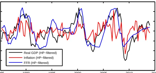
Can taking an overaccumulation view offer insight on the behaviour of interest and prices in the last two recessions? In the data we see a very different behaviour of prices and policy over the technology boom-bust of the late 1990’s and the credit boom-bust of the 2000’s, both of which involved a massive boom-bust in asset prices. Figure 1 shows that cyclically adjusted inflation was low during both the boom and bust of the late 1990’s, consistent with the predictions of the “technology” boom-bust provided by this model, but that inflation was above-trend yet low during the credit boom of the mid-2000’s, and then below trend at the start of the recession in 2009, both of which are consistent with the “credit boom-bust” predictions of the model. Thus despite the different path of prices and policy between these two boom-busts, the general notion of “overaccumulation” can account for them when we expand the set of fundamentals
1985 1990 1995 2000 2005 2010 2015 −4 −3 −2 −1 0 1 2 3 Real GDP (HP−filtered) Inflation (HP−filtered) FFR (HP−filtered)
Figure 1: Interest and prices over three recessions (U.S.).
driving changes in expectations beyond TFP.
Given the relation between expectations and marginal costs in the model, it is then important to understand how changing the stance of monetary policy impacts the nature of the boom-bust. Since shocks to TFP put downward pressure on inflation in this economy, a more vigilant central bank focused solely on inflation-targeting will lower the policy rate in order to stimulate inflation when TFP increases, with the consequence of amplifying the demand for new capital. In contrast, the inflationary impact of the credit shock implies that stricter inflation-targeting will suppress the demand for capital as the central banks leans against the effect of a fall in default costs. Thus looking forward from the boom pre-shock phase, in the TFP case agents anticipate that the bank’s actions will amplify the boom, whereas in the credit case they anticipate the bank will suppress it. Through simulation I show that consistent with results elsewhere in the literature, stricter inflation-targeting fails to pull the economy toward the flexible price equilibrium during the boom phase of the TFP boom-bust, whereas stricter inflation targeting pushes the economy closer to the flexible-price response during the phase of the credit boom-bust. In both cases however, conditional on realization of overaccumulation, inflation-targeting pulls the economy towards the flexible price equilibrium, since this phase is driven primarly by negative demand-like effect of the drop in demand for new capital.
The remainder of the paper proceeds as follows. In the next Section I present the model economy and then in Section 3 I discuss the parameterization. In Section 4 I discuss the behaviour of marginal costs and inflation implied by models of news, and then show the model implications through simulation for the technology boom-bust and TFP boom-bust. Following this I then perform various experiments where I vary the baseline policy rule to illustrate the impact of policy on the model. Section 5 concludes.
2
Model
The model economy is a standard New Keynesian framework with variable capital and a financial accelerator mechanism of Bernanke, Gertler and Gilchrist (1999). In addition, the borrowing and lending arrangement includes a stochastic process as in Gunn and Johri (2013a) that serves as the sources of credit news in the model credit boom-busts.
The economy consists of a continuum of identical households, a single final goods firm that nonetheless acts competitively, a continuum of monopolistically competitive intermediate goods firms indexed byj ∈[0,1], with each jth firm producing a differenti-ated good, one each of a capital-producer and financial intermediary who all nonetheless act competitively, and as well as a continuum of risk-neutral entrepreneurs indexed by i ∈ [0,1]. Households own goods-producers and capital-producer as well as the finan-cial intermediary. The intermediate goods firms produce output with labor and capital services, paying wages to households and renting capital services from entrepreneurs. En-trepreneurs purchase capital from the capital producer, financing their capital with their own wealth as well as from loans from the financial intermediary. The entrepreneurs’ capital returns are subject to idiosyncratic shocks observable to the entrepreneurs but not the financial intermediary, and thus the lending arrangement between the financial intermediary and a given entrepreneur involves agency costs. The financial intermedi-ary finances its loans to entrepreneurs by issuing risk-free securities to households. The capital-producer creates new capital by purchasing output from the goods market and combining it with existing capital. Nominal elements of the model enter in a cashless
manner as in Bernanke, Gertler and Gilchrist (1999). Nominal price rigidities are based on a Calvo pricing mechanism, but nominal wages are fully-flexible. Monetary policy consists of a Taylor-form nominal interest rate rule.
The model economy includes markets for final and intermediate goods, labour, house-hold deposits (financial securities), nominal bonds, intermediated loans, capital services, and capital goods.
2.1
Household
A typical household has preferences defined over sequences of consumptionCtand
hours-worked Nt with expected lifetime utility defined as
U =E0
∞
X
t=0
βtU(Ct, Nt), (1)
where β is the household’s subjective discount factor and the period utility function U(Ct, Nt) follows the class of preferences described in King, Plosser and Rebelo (1988),
and where for notational simplicity I abstract from indexing individual household vari-ables.
The household enters into each period with real financial securities At and nominal
bonds Bn
t, earning risk-free gross real rate of return Rta and risk-free gross nominal rate
of return Rn
t respectively, receiving nominal wage Wt for supplying hours Nt to the
goods-producing firms, and receiving a share of real profits from the capital-producers, goods-producers and financial intermediary, denoted collectively asFt. At the end of the
period, the household chooses its consumption Ct and its holdings of financial securities
At+1 to deposit with the financial intermediary.
The household’s period t budget constraint is given by
Ct+At+1+ Bn t+1 Pt =RatAt+Rtn Bn t Pt + Wt Pt Nt+Ft, (2)
central bank.
The household’s problem is to choose sequences of Ct,Nt,At+1 andBtn+1 to maximize
(1) subject to (2).
2.2
Final goods firm
The final goods firm produces the final goodYt by combining intermediate goodsyjt, j ∈
[0,1] according to the technology
Yt= Z 1 0 yjνdj 1ν , (3)
whereν∈(0,1] determines the elasticity of substitution between the intermediate goods. The producer acquires each jth intermediate good at pricePjt, and sells the final good into
the final goods market at pricePt where it may be used as a consumption or investment
good. Each period the producer chooses its demand for each intermediate good yjt by
maximizing its profits given by
PtYt−
Z 1
0
Pjtyjtdj. (4)
The resulting optimality condition then yields a demand function for the ith good as
yjt = Pjt Pt ν−11 Yt. (5)
2.3
Intermediate goods firms
Intermediate goodyjtis produced by an imperfect competitor according to the technology
technology
yjt =ztn˜αjt˜k
1−α
jt , (6)
wherezt is total factor productivity, ˜njt is total hours-worked, and ˜kjt is physical capital
that ˜ njt =nΩjt(n e jt) 1−Ω , (7)
where household labor njt is acquired at wage-rate wt and entrepreneurial labor nejt is
acquired at wage-rate we
t. Capital services ˜kjt is rented from entrepreneurs in capital
services markets at the rental ratert, and is defined by ˜kjt =ujtkit, wherekjt is the stock
of physical capital andujtis the utilization rate of that stock, chosen by the entrepreneurs.
The firm sells its output into the goods market at price Pjt.
Intermediate goods firms face Calvo frictions in setting their prices such that each period a fraction ζp of firms cannot optimize their price. A firm that is not able to
re-optimize in periodtits price in a given period continues to sell its output forPjt =Pjt−1.
A firm that can re-optimize its price in period t chooses its price Pjt∗ to solve
Et ∞ X s=0 ζpsβsλt+s λt Pjt∗yjt+s−Pt+sS(yjt+s) , (8)
given the production technology (6) and the demand curve (5), and where S(yjt) is the
firm’s real cost function as a solution to its cost-minimization problem for a given level of output yjt. The pricing problem results in the standard price-setting condition whereby
the forward-looking price-setters adjust prices in the present to reflected expected future marginal costs to account for the future contingencies where they will not have the opportunity to re-optimize their price.
2.4
Financial Intermediary
At the end of each period t the financial intermediary makes a portfolio of loans to the measure of entrepreneurs, with Bit+1 denoting the loan to the ith entrepreneur, funding
this portfolio of loans by issuing securities, At+1, to the household that promise a
risk-free gross return, Rat+1. The financial intermediary has no other sources of funds, and thus it must generate a total return on its loan portfolio in each aggregate contingency to just cover its opportunity cost of funds on the household securities. As in Bernanke
et al. (1999), each risk-neutral entrepreneur bears all the aggregate risk on its loan and thus makes state-contingent loan payments that ensure that in each aggregate state of the world the financial intermediary achieves an expected return equal to its opportunity cost of funds. This leaves the intermediary with only the idiosyncratic risk associated with individual loans, which it can diversify away by virtue of holding a large loan portfolio.
2.5
Entrepreneurs
Risk-neutral entrepreneurs accumulate physical capital and as well they make the ca-pacity utilization decisions for their capital as in Christiano et al. (2003). Relative to Gunn and Johri (2013a), the entrepreneurial framework is the same with the exception of modifications necessary to incorporate the capacity utilization. The timing of the decisions of the ith entrepreneur is as follows. The entrepreneur enters into period t with predetermined capital stock Kit, purchased at the end of the previous period from
capital producers for price qt−1, as well as debt obligations Bit. After observing the
ag-gregate state in period t, the entrepreneur chooses the capital utilization rate uit and
then rents capital services ˜Kit =uitKit at rental ratertto intermediate goods firms. The
entrepreneur then sells its entire capital stock to capital-goods producers for price ¯qt,
realizing its ex-post return to that capital, Rk
it, given by Rkit=ωit uitrt−a(uit) + ¯qt qt−1 . (9)
In the above expression, ωi is a random variable providing an idiosyncratic component
to entrepreneur i’s return, such that the ex-ante return to capital is subject to both idiosyncratic and aggregate risk. The random variableωis i.i.d across firms and time, has cumulative distribution functionF(ω), and is normalized so thatEω= 1. Note that the entrepreneur observes this idiosyncratic component when realizing its return, but after making its capacity utilization decision. As in Christiano et al. (2003), entrepreneurs incur a cost a(uit) per unit of capital in terms of goods for utilization rate uit, where
capital as in (9).
After realizing its return, the entrepreneur makes any necessary payments to the financial intermediary to fulfill the terms of its contract with financial intermediaries determined the previous period.
Finally at the end of the period, the entrepreneur chooses its desired level of capital, Kit+1, to hold into the following period, buying it from the capital producer for priceqt.
Entrepreneurs finance these capital purchases with their own end-of-period net-worth, Xit+1, and new loans from the financial intermediary Bit+1, such that their financing
satisfies
qtKit+1 =Xit+1+Bit+1. (10)
As in Bernanke et al. (1999), to prevent entrepreneurs from self-financing and elim-inating the need for external finance in the long run, the entrepreneur faces a constant probability, γ, of surviving into the next period. When entrepreneurs die they consume their entrepreneurial equity, ce
it. Finally, entrepreneurs supply a unit time endowment
inelastically to the good-producers at wage-ratewe t.
2.6
Agency problem and debt-contract
The agency problem and debt contract follows that of Bernanke et al. (1999), with modifications described in detail in Gunn and Johri (2013a) to account for a stochastic element. I describe the main elements here briefly and leave the details to the appendix.5 As indicated earlier, a given entrepreneur finances its desired level of capital to hold into next period partly with its own net-worth and partly with external financing from the financial intermediary. In describing the following contract for this external financing, I take the entrepreneur’s desired choice of capital Kit+1 as given, leaving discussion of the
entrepreneur’s capital utilization decision for the following section.
The financial intermediary can observe the average return to capital Rk
t but not
an entrepreneur’s idiosyncratic component ωit, unless it pays a monitoring cost. As a
consequence the parties can adopt a financial contract that minimizes the expected agency costs, in the form of risky-debt where the monitoring costs are incurred only in states where an entrepreneur fails to make promised debt payments. We can thus interpret this monitoring cost as a “default cost”. As in Bernanke et al. (1999) these default costs take the form of a fraction,θt, of the entrepreneur’s gross payout,ωitRktqt−1Kit, however,
unlike Bernanke et al. (1999), here θt is time-varying and follows a stochastic process,
common to all entrepreneurs, and observable by all agents in the economy.
At the end of period t, the entrepreneur chooses its capital expenditures,qtKit+1 and
associated level of borrowing, Bit+1, with knowledge of neither the aggregate state in
period t + 1 nor the idiosyncratic realization of ω in period t+ 1, ωit+1. Conditional
on these choices, the terms of the contract between the financial intermediary and the entrepreneur specify a contractual non-default state-contingent gross interest rate, Rl
it+1
that ensures that in each aggregate state of the world, the financial intermediary achieves an expected return equal to the its opportunity cost of funds. In the event that the entrepreneur’s idiosyncratic returns are insufficient to cover its contracted debt payments, the entrepreneur defaults and goes bankrupt, handing over all remaining gross returns to the financial intermediary, leaving the gross returns less default costs to the financial intermediary. Note that given the state-contingent contract structure, the loan rateRl
t(i)
will adjust in period t to reflect the ex-post realization of the aggregate state in t. I show in the appendix that such a contract results in the condition
[Γ(¯ωit+1)−θt+1G(¯ωit+1)]Rkt+1qtKit+1 =Rat+1(qtKit+1−Xit+1), (11)
where ¯ωit+1 is a “cut-off” level of ωit, defined by,
¯
where Γ(¯ω) is the financial intermediary’s expected share of gross returns, given by Γ(¯ωit) = [1−F(¯ωit)]¯ωit+ Z ω¯it 0 ωdF(ω), (13) and G(¯ω) is given by G(¯ωit) = Z ω¯it 0 ωdF(ω). (14)
The above condition (11) defines a menu of contracts for a given level of net-worth Xit+1 relating the entrepreneur’s choice of Kit+1 to the cut-off level of ¯ωit+1.
2.7
Entrepreneur’s problem
In this section I describe the entrepreneur’s capital utilization, capital stock and cut-off decisions.
2.7.1 Capacity utilization decision
The ith entrepreneur’s gross return in period t, after realization of the aggregate state but before the resolution of idiosyncratic risk, is given by
Vitk = Z ∞ ¯ ωit ωRktqt−1KitdF(ω)−RlitBit = Z ∞ ¯ ωit ω uitrt−a(uit) + ¯qt qt−1 qt−1KitdF(ω)−RitlBit. (15)
Noting that with the exception of uit, since all entrepreneurial-indexed variables are
predetermined at the timing juncture of the utilization decision, we can simply represent the risk-neutral entrepreneur’s choice of capacity utilization uit as the solution to the
problem
maxuituitrt−a(uit), (16)
yielding the first-order condition
2.7.2 Capital stock and cut-off decision
The entrepreneur’s expected gross return, conditional on the ex-post realization of the aggregate state but before the resolution of idiosyncratic risk, is given by
Vitk+1 = Z ∞ ¯ ωit+1 ωRkt+1qtKit+1dF(ω)−Rlit+1Bit+1, (18) which simplifies as Vitk+1 = [1−Γ(¯ωit+1]Rkt+1qtKit+1, (19)
where 1−Γ(¯ωit+1) is the entrepreneur’s expected share of gross returns.
For a given level of net-worth Xit+1, the risk-neutral entrepreneur’s optimal capital
and loan cut-off is then
maxKit+1,ω¯it+1Et{V
k
it+1}, (20)
subject to the condition that the financial intermediary’s expected return on the contract equal its opportunity cost of its borrowing, equation (11). Letting λit+1 be the ex-post
value of the Lagrange multiplier conditional on realization of the aggregate state, the first-order conditions are then
Γ0(¯ωit+1)−λt+1[Γ0(¯ωit+1)−θt+1G0(¯ωit+1)] = 0 (21) Et [1−Γ(¯ωit+1)] Rk t+1 Ra t+1 +λt+1 [Γ(¯ωit+1)−θt+1G(¯ωit+1)] Rk t+1 Ra t+1 −1 = 0 (22) [Γ(¯ωit+1)−θt+1G(¯ωit+1)]Rkit+1qtKit+1−Rat+1(qtKit+1−Xit+1) = 0, (23)
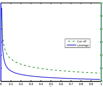
where (21) and (23) hold in each contingency, but (22) holds only in expectation. For constantθas in Bernanke et al. (1999), the above equations collapse into Bernanke et al. (1999)’s well-known result that the external finance premium RRk is proportional to the leverage of the entrepreneur. Introducing the time-varying cost of defaultθtas in the
conditions above then effectively introduces a dynamic wedge into this static relation. For example, given a fall inθ, the cost of default is now less, implying that a lending contract
0 0.1 0.2 0.3 0.4 0.5 0.6 0.7 0.8 0.9 1 1.5 2 2.5 3 3.5 4 4.5 θ Leverage 0 0.1 0.2 0.3 0.4 0.5 0.6 0.7 0.8 0.9 10.3 0.4 0.5 0.6 0.7 0.8 0.9 Cut−off ω Cut−off Leverage
Figure 2: Optimal contract: leverage (L) & cut-off (¯ω) vs. default cost (θ) holding the external finance premium (RRk) constant.
can now accommodate a higher level of leverage for a given external finance premium. In effect, changes in θ shift the menu of contracts that describe the combinations of cut-off and leverage consistent with the terms of the contract. Figure 2 shows the effect of varying θ on both the cut-off and leverage consistent with the contract for a given external finance premium Rk/Ra. Note that a fall inθ permits a higher level of leverage to satisfy the contract.
From the perspective of this paper, what is important from the above discussion is that a fall in the cost of defaultθcauses a rise in the demand for new capital by entrepreneurs for a given risk-free rate, since given the entrepreneur’s current net-worth, higher leverage allows a higher level of capital to fulfill contract conditions. Importantly, this rise in the demand for new capital occurs without any shift in the economy production possibilities frontier as would occur with a positive TFP shock zt. Instead, in this New Keynesian
framework, this increase in demand for investment must be met with either a reduction in consumption demand, and/or an increase in the supply of goods due to shifts in labour supply, labour demand and increased capacity utilization.
2.8
Capital-producer
The competitive capital-goods producer operates a within-period technology that com-bines existing capital with new goods to create new installed capital. At the end of each period it purchases existing capital Kk
t from entrepreneurs at price ¯qt, combining it with
investment It purchased from the goods market to yield new capital stock Ktnk, which
it sells back to entrepreneurs in the same period at price qt. The capital-producer faces
adjustment costs in the creation of new capital, and incurs depreciation in the process, so that
Ktnk = (1−δ)Ktk+ Φ( It Kk
t
)Ktk. (24)
The capital-goods producer chooses Knk
t , Ktk and It to maximize profits Πkt = qtKtnk −
¯
qtKtk−It, leading to the first-order conditions
qt= 1 Φ0( It Kk t ) (25) ¯ qt=qt (1−δ) + Φ( It Kk t ) − It Kt . (26)
2.9
Stochastic process
θ
tBoth TFPztand default costsθtfollow stationary stochastic processes that include news
shocks as imperfect signals about future innovations. I model the respective news shocks using a simple stylized formulation similar to that of Christiano et al. (2008), whereby agents receive news about the innovation p periods in advance. The news shocks are imperfect since in addition to the news signals, there is also an unanticipated shock for each process such that the innovation in any given period is the sum of an unanticipated and anticipated component. As such the stochastic process zt and θ evolve respectively
as
lnθt=ρθlnθt−1+θt−p+ε θ
and
lnzt=ρzlnzt−1+zt−p+ε z
t, (28)
where ρθ, ρz <1, θt−p and zt−p are news shocks that agents receive in periodt−p about
the innovation in t, and εθ
t and εzt are unanticipated shocks. All shocks are mean zero
and uncorrelated over time and with each other. Each shock has standard deviation σi,
where i={ρ, z, ερ, εz}.
Using these formulations, we can then think about scenarios where the unanticipated signals partially or fully offset the anticipated signals. For illustrative purposes it is helpful to consider the extreme fully unrealized case where the unanticipated shock in a given period fully offsets the anticipated shock such that the summation of the innovations is zero, given by εθ
t =−θt−p andεzt =−zt−p. In what follows, I refer to these cases as the
“credit boom-bust” and “technology boom-bust” respectively. It should be clear however that the analysis of the paper extends more generally beyond the full-offset case to cases where there is partial offset, such that an overaccumulation bust would correspond to a situation where the realization of some shock falls short of its expected realization.
2.10
Monetary policy
Monetary policy takes the form of a monetary authority that sets the gross nominal interest rate Rtn+1 according to a rule in the form
Rn t+1 Rn = Rn t Rn ρR" Πt Π φπ Yt Y∗ t φy#1−ρR , (29)
where variables without subscripts are steady-state values, Πt is the gross inflation rate,
and Yt
Yt∗ is the output gap, where Y ∗
3
Solution and parameterization
The model equilibrium is given in the appendix. I solve the resulting non-linear system by taking a linear approximation around the steady state. The model calibration for the real side of the economy is based on that of Gunn and Johri (2013a), where the parameters related to the financial accelerator are in turn based on those in Bernanke et al. (1999). As such I discuss the parameterization of the real side only briefly and refer to Gunn and Johri (2013a) for more detail. The parameterization for the nominal side of the economy is based on standard values used in the New Keynesian literature which I will discuss below.
Beginning with the parameters common to standard real-business cycle models, I set the household’s subjective discount factor β to 0.99, the share of labor in intermedi-ate goods production α = .67, depreciation of physical capital δ to 0.025, steady state utilization to uss = 1, and the elasticity of marginal utilization u = 0.25.
To promote comovement, I use preferences of the form used by King and Rebelo (2000) where the stand-in representative agent has the preference specification
u(Ct, Nt) = 1 1−σ Ct1−συ∗(Nt)1−σ−1 , (30) where υ∗(Nt) = h Nt H υ 1−σ σ 1 + 1− NHt υ 1−σ σ 2 i1−σσ
, where H is the fixed shift length, and υ1 and υ2 are constants representing the leisure component of utility of the underlying
employed group (who work H hours) and unemployed group (who work zero hours) respectively. For σ >1 these preferences are not separable in consumption and leisure. I set the fraction of the population working on average,fw to 0.6, the average household’s
share of time allocated to market work Nss to 0.3, and σ = 2 as in Gunn and Johri
(2013a).
The parameters associated with the financial contract and the entrepreneur follow Bernanke et al. (1999), such that in steady state, the external finance spreadRk−RA= 0.005, leverage, K/X, is approximately 2, and the fraction of entrepreneurs defaulting
each quarter is 0.076. The quarterly survival rate of entrepreneurs to 0.9795, the variance of log ¯ω to 0.0727, and steady-state fraction of gross returns lost in default, θ, to 0.115.
I set the persistence of the stochastic process for TFP ρz = 0.99, and following the
estimate in Gunn and Johri (2013c), the persistence of the stochastic process for default costs ρθ = 0.9722. In all news-based simulations I consider a news shock providing
information about the innovation in period 8, corresponding to p= 8.
For the parameters specific to the New Keynesian features of the model, I set the steady-state markup to 1.1, the Calvo probability of no price adjustment to ζp = 0.75,
and as well assume a zero-inflation steady state. For the baseline monetary policy rule I set ρR = 0 and φπ = 0 so that monetary policy consists of a simple pure
inflation-targeting rule with no policy persistence. In the experiments I then consider the impact of varying these parameters.
In the foregoing simulation experiments I compare the response of the model economy to both technology and credit shocks, and thus it is helpful to set the relative size of the shocks so that news about each respective process produces a response of the same magnitude along some measure. Since my focus on overaccumulation emphasizes the role of physical capital, I do so by normalizing the size of the technology news shock to news about a 1% increase in TFP in period 8, and then setting the size of the credit news shock to the magnitude that produces the same accumulation of physical capital K in period 8 in the credit episode as in the technology episode. This parameterization corresponds to a news about a 14.2% fall in default costs in period 8 for the baseline calibration.
4
Examining the nominal response to boom-busts
I now use the linearized and parameterized version of the model economy to analyze the nominal response of the economy to the technology boom-bust and credit boom-bust. I begin by considering the case of the technology episode, first providing some additional background and a framework for understanding the nominal response to news before
con-sidering the model simulations. I then move on to concon-sidering the credit episode, which I begin by illustrating the response under flexible prices to both news and contemporane-ous technology shocks to aid in the understanding of the mechanism, before moving on to adding sticky prices. Following these exercises, I compare the technology and credit episodes and then perform various experiments that vary the baseline parameterization.
4.1
Fluctuations in TFP
z
In this section I consider the nominal response to expected shocks to TFP, first providing a background link to the existing literature and a framework for understanding inflation before moving on to the model simulations.
4.1.1 Background and framework for news
The news shock literature has studied the real response to news shocks about TFP extensively, and a handful of papers such as Christiano et al. (2008), Christiano et al. (2011), Barsky and Sims (2009) and Jinnai (2013) study the nominal effects of such a shock. While empirically there is some debate about whether consumption, investment and hours-worked all rise in response to a news shock about TFP such as suggested in the original identification of Beaudry and Portier (2006), the literature is less divided on the response of inflation: both Beaudry et al. (2011) and Barsky et al. (2014) find evidence that inflation is weak or falls in response to such a shock, and Christiano et al. (2008) and Christiano et al. (2011) cite unconditional evidence that inflation tends to be weak during stock market booms6.
The news-shock literature has used various different structural variations of DSGE models to study the response of prices and monetary policy to changes in expectations about TFP, such as Christiano et al. (2008), Christiano et al. (2011), Barsky and Sims (2009) and Jinnai (2013). Even when there is a diversity of predictions between these
6See Beaudry et al. (2011) for recent non-structural evidence in support of a co-moving real boom
in response to news about a rise in TFP, and Barsky et al. (2014) for recent non-structural evidence against it.
structural models about the co-movement of real aggregates, the predictions about in-flation do not necessarily diverge. For example, both Jinnai (2013) and Christiano et al. (2011) present structural models where inflation falls below steady state during TFP news booms, yet in the former consumption initially rises along with a fall in investment and hours, while in the latter all three of these variables boom.
As discussed in Christiano et al. (2011), Barsky et al. (2014) and Christiano et al. (2010), one can understand the response of inflation to news in a simple New Keynesian framework with sticky prices through the linearized expression for aggregate inflation, which in the context of the present model, is given as
πt=βEtπt+1+κpmct, (31)
where κp =
(1−ζ)(1−βζ)
ζ . Solving this forward yields
πt=κp
∞
X
k=0
βkEtmct+k. (32)
To the extent that the expected rise in future TFP will lower expected future marginal costs, holding other effects constant, forward-looking price-setters in the present will lower prices, and inflation will fall in the present. Yet since the TFP shock occurs in some future period, the direct impact of TFP on marginal costs will only occur in the future when the TFP shock hits (and possibly beyond that if the shock is persistent); during the initial phase that precedes the boom, there is no change in TFP and hence marginal costs will be driven by the endogenous response of the model economy. To see this clearly, consider a news shock received in period t about a rise in TFP in period t+p. We can then describe the relative contributions of inflation over the pre and post
TFP-shock phases as πt(Ω+t ,Kt,Zt, θt) =κp p−1 X k=0 βkEtmct+k(Ω+t+k,K + t+k,Zt+k, θt+p) +... ...+κp ∞ X k=p βkEtmct+k(Ωt+k,Kt++k,Zt++k, θt+p), (33)
where the first and second summations represent the pre-shock and shock phases respec-tively, and where Ωt is an exogenous state representing the agents’ information-set (or
signals), and Kt is a vector of endogenous state variables. The notation Ω+t represents
an information set augmented with a (positive) news shock received in period t, andK+
t
represents the change in the endogenous state variable in response to the news shock. Some authors have referred to this pre-shock phase as being dominated by demand-like effects since the economy fluctuates in the absence of the (TFP) shock, and the post-shock phase as being dominated by supply-like effects, but it should be clear from the above that this demand-like effect in the pre-shock phase does not necessarily imply that prices rise initially if the expected supply-like effects of the post-shock phase domintate. Nevertheless, depending on the particular structural model, marginal costs may rise enough during the pre-shock phase that the initial summation dominates, such that inflation rises initially, even if marginal costs fall in the second summation7. Indeed, in many models in the literature the fall in inflation during the pre-shock phase holds for certain parameter spaces only, whereas for others it rises.
Additionally, the interaction of the monetary policy rule with the response of forward-looking pricing setters can significantly impact the character of the boom and introduce inefficient fluctuations. As discussed in Christiano et al. (2008) and Christiano et al. (2010), in an environment where an expected rise in future TFP leads to downward pressure on inflation in the present, an inflation-targeting Taylor-type rule can push the economy in the opposite direction from the efficient response by lowering interest rates
7For example, Barsky and Sims (2009) present a case where labour supply shifts inward on impact,
driving up the real wage and thus marginal costs to the extent that inflation rises in response to a rise in expected future TFP.
in response to the low inflation, stimulating the response of consumption and investment and amplifying the pre-shock boom. Introducing other distortions such as sticky wages can amplify the inefficient boom further as in Christiano et al. (2008).
Compared to the study of the behaviour of interest and prices during the pre-shock boom phase, there has been relatively less emphasis in the literature in studying the behaviour of these variables after the ex-post phase where the TFP shock turns out not to be realized. We can represent the ex-post response of marginal cost if the TFP shock is not realized as πt+p(Ωt+p,Kt++p,Zt+p, θt+p) = κp ∞ X k=p βkEt+pmct+k(Ωt+k,K+t+k,Zt+k, θt+p). (34)
Note that the notationπt+p(Ωt+p,Kt++p,Zt+p, θt+p) implies that after the state of the world
is revealed in period t+p, if TFP turns out not to have risen, then only the endogenous state vector K is perturbed related to steady state, with both Ω and Z (and θ) at rest. Thus from t+p onwards, the economy effectively behaves as if it were at rest and then suddenly the endogenous state vector K was shocked. If in the boom-bust the pre-shock boom phase involved positive accumulation of K, then it gives rise to the notion of “overaccumulation”, and we can effectively think about this phase as a positive shock to
K. Relative to steady state, we have an excess of capital resulting in an impact-effect of a reduction in demand for new capital and therefore debt, and as well an impact-effect of an increase in the demand for labour (again relative to steady state) through the influence of K on labour demand. As such we end up with an initial combination of demand and supply-like effects as the state vector is shocked and subsequently the economy adjusts along the transition path, and a possibly ambiguous response of overall demand for goods. Assuming that the demand effect dominates (as it does in standard parameterizations of a real business cycle model), relative to steady-state under sticky prices we would expect inflation to be below steady state as firms increase markups to meet the low demand for goods. How the magnitude of this below steady state inflation compares to the level of inflation during the pre-shock boom phase however
depends very much on the particular model. In any case, as the the above discussion should make clear, under a TFP driven boom-bust, we shouldn’t necessarily expect the behaviour of inflation during the bust due to overaccumulation to be the reverse of the behaviour of inflation/deflation during the pre-shock boom. During the pre-shock phase, inflation will driven both by both a demand-like phase and expected future supply-like phase, whereas in the unfulfilled phase, it will be driven by demand effects with some overlapping contemporaneous supply-like effects.
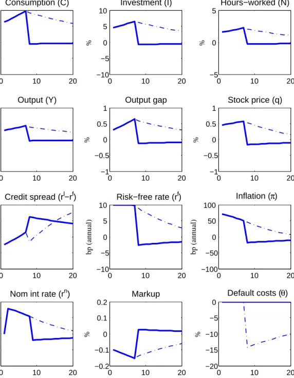
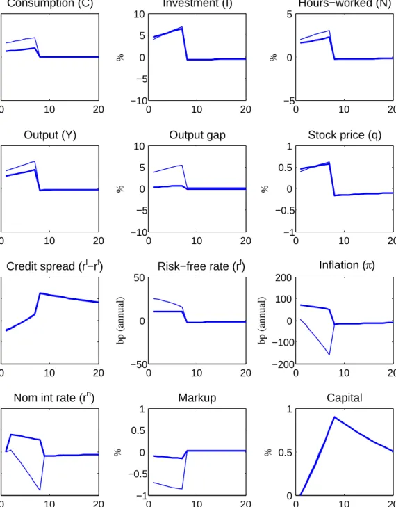
4.1.2 Model simulations of TFP news
The present model provides a nice illustration of the above discussion. Figure 3 shows the response of the model economy to news that TFP will rise by 1% in period 8. The broken line shows the path of the model economy when in period 8 TFP rises as expected, and the solid line shows the path of the model economy when in period 8 TFP fails to change as expected, remaining at steady state.
Note that the broken and solid line follow the same trajectory in the pre-shock phase since the dynamics during this phase are driven purely by the change in expectations. In response to the news shock, stock prices rise immediately and credit-spreads fall, and consumption, investment and hours-worked all rise. On the nominal side, both inflation and the nominal interest rate fall during the pre-shock phase.
The critical elements for understanding why this sticky price economy booms in re-sponse to news whereas the underlying flexible price economy contracts are the interaction of the inflation-targeting monetary policy rule with the financial accelerator under sticky prices. Note that in period 8 when the TFP shock hits, the demand for investment rises due to the impact of the shock on the marginal product of capital, and the impact of the shock drives down marginal costs. We can see this in the figure when in period 8 when the TFP shock hits, the broken line for the markup associated with the realization of the rise in TFP rises, meaning that marginal costs fall when the TFP shock hits. In response to the expected fall in future marginal costs, we expected price-setters in period 8 to
0 10 20 −2 0 2 4 Consumption (C) % 0 10 20 −5 0 5 10 Investment (I) % 0 10 20 −2 0 2 4 Hours−worked (N) % 0 10 20 −2 0 2 4 Output (Y) % 0 10 20 −5 0 5 10 Output gap % 0 10 20 −0.5 0 0.5 1 Stock price (q) % 0 10 20 −10 0 10 20 Credit spread (rl−rf) % 0 10 20 −50 0 50 Risk−free rate (rf) bp (annual) 0 10 20 −200 −100 0 100 Inflation (π) bp (annual) 0 10 20 −400 −200 0 200
Nom int rate (rn)
bp (annual) 0 10 20 −1 −0.5 0 0.5 Markup % 0 10 20 0 0.5 1 TFP (z) %
Figure 3: Expected rise in TFP under sticky prices. Response to news about 1% increase in TFP in period 8: TFP realized in period 8 (dashed line); TFP not realized in period 8 (solid line).
of period 8, faced with deflation, the inflation-targeting central bank lowers the policy rate, putting downward pressure on the risk-free rate and enhancing the overall boom. In the presence of adjustment costs, asset prices then rise in period 8 also as a result of the high investment.
How does this translate into a boom in period 1? From the perspective of period 1, asset prices rise today based on the expectation of the rise in asset prices in period 8. This sets off a chain of events that loosens credit conditions in period 1 since the rise in asset prices increases net worth of entrepreneurs, drives down contractual credit spreads, increasing the level of leverage consistent with the contract and as a result increasing the demand for new capital in the initial period. Under sticky prices, firms unable to change prices in period 1 meet this increase in demand by increasing production and decreasing the average markup. While the marginal costs fall in period 8 during the shock phase, it is clear form the figure that they rise during the demand-like pre-shock phase. Nevertheless the contribution of the persistent rise in marginal costs in the shock phase dominates and inflations falls initially as forward-looking price setters in period 1 lower prices. As a result, the central bank keeps the policy rate low during the initlal boom, further enhancing the boom. These effects combined with the wealth effect of the rise in future TFP on consumption allows a co-moving boom in response to news about a rise in future TFP. Note that the adjustment costs on capital here are a critical element; in their absence, there is no increase in assets prices to set off the financial accelerator effect, and no initial boom. The role of the inflation-targeting central bank is also critical in lowering the risk-free rate when the shock hits in period 8 to catalyze the boom8. This
mechanism through which an expected change in fundamentals in the future impacts credit conditions today is reminiscent of other models in the literature such as Jermann and Quadrini (2007), Walentin (2009) and Gortz and Tsoukalas (2012).
One thing to be clear about in this figure is that in response to news about TFP, the boom is completely inefficient, and entirely an artifact of the interaction of the sticky
8It is not necessary however that the central bank lower the policy rate in period 1 to achieve a boom
price aspects of the model with the financial accelerator framework and monetary policy rule. This is not necessarily a feature of the booms in the other models mentioned in the literature above. For example, in the model of Christiano et al. (2008), the efficient response of the flexible price RBC model underlying the NK model is for the primary aggregate quantities to boom in response to an expected rise in future TFP. In that model, adding sticky prices amplifies the boom in an inefficient matter through the the frictions of sticky prices, and adding sticky wages amplifies the boom considerably through inefficiencies in the labour market. In contrast, the response of the underlying flexible price model in this model economy to a rise in expected future TFP is much like that of the standard RBC model: consumption rises, yet investment, hours-worked and output fall. Yet adding sticky prices and an inflation targeting monetary policy rule reverses the direction of investment and hours, producing a boom in all primary quantities in response to news about TFP9.
Now focusing on the case of unfulfilled expectations, the path of the solid line depicts the case where in period 8 the agents find out that TFP does not rise as expected. Forward-looking firms able to adjust prices now face a lower path of expected future marginal costs higher than previously expected under expectations of the TFP shock, which all else equal results in an immediate upward revision of expected future marginal costs, and thus an upward revision in inflation expectations. Note in the figure that while in period 8 there is a sharp rise in inflation, it is still below steady state. Faced with an overaccumulation of capital, the demand for new capital falls, resulting in a textbook negative demand shock whereby firms unable to reduces prices lower production, raising markups. As such, despite the upward revision of marginal costs due the absence of any increase in TFP, marginal costs and thus inflation still remain below steady state during the bust. Faced with low inflation, the inflation-targeting central bank as a result lowers the policy rate. Thus overall under the TFP-driven boom bust, we see below steady state inflation during both the pre-shock boom phase as well as the unfulfilled bust phase.
9One could readily add additional structural features to the present model such that under flexible
prices all primary quantities boom as in Christiano et al. (2008), but doing so would unnecessarily complicate the model and obfuscate some of the mechanisms that I will describe later.
4.2
Fluctuations in default costs
θ
I now consider the response of the model economy to variation in the cost of default θ. To clearly understand the impact of changes inθ, I first consider a contemporaneous and expected change in θ in the model economy with flexible prices.
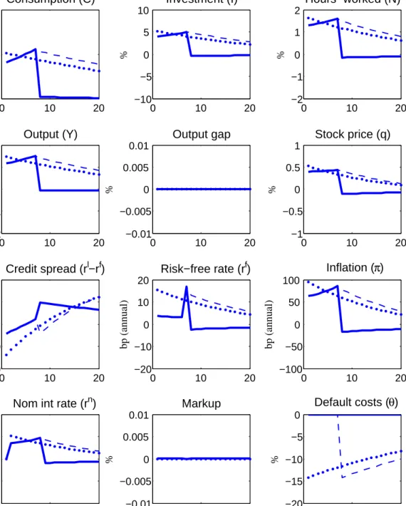
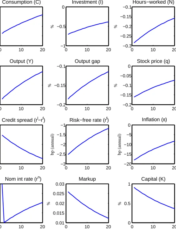
4.2.1 A contemporaneous and expected fall in θ under flexible prices
Figure 4 shows the response of the flexible priced version of the model economy to a surprise contemporaneous 14.2% fall in θ, and as well the realized and unrealized cases of news about an expected 14.2% fall in θ in period 8. Since with flexible prices the response of the real side of the economy is essentially the same as in the real economy of Gunn and Johri (2013a), I discuss them only briefly.
Beginning with the contemporaneous shock, note that the surprise fall in θ causes an immediate boom in consumption, investment, hours-worked and output, along with a rise in asset prices and fall in the credit spread. While the initial fall in θ in period 1 has a small impact effect through the bank’s zero profit condition that increases the entrepreneurs net-worth slightly in period 1, the most significant effect occurs through the impact of the persistent fall inθ in the financial contract: each entrepreneur’s choice of capital in period 1 depends on state state of the economy in period t+ 1. Since the shock toθt is persistent,θt+1 will also be low, shifting out the menu of financial contracts
available such that the entrepreneurs can increase their leverage for a given external finance premium, meaning that entrepreneurs can choose a higher level of new capital and still satisfy the contract terms. Thus the fall in θ ultimately leads to an increase in demand for investment.
How does this fall in the demand for new capital transmit into the overall economy? Since the shock to θ has no direct impact on the production function and the shock as a result does nothing to loosen the economy’s resource constraint, in this flexible price economy the marginal utility of consumptionλt and real interest rate must rise such that
0 10 20 0 0.5 1 Consumption (C) % 0 10 20 −10 −5 0 5 10 Investment (I) % 0 10 20 −2 −1 0 1 2 Hours−worked (N) % 0 10 20 −2 −1 0 1 2 Output (Y) % 0 10 20 −0.01 −0.005 0 0.005 0.01 Output gap % 0 10 20 −1 −0.5 0 0.5 1 Stock price (q) % 0 10 20 −20 −10 0 10 20 Credit spread (rl−rf) % 0 10 20 −20 −10 0 10 20 Risk−free rate (rf) bp (annual) 0 10 20 −100 −50 0 50 100 Inflation (π) bp (annual) 0 10 20 −200 −100 0 100 200
Nom int rate (rn)
bp (annual) 0 10 20 −0.01 −0.005 0 0.005 0.01 Markup % 0 10 20 −20 −15 −10 −5 0 Default costs (θ) %
Figure 4: Contemporaneous versus expected fall in default costs θ under flex-ible prices. Response to contemporaneous 14.2% fall in θ (dotted line); Response to news about 14.2% fall in period 8 -θ realized in period 8 (broken line), θ not realized in period 8 (solid line).
by the household. Indeed under separable preferences (not shown), consumption falls while investment, hours and output rise. Consumption is not fully crowded out however since the rise inλtmeans that labour supply shifts out as the household substitutes leisure
form the present into the future, driving up equilibrium hours-worked, capacity utilization and therefore output in equilibrium. Only under the non-separable preferences does consumption rise also since the marginal utilization of consumption is increasing in hours-worked, allowing a rise in consumption to be consistent with a high marginal utilization of consumption. Moreover the rise in consumption alongside the rise in investment is made possible by the additional output induced by the outward shift in labour supply and resulting rise in equilibrium hours-worked.
Now turning to news about future changes in θ, the thick line in the figure which shows the response of the model economy to news that θ will rise in period 8. The key to understanding this effect is to consider that from the perspective of period 1 when the news is received, agents now expect that in period 8 the impact effect of the economy in period 8 of the shock toθ in that period 8 will be as described for the contemporaneous shock above in period 1. To be specific, in period 1, agents expect that in period 7 (when entrepreneurs first choose new capital under a contract that reflects the expected fall inθ the following period) there will be an increase in demand for new capital, along with a high marginal utility of consumption and high risk-free rate in period 7. The forward-looking effect of the household’s Euler equation then implies that the future rise in the marginal utility of consumption induces a rise in the marginal utilization of consumption in the present, unleashing the intertemporal substitution effects in the present similar to those in the contemporaneous case, whereby the outward shift in labour supply from the rise inλ droves up equilibrium hours-worked, utilization and output, while still permitting a rise in consumption in the present.
Note that the effect here lies in direct contrast to the case of news about a rise in TFP. When TFP hits in the future, its effect of loosening the economy’s resource constraint results in a low marginal utilization of consumption in the future, resulting in a lower marginal utilization of consumption in the present also, and thus an intertemoral
wealth effect that under flexible prices induces the household to raise consumption and lower hours-worked in the present, resulting in a contraction. The literature as a result has spent considerable effort introducing structural mechanisms to break or weaken this wealth effect on leisure. The case of news about the fall in θ does not suffer this same challenge, since the effect of a fall in θ in the future is to drive the marginal utilization of consumption upwards rather than downwards. As a result, in contrast to TFP boom-busts, for the credit boom-bust under flexible prices the economy exhibits procyclical co-movement with relatively few structural modifications relative to a standard DSGE model.
Now focusing on the case of unfulfilled expectations, the path of the solid line depicts the case where in period 8 the agents learn that default costs θ will not fall as they had previously expected. Entrepreneurs now suddenly find themselves with too much capital given the state of the world, and as a result the demand for new capital plummets. This drop in the demand for capital drives down the risk-free rate, setting in a chain of events which now contracts labour supply and reduces capicity utilization, reducing the equilibrium level of output and investment and consumption.
Turning to the nominal side of the model economy for both the surprise and antici-pated cases in the figure, note that under flexible prices, the nominal side of the linearized model economy effectively consists of a Fisher equation and the simple monetary rule, given respectively as
rft =rtn−Etπt+1 (35)
rnt =φππt, (36)
where the interest rates and inflation are expressed as (absolute) deviations from steady state. These two equations can be combined to form a single expectational difference equation inπtwith the real ratertf as a forcing variable, being determined completely by
of expected future real rates πt= ∞ X k=0 (1/φπ)krtf+k. (37)
Note that the parameter φπ represents the stance of monetary policy in determining the
price level here, such that looser inflation targeting represented by a lower φπ results in
a higher rate of price growth.
Figure 4 shows that inflation rises immediately to its peak in period 1 under the surprise shock, whereas under the anticipated shock, inflation rises initially and then continues to climb until reaching its peak in period 7. Consistent with the above discus-sion, the path of inflation in both of these cases is driven by the realized and expected path of the real-rate: in the former, the real rate rises to its peak in period 1, whereas in the latter the real rate rises and then continues to climb to its peak in period 7. Given the monetary rule that simply leans against inflation, the path of the nominal policy rate in both these cases thus follows that of the respective inflation rates. Under the anticipated case, if in period 8 default costs θ turn out not too fall, note that the sudden drop in the current and expectured future real rates now drives inflation below steady state.
Note that in both of the scenarios, the rise in inflation is low: less than 80 basis points on an annualized basis relative to an approximately 1.5% expansion of output. Recent literature such as Beaudry and Portier (2013b) has suggested that New Keynesian models might suggest a volatility of inflation relative to the output gap that is larger that seen in the data. With regard to this critique, I make two points relative to the results of this model thus far. First, in sticky-price frameworks, the literature such as Christiano et al. (2005) has discussed the role of capacity utilization on keeping a lid on inflation in response to demand-shocks through its impact in limiting the rise in marginal costs. Even here under flexible prices capacity utilization plays an important role in maintaining low inflation over the real boom through its effect of limiting the rise of the risk-free rate. Indeed, removing the effect of utilization in the above exercise (not shown) reduces the size of the boom in output by more than half, yet nearly doubles the rise in the risk-free rate and the inflation rate.
Secondly, on a more subtle note, and a point that is particularly important to assessing the nominal impact of news shocks, the observations of Beaudry and Portier (2013b) pertain to the relation between inflation and the output gap. As Uribe (2013) discusses, the output gap (or the natural level of ouput) is a model-specific notion. Using an empirical measure of the output gap such as the deviation of output from a smooth trend or HP-filtered variations as in Beaudry and Portier (2013b) may be inconsistent with a given model if the model implies variation in the flexible price level of output in response to a given shock10. As we will see when we add sticky prices, only part of the credit boom in this model is made up of movement in the output gap; a large fraction of the boom still consists of the rise in the natural level of output to news driven by the rise in the real rate of return. Thus even if a given New Keynesian model such as this one implies a high volatility of inflation relative to the output gap per-se in response to the demand-driven boom phase of a news shock, this does not necessarily mean that it implies a high volatility of inflation to output: any inflationary movements driven by a rise in the output gap will contribute only partly to the overall relation between inflation and output overall, the other contribution between the rise in the flexible price level of output in response to the same shock. This is particularly important when empirically-derived estimates of the output gap are not model specific, but rather, use a measure such as deviation of output from a smooth trend. Taking the output of the above exercise under flexible prices as artificial data, using such a measure of the output gap would then imply an empirical relation between inflation and the output gap, even though the model specific output gap is zero, as shown in the figure.
As this discussion highlights, it is important to understand the relative contribution of the flexible and non-flexible components of output variation of a news-driven boom in a given model economy. Models that rely more in inefficiencies of nominal rigidities and
10I stress the may in this statement. For example, Beaudry and Portier (2013b) motivate their
approach by considering the response of a labour-only NK model to news about future TFP. In that particular example, in the absence of capital, under flexible prices output does not fluctuate at all in response to news about future TFP since once can show that consumption is proportional to current TFP, which doesn’t change until the future. As a result, any boom associated with introducing sticky prices in that example is completely a result of movements in the output gap, and thus consistent with BP’s empirical measure of the output gap as the HP-filtered variation in output.
a suboptimal rule to generate a boom in response to a news shock (as in the early case of TFP-news in this paper) will have a large contribution of the output gap to the overall boom in output, and thus imply a structural relation between inflation and output that is influenced more by the impact of the countercyclical markups than in an alternative model where the underlying flexible economy booms in response to the news shock.
4.2.2 An expected fall in θ under sticky prices
What is clear from above discussion is that under flexible prices, the rise in demand for new capital is dependent on intertemporal substitution to induce the initial boom, and the intertemporal substitution in turn drives the behaviour of the nominal side of the economy through the dependence of the inflation rate on current and expected real rates. Adding nominal rigidities breaks this simple dependency