NBER WORKING PAPER SERIES
OPTIMAL INFLATION TARGETING RULES Marc P. Giannoni
Michael Woodford Working Paper9939
http://www.nber.org/papers/w9939
NATIONAL BUREAU OF ECONOMIC RESEARCH 1050 Massachusetts Avenue
Cambridge, MA 02138 August 2003
This is a revised draft of a paper prepared for the NBER conference on Inflation Targeting, Miami, Florida, January 23-25, 2003. We would like to thank Jean Boivin, Rick Mishkin, Ed Nelson, and Lars Svensson for helpful discussions, Brad Strum for research assistance, and the National Science Foundation for research support through a grant to the NBER. The views expressed herein are those of the authors and not necessarily those of the National Bureau of Economic Research.
©2003 by Marc P. Giannoni and Michael Woodford. All rights reserved. Short sections of text, not to exceed two paragraphs, may be quoted without explicit permission provided that full credit, including © notice, is given to the source.
Optimal Inflation Targeting Rules
Marc P. Giannoni and Michael Woodford NBER Working Paper No. 9939
August 2003 JEL No. E52, E61
ABSTRACT
This paper characterizes optimal monetary policy for a range of alternative economic models in terms of a flexible inflation targeting rule, with a target criterion that depends on the model specification. It shows which forecast horizons should matter, and which variables besides inflation should be taken into account, for each specification.
The likely quantitative significance of the various factors considered in the general discussion is then assessed by estimating a small, structural model of the U.S. monetary transmission mechanism with explicit optimizing foundations. An optimal policy rule is computed for the estimated model, and shown to correspond to a multi-stage inflation-forecast targeting procedure. The degree to which actual U.S. policy over the past two decades has conformed to the optimal target criteria is then considered.
Marc P. Giannoni Michael Woodford
Graduate School of Business Department of Economics
Columbia University Princeton University
3022 Broadway Princeton, NJ 08544
New York, NY 10027 and NBER
An increasingly popular approach to the conduct of monetary policy, since the early 1990s, has been inflation-forecast targeting. Under this general approach, a central bank is committed to adjust short-term nominal interest rates periodically so as to ensure that its projection for the economy’s evolution satisfies an explicit target criterion — for example, in the case of the Bank of England, the requirement that the RPIX inflation rate be projected to equal 2.5 percent at a horizon two years in the future (Vickers, 1998). Such a commitment can overcome the inflationary bias that is likely to follow from discretionary policy guided solely by a concern for social welfare, and can also help to stabilize medium-term inflation expectations around a level that reduces the output cost to the economy of maintaining low inflation.
Another benefit that is claimed for such an approach (e.g., King, 1997; Bernanke et al., 1999)— and an important advantage, at least in principle, of inflation targeting over other policy rules, such as a k-percent rule for monetary growth, that should also achieve a low average rate of inflation — is the possibility of combining reasonable stability of the inflation rate (especially over the medium to long term) with optimal short-run responses to real disturbances of various sorts. Hence Svensson (1999) argues for the desirability of “flexible” inflation targeting, by which it is meant1that the target criterion involves not only the projected path of the inflation rate, but one or more other variables, such as a measure of the output gap, as well.
We here consider the question of what sort of additional variables ought to matter — and with what weights, and what dynamic structure — in a target criterion that is intended to implement optimal policy. We wish to use economic theory to address questions such as which measure of inflation is most appropriately targeted (an index of goods prices only, or wage inflation as well?), which sort of output gap, if any, should justify short-run departures of projected inflation from the long-run target rate (a departure of real GDP from a smooth
1Svensson discusses two alternative specifications of an inflation-targeting policy rule, one of which (a
“general targeting rule”) involves specification of a loss function that the central bank should use to evaluate alternative paths for the economy, and the other of which (a “specific targeting rule”) involves specification of a target criterion. We are here concerned solely with policy prescriptions of the latter sort. On the implementation of optimal policy through a “general targeting rule,” see Svensson and Woodford (2003).
trend path, or from a “natural rate” that varies in response to a variety of disturbances?), and how large a modification of the acceptable inflation projection should result from a given size of projected output gap. We also consider how far in the future the inflation and output projections should extend upon which the current interest-rate decision is based, and the degree to which an optimal target criterion should behistory-dependent, i.e., should depend on recent conditions, and not simply on the projected paths of inflation and other target variables from now on.
In a recent paper (Giannoni and Woodford, 2002a), we expound a general approach to the design of an optimal target criterion. We show, for a fairly general class of linear-quadratic policy problems, how it is possible to choose a target criterion that will satisfy several desiderata. First, the target criterion has the property that insofar as the central bank is expected to ensure that it holds at all times, this expectation will imply the existence of a determinate rational-expectations equilibrium. Second, that equilibrium will be optimal, from the point of view of a specified quadratic loss function, among all possible rational-expectations equilibria, given one’s model of the monetary transmission mechanism.2 Thus the policy rule implements the optimal state-contingent evolution of the economy, in the sense of giving it a reason to occur if the private sector is convinced of the central bank’s commitment to the rule and fully understands its implications.
Third, the rule is robustly optimal, in the sense that the same target criterion brings about an optimal state-contingent evolution of the economy regardless of the assumed statistical properties of the exogenous disturbances, despite the fact that the target criterion makes no explicit reference to the particular types of disturbances that may occur (except insofar as these may be involved in the definition of the target variables — the variables appearing
2Technically, the state-contingent evolution that is implemented by commitment to the policy rule is
optimal from a “timeless perspective” of the kind proposed in Woodford (1999b), which means that it would have been chosen as part of an optimal commitment at a date sufficiently far in the past for the policymaker to fully internalize the implications of the anticipation of the specified policy actions, as well as their effects at the time that they are taken. This modification of the concept of optimality typically used in Ramsey-style analyses of optimal policy commitments allows a time-invariant policy rule to be judged optimal, and eliminates the time inconsistency of optimal policy. See Giannoni and Woodford (2002a) and Svensson and Woodford (2003) for further discussion.
in the loss function which defines the stabilization objectives). This robustness greatly increases the practical interest in the computation of a target criterion that is intended to implement optimal state-contingent responses to disturbances; for actual economies are affected by an innumerable variety of types of disturbances, and central banks always have a great deal of specific information about the ones that have most recently occurred. The demand that the target criterion be robustly optimal also allows us to obtain much sharper conclusions as to the form of an optimal target criterion. For while there would be a very large number of alternative relations among the paths of inflation and other variables that are equally consistent with the optimal state-contingent evolution in the case of a particular type of assumed disturbances, only relations of a very special sort continue to describe the optimal state-contingent evolution even if one changes the assumed character of the exogenous disturbances affecting the economy.
Our general characterization in Giannoni and Woodford (2002a) is in terms of a fairly abstract notation, involving eigenvectors and matrix lag polynomials. Here we offer examples of the specific character of the optimally flexible inflation targets that can be derived using that theory. Our results are of two sorts. First, we illustrate the implications of the theory in the context of a series of simple models that incorporate important features of realistic models of the monetary transmission mechanism. Such features include wage and price stickiness, inflation inertia, habit persistence, and predeterminedness of pricing and spending decisions. In the models considered, there is a tension between two or more of the central bank’s stabilization objectives, that cannot simultaneously be achieved in full; in the simplest case, this is a tension between inflation and output-gap stabilization, but we also consider models in which it is reasonable to seek to stabilize interest rates or wage inflation as well. These results in the context of very simple models are intended to give insight into the way in which the character of the optimal target criterion should depend on one’s model of the economy, and should be of interest even to readers who are not persuaded of the empirical realism of our estimated model.
transmis-sion mechanism, the numerical parameters of which are fit to VAR estimates of the impulse responses of several aggregate variables to identified monetary policy shocks. While the model remains an extremely simple one, this exercise makes an attempt to judge the likely quantitative significance of the types of effects that have previously been discussed in more general terms. It also offers a tentative evaluation of the extent to which U.S. policy over the past two decades has differed from what an optimal inflation-targeting regime would have called for.
1
Model Specification and Optimal Targets
Here we offer a few simple examples of the way in which the optimal target criterion will depend on the details of one’s model of the monetary transmission mechanism. (The optimal target criterion also depends, of course, on one’s assumed stabilization objectives. But here we shall take the view that the appropriate stabilization objectives follow from ones assumptions about the way in which policy affects the economy, though the welfare-theoretic stabilization objectives implied by our various simple models are here simply asserted rather than derived.) The examples that we select illustrate the consequences of features that are often present in quantitative optimizing models of the monetary transmission mechanism. They are also features of the small quantitative model presented in section 2; hence our analytical results in this section are intended to provide intuition for the numerical results presented for the empirical model in section 3.
The analysis of Giannoni and Woodford (2002a) derives a robustly optimal target crite-rion from the first-order conditions that characterize the optimal state-contingent evolution of the economy. Here we illustrate this method by directly applying it to our simple examples, without any need to recapitulate the general theory.
1.1
An Inflation-Output Stabilization Tradeoff
We first consider the central issue addressed in previous literature on flexible inflation target-ing, which is the extent to which a departure from complete (and immediate) stabilization of
inflation is justifiable in the case of real disturbances that prevent joint stabilization of both inflation and the (welfare-relevant) output gap.3 We illustrate how this question would be answered in the case of a simple optimizing model of the monetary transmission mechanism that allows for the existence of such “cost-push shocks” (to use the language of Clarida et al., 1999).
As is well known, a discrete-time version of the optimizing model of staggered price-setting proposed by Calvo (1983) results in a log-linear aggregate supply relation of the form
πt=κxt+βEtπt+1+ut, (1.1)
sometimes called the “New Keynesian Phillips curve” (after Roberts, 1995).4 Hereπ
tdenotes the inflation rate (rate of change of a general index of goods prices), xt the output gap (the deviation of log real GDP from a time-varying “natural rate”, defined so that stabilization of the output gap is part of the welfare-theoretic stabilization objective5), and the disturbance termutis a “cost-push shock”, collecting all of the exogenous shifts in the equilibrium relation between inflation and output that do not correspond to shifts in the welfare-relevant “natural rate” of output. In addition, 0< β <1 is the discount factor of the representative household, and κ > 0 is a function of a number of features of the underlying structure, including both the average frequency of price adjustment and the degree to which Ball-Romer (1990) “real rigidities” are important.
We shall assume that the objective of monetary policy is to minimize the expected value
3Possible sources of disturbances of this sort are discussed in Giannoni (2000), Steinsson (2002), and
Woodford (2003, chap. 6).
4See Woodford (2003, chap. 3) for a derivation in the context of an explicit intertemporal general
equi-librium model of the transmission mechanism. Equation (1.1) represents merely a log-linear approximation to the exact equilibrium relation between inflation and output implied by this pricing model; however, un-der circumstances discussed in Woodford (2003, chap. 6), such an approximation suffices for a log-linear approximate characterization of the optimal responses of inflation and output to small enough disturbances. Similar remarks apply to the other log-linear models presented below.
5See Woodford (2003, chaps. 3 and 6) for discussion of how this variable responds to a variety of types of
real disturbances. Under conditions discussed in chapter 6, the “natural rate” referred to here corresponds to the equilibrium level of output in the case that all wages and prices were completely flexible. However, our results in this section apply to a broader class of model specifications, under an appropriate definition of the “output gap”.
of a loss function of the form W =E0 (∞ X t=0 βtLt ) , (1.2)
where the discount factor β is the same as in (1.1), and the loss each period is given by
Lt=π2t +λ(xt−x∗)2, (1.3)
for a certain relative weight λ > 0 and optimal level of the output gap x∗ > 0. Under
the same microfoundations as justify the structural relation (1.1), one can show (Woodford, 2003, chap. 6) that a quadratic approximation to the expected utility of the representative household is a decreasing function of (1.2), with
λ =κ/θ (1.4)
(where θ > 1 is the elasticity of substitution between alternative differentiated goods) and
x∗ a function of both the degree of market power and the size of tax distortions. However,
we here offer an analysis of the optimal target criterion in the case of any loss function of the form (1.3), regardless of whether the weights and target values are the ones that can be justified on welfare-theoretic grounds or not. (In fact, a quadratic loss function of this form is frequently assumed in the literature on monetary policy evaluation, and is often supposed to represent the primary stabilization objectives of actual inflation-targeting central banks in positive characterizations of the consequences of inflation targeting.)
The presence of disturbances of the kind represented by ut in (1.1) creates a tension between the two stabilization goals reflected in (1.3) of inflation stabilization on the one hand and output-gap stabilization (around the value x∗) on the other; under an optimal policy,
the paths of both variables will be affected by cost-push shocks. The optimal responses can be found by computing the state-contingent paths{πt, xt} that minimize (1.2) with loss function (1.3) subject to the sequence of constraints (1.1).6 The Lagrangian for this problem,
6Note that the aggregate-demand side of the model does not matter, as long as a nominal interest-rate
path exists that is consistent with any inflation and output paths that may be selected. This is true if, for example, the relation between interest rates and private expenditure is of the form (1.15) assumed below, and the required path of nominal interest rates is always non-negative. We assume here that the non-negativity constraint never binds, which will be true, under the assumptions of the model, in the case of any small enough real disturbances{ut, rnt}.
looking forward from any datet0, is of the form Lt0 =Et0 ∞ X t=t0 βt−t0 ½1 2[π 2 t +λx(xt−x∗)2] +ϕt[πt−κxt−βπt+1] ¾ , (1.5)
where ϕt is a Lagrange multiplier associated with constraint (1.1) on the possible inflation-output pairs in period t. In writing the constraint term associated with the period t AS relation, it does not matter that we substitute πt+1 forEtπt+1; for it is only the conditional expectation of the term at datet0 that matters in (1.5), and the law of iterated expectations implies that
Et0[ϕtEtπt+1] = Et0[Et(ϕtπt+1)] =Et0[ϕtπt+1] for any t≥t0.
Differentiating (1.5) with respect to the levels of inflation and output each period, we obtain a pair of first-order conditions
πt+ϕt−ϕt−1 = 0, (1.6)
λ(xt−x∗)−κϕt= 0, (1.7)
for each period t ≥ t0. These conditions, together with the structural relation (1.1), have a unique non-explosive solution7 for the inflation rate, the output gap, and the Lagrange multiplier (a unique solution in which the paths of these variables are bounded if the shocks
ut are bounded), and this solution (which therefore satisfies the transversality condition) indicates the optimal state-contingent evolution of inflation and output.
As an example, Figure 1, plots the impulse responses to a positive cost-push shock, in the simple case that the cost-push shock is purely transitory, and unforecastable before the period in which it occurs (so thatEtut+j = 0 for all j ≥1). Here the assumed values ofβ, κ,
7Obtaining a unique solution requires the specification of an initial value for the Lagrange multiplierϕ t0−1. See Woodford (2003, chap. 7) for the discussion of alternative possible choices of this initial condition and their significance. Here we note simply that regardless of the value chosen forϕt0−1,the optimal responses to cost-push shocks in periodt0 and later are the same.
0 2 4 6 8 10 12 −2 0 2 4 inflation 0 2 4 6 8 10 12 −5 0 5 output 0 2 4 6 8 10 12 0 0.5 1 1.5 2 price level = optimal = non−inertial
Figure 1: Optimal responses to a positive cost-push shock under commitment, in the case of Calvo pricing.
and λ are those given in Table 1,8 and the shock in period zero is of sizeu
0 = 1; the periods represent quarters, and the inflation rate is plotted as an annualized rate, meaning that what is plotted is actually 4πt. As one might expect, in an optimal equilibrium inflation is allowed to increase somewhat in response to a cost-push shock, so that the output gap need not fall as much as would be required to prevent any increase in the inflation rate. Perhaps less intuitively, the figure also shows that under an optimal commitment, monetary policy remains tight even after the disturbance has dissipated, so that the output gap returns to
8These parameter values are based on the estimates of Rotemberg and Woodford (1997) for a slightly
more complex variant of the model used here and in section 1.3. The coefficientλhere corresponds toλx in
the table. Note also that the value of .003 for that coefficient refers to a loss function in whichπtrepresents
thequarterly change in the log price level. If we write the loss function in terms of an annualized inflation rate, 4πt,as is conventional in numerical work, then the relative weight on the output-gap stabilization term
would actually be 16λx,or about .048. Of course, this is still quite low compared the relative weights often
assumed in thead hoc stabilization objectives used in the literature on the evaluation of monetary policy rules.
Table 1: Calibrated parameter values for the examples in section 1. Structural parameters β 0.99 κ .024 θ−1 0.13 σ−1 0.16 Shock processes ρu 0 ρr 0.35 Loss function λx .003 λi .236
zero only much more gradually. As a result of this, while inflation overshoots its long-run target value at the time of the shock, it is held below its long-run target value for a time following the shock, so that the unexpected increase in prices is subsequently undone. In fact, as the bottom panel of the figure shows, under an optimal commitment, the price level eventually returns to exactly the same path that it would have been expected to follow if the shock had not occurred.
This simple example illustrates a very general feature of optimal policy once one takes account of forward-looking private-sector behavior: optimal policy is almost always history-dependent. That is, it depends on the economy’s recent history and not simply on the set of possible state-contingent paths for the target variables (here, inflation and the output gap) that are possible from now on. (In the example shown in the figure, the set of pos-sible rational-expectations equilibrium paths for inflation and output from period t onward depends only on the value of ut; but under an optimal policy, the actually realized inflation rate and output gap depend on past disturbances as well.) This is because a commitment to respond later to past conditions can shift expectations at the earlier date in a way that helps to achieve the central bank’s stabilization objectives. In the present example, if price-setters are forward-looking, the anticipation that a current increase in the general price level will
predictably be “undone” soon gives suppliers a reason not to increase their own prices cur-rently as much as they otherwise would. This leads to smaller equilibrium deviations from the long-run inflation target at the time of the cost-push shock, without requiring such a large change in the output gap as would be required to stabilize inflation to the same degree without a change in expectations regarding future inflation. (The impulse responses under the best possible equilibrium that does not involve history-dependence are shown by the dashed lines in the figure.9 Note that a larger initial output contraction is required, even though both the initial price increase and the long-run price increase caused by the shock are greater.)
It follows that no purely forward-looking target criterion — one that involves only the projected paths of the target variables from the present time onward, like the criterion that is officially used by the Bank of England — can possibly determine an equilibrium with the optimal responses to disturbances. Instead, a history-dependent target criterion is necessary, as stressed by Svensson and Woodford (2003).
A target criterion that works is easily derived from the first-order conditions (1.6) – (1.7). Eliminating the Lagrange multiplier, one is left with a linear relation
πt+φ(xt−xt−1) = 0, (1.8)
with a coefficientφ=λ/κ >0,that the state-contingent evolution of inflation and the output gap must satisfy. Note that this relation must hold in an optimal equilibrium regardless of the assumed statistical properties of the disturbances. One can also show that a commitment to ensure that (1.8) holds each period from some date t0 onward implies the existence of a determinate rational-expectations equilibrium,10 given any initial output gap x
t0−1. In this
equilibrium, inflation and output evolve according to the optimal state-contingent evolution
9See Woodford (2003, chap. 7) for derivation of this “optimal non-inertial plan.” In the example shown in
Figure 1, this optimal non-inertial policy corresponds to the Markov equilibrium resulting from discretionary optimization by the central bank. That equivalence would not obtain, however, in the case of serially correlated disturbances.
10The characteristic equation that determines whether the system of equations consisting of (1.1) and (1.8)
has a unique non-explosive solution is the same as for the system of equations solved above for the optimal state-contingent evolution.
characterized above.
This is the optimal target criterion that we are looking for: it indicates that deviations of the projected inflation rate πt from the long-run inflation target (here equal to zero) should be accepted that are proportional to the degree to which the output gap is projected to decline over the same period that prices are projected to rise. Note that this criterion is history-dependent, because the acceptability of a given projection (πt, xt) depends on the recent past level of the output gap; it is this feature of the criterion that will result in the output gap’s returning only gradually to its normal level following a transitory cost-push shock, as shown in Figure 1.
How much of a projected change in the output gap is needed to justify a given degree of departure from the long-run inflation target? If λ is assigned the value that it takes in the welfare-theoretic loss function, then φ =θ−1, where θ is the elasticity of demand faced by the typical firm. The calibrated value for this parameter given in Table 1 (based on the estimates of Rotemberg and Woodford, 1997) implies that φ=.13. If we express the target criterion in terms of the annualized inflation rate (4πt) rather than the quarterly rate of price change, the relative weight on the projected quarterly change in the output gap will instead be 4φ, or about 0.51. Hence a projection of a decline in real GDP of two percentage points relative to the natural rate of output over the coming quarter would justify an increase in the projected (annualized) rate of inflation of slightly more than one percentage point.
1.2
Inflation Inertia
A feature of the “New Keynesian” aggregate-supply relation (1.1) that has come in for substantial criticism in the empirical literature is the fact that past inflation rates play no role in the determination of current equilibrium inflation. Instead, empirical models of the kind used in central banks for policy evaluation often imply that the path of the output gap required in order to achieve a particular path for the inflation rate from now onward depends on what rate of inflation has already been recently experienced; and this aspect of one’s model is of obvious importance for the question of how rapidly one should expect
that it is optimal to return inflation to its normal level, or even to “undo” past unexpected price-level increases, following a cost-push shock.
A simple way of incorporating inflation inertia of the kind that central-bank models often assume into an optimizing model of pricing behavior is to assume, as Christiano et al. (2001) propose, that individual prices are indexed to an aggregate price index during the intervals between re-optimizations of the individual prices, and that the aggregate price index becomes available for this purpose only with a one-period lag. When the Calvo model of staggered price-setting is modified in this way, the aggregate-supply relation (1.1) takes the more general form11
πt−γπt−1 =κxt+βEt[πt+1−γπt] +ut, (1.9) where the coefficient 0≤γ ≤1 indicates the degree of automatic indexation to the aggregate price index. In the limiting case of complete indexation (γ = 1), the case assumed by Christianoet al. and the case found to best fit US data in our own estimation results below, this relation is essentially identical to the aggregate-supply relation proposed by Fuhrer and Moore (1995), which has been widely used in empirical work.
The welfare-theoretic stabilization objective corresponding to this alternative structural model is of the form (1.2) with the period loss function (1.3) replaced by
Lt= (πt−γπt−1)2+λ(xt−x∗)2, (1.10) where λ >0 is again given by (1.4), and x∗ >0 is similarly the same function of underlying
microeconomic distortions as before.12 (The reason for the change is that with the automatic indexation, the degree to which the prices of firms that re-optimize their prices and those that do not are different depends on the degree to which the current overall inflation rate
πt differs from the rate at which the automatically adjusted prices are increasing,i.e., from
γπt−1.) If we consider the problem of minimizing (1.2) with loss function (1.10) subject to
11See Woodford (2003, chap. 3) for a derivation from explicit microeconomic foundations.
0 2 4 6 8 10 12 −2 0 2 4 inflation 0 2 4 6 8 10 12 −6 −4 −2 0 2 output 0 2 4 6 8 10 12 0 0.5 1 1.5 2 price level γ = 0 γ = 0.5 γ = 0.8 γ = 1.0
Figure 2: Optimal responses to a positive cost-push shock under commitment, for alternative degrees of inflation inertia.
the sequence of constraints (1.9), the problem has the same form as in the previous section, except with πt everywhere replaced by the quasi-differenced inflation rate
πqdt ≡πt−γπt−1. (1.11)
The solution is therefore also the same, with this substitution.
Figure 2 shows the impulse responses of inflation, the output gap, and the price level to the same kind of disturbance as in Figure 1, under optimal policy for economies with alter-native values of the indexation parameter γ. (The values assumed for β, κ, and λ are again as in Table 1.) Once again, under an optimal commitment, the initial unexpected increase in prices is eventually undone, as long as γ < 1; and this once again means that inflation eventually undershoots its long-run level for a time. However, for any large enough value of γ, inflation remains greater than its long-run level for a time even after the disturbance
has ceased, and only later undershoots its long-run level; and the larger is γ,the longer this period of above-average inflation persists. In the limiting case thatγ = 1,the undershooting never occurs; inflation is simply gradually brought back to the long-run target level.13 In this last case, a temporary disturbance causes a permanent change in the price level, even under optimal policy. However, the inflation rate is eventually restored to its previously anticipated long-run level under an optimal commitment, even though the rate of inflation (as opposed to the rate of acceleration of inflation) is not welfare-relevant in this model. (Note that the optimal responses shown in Figure 2 for the case γ = 1 correspond fairly well to the conventional wisdom of inflation-targeting central banks; but our theoretical analysis allows us to compute an optimal rate at which inflation should be projected to return to its long-run target value following a disturbance.)
As in the previous section, we can derive a target criterion that implements the optimal responses to disturbances regardless of the assumed statistical properties of the disturbances. This optimal target criterion is obtained by replacing πt in (1.8) byπqdt , yielding
πt−γπt−1+φ(xt−xt−1) = 0, (1.12)
where φ > 0 is the same function of model parameters as before. This indicates that the acceptable inflation projection for the current period should depend not only on the projected change in the output gap, but also (insofar as γ >0) on the recent past rate of inflation: a higher existing inflation rate justifies a higher projected near-term inflation rate, in the case of any given output-gap projection.
In the special case that γ = 1, the optimal target criterion adjusts the current inflation target one-for-one with increases in the existing rate of inflation — the target criterion actually involves only the rate of acceleration of inflation. But this does not mean that disturbances are allowed to permanently shift the inflation rate to a new level, as shown in Figure 2. In fact, in the case of full indexation, an alternative target criterion that also leads
13Note that the impulse response of inflation (forγ= 1) in panel 1 of Figure 2 is the same as the impulse
response of the price level (under optimal policy) in panel 3 of Figure 1. The scales are different because the inflation rate plotted is an annualized rate, 4πtrather thanπt.
to the optimal equilibrium responses to cost-push shocks is the simpler criterion
πt+φxt= ¯π, (1.13)
where againφ >0 is the same coefficient as in (1.12), and the value of the long-run inflation target ¯π is arbitrary (but not changing over time). Note that (1.12) is just a first-differenced form of (1.13), and a commitment to ensure that (1.12) holds in each period t ≥ t0 is equivalent to a commitment to ensure that (1.13) holds, for a particular choice of ¯π, namely ¯
π =πt0−1+φxt0−1.But the choice of ¯π has no effect on either the determinacy of equilibrium
or the equilibrium responses of inflation and output to real disturbances (only on the long-run average inflation rate), and so any target criterion of the form (1.13) implements the optimal responses to disturbances.14 Note that this optimal target criterion is similar in form to the kind that Svensson (1999) suggests as a description of the behavior of actual inflation-targeting central banks, except that the inflation and output-gap projections in (1.13) are not so far in the future (they refer only to the coming quarter) as in the procedures of actual inflation targeters.
The result that the long-run inflation target associated with an optimal target criterion is indeterminate depends, of course, on the fact that we have assumed a model in which no distortions depend on the inflation rate, as opposed to its rate of change. This is log-ically possible, but unlikely to be true in reality. (Distortions that depend on the level of nominal interest rates, considered in the next section, would be one example of a realistic complication that would break this result, even in the case of full indexation.) Because the model considered here withγ = 1 does not determine any particular optimal long-run infla-tion target (it need not vary with the initially existing inflation rate, for example), even a small perturbation of these assumptions is likely to determine an optimal long-run inflation
14Any such policy rule is also optimal from a timeless perspective, under the definition given in Giannoni
and Woodford (2002a). Note that alternative rules, that result in equilibria that differ only in a transitory, deterministic component of the path of each of the target variables, can each be considered optimal in this sense. This ambiguity as to the initial behavior of the target variables cannot be resolved if our concept of optimal policy is to be time-consistent. In the present case, ambiguity about the required initial behavior of the target variable, inflation acceleration, implies ambiguity about the required long-run average level of the inflation rate, though there is no ambiguity about how inflation should respond to shocks.
target, and this will generally be independent of the initially existing rate of inflation. (The monetary frictions considered in the next subsection provide an example of this.)
It is worth noting that even though the optimal dynamic responses shown in Figure 2 for the case of largeγ confirm the conventional wisdom of inflation-targeting central bankers with regard the desirability of a gradual return of the inflation rate to its long-run target level following a cost-push shock, the optimal target criterion for this model does not involve a “medium-term” inflation forecast rather than a shorter-run projection. Even in the case that we suppose that the central bank will often have advance information about disturbances that will shift the aggregate-supply relation only a year or more in the future, the robust description of optimal policy is one that indicates how short-run output-gap projections should modify the acceptable short-run inflation projection, rather than one that checks only that some more distant inflation forecast is still on track. Of course, a commitment to the achievement of the target criterion (1.12) each period does imply that the projection of inflation several quarters in the future should never depart much from the long-run inflation target; but the latter stipulation is not an equally useful guide to what should actually be done with interest rates at a given point in time.
1.3
An Interest-Rate Stabilization Objective
The policy problems considered above assume that central banks care only about the paths of inflation and the output gap, and not about the behavior of nominal interest rates that may be required to bring about a given evolution of inflation and output that is consistent with the aggregate-supply relation. However, actual central banks generally appear to care about reducing the volatility of nominal interest rates as well (Goodfriend, 1991). Such a concern can also be justified in terms of microeconomic foundations that are consistent with the kind of aggregate-supply relations assumed above, as discussed in Woodford (2003, chap. 6).
For example, the transactions frictions that account for money demand imply a distortion that should be an increasing function of the nominal interest rate, as stressed by Friedman
(1969); the deadweight loss resulting from a positive opportunity cost of holding money should also be a convex function of the interest rate, at least for interest rates close enough to the optimal one (the interest rate paid on base money). Alternatively, the existence of a zero lower bound on nominal interest rates can make it desirable to accept somewhat greater variability of inflation and the output gap for the sake of reducing the required variability of nominal interest rates, given that the smaller range of variation in the nominal interest rate allows the average nominal interest rate (and hence the average inflation rate) to be lower. A quadratic penalty for deviations of the nominal interest rate from a target level may then be justified as a proxy for a constraint that links the feasible average level of nominal interest rates to the variability of the nominal interest rate.
For any of these reasons, we may be interested in a policy that minimizes a loss function of the form
Lt=π2t +λx(xt−x∗)2+λi(it−i∗)2, (1.14) where λx >0 is the same function of underlying parameters as λ in (1.3), it is a short-term nominal interest rate,λi >0 for one of the reasons discussed above, andi∗ is the level around which the nominal interest rate would ideally be stabilized. In this case, the aggregate-supply relation is not the only relevant constraint in our optimal policy problem; it also matters what interest-rate path is required in order to induce a given evolution of aggregate demand. In a simple optimizing model that has been used in many recent analyses of optimal monetary policy (e.g., McCallum and Nelson, 1999; Clarida et al., 1999; and Woodford, 1999a), the aggregate-supply relation (1.1) is combined with an intertemporal Euler equation for the timing of private expenditure of the form
xt=Etxt+1−σ(it−Etπt+1−rnt), (1.15) whereσ >0 represents the intertemporal elasticity of substitution andrn
t exogenous variation in Wicksell’s “natural rate of interest.” Real disturbances that cause the natural rate of interest to vary are now another reason why (if λi >0) it will be impossible for the central bank to completely stabilize all of its target variables simultaneously, and hence for transitory
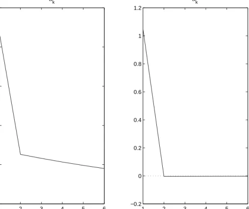
0 1 2 3 4 5 6 7 8 0 0.2 0.4 0.6 0.8 1
(a) Interest rate
optimal non−inertial nat. rate 0 1 2 3 4 5 6 7 8 −0.1 −0.05 0 0.05 0.1 0.15 (b) Inflation 0 1 2 3 4 5 6 7 8 −0.5 0 0.5 1 (c) Output gap
Figure 3: Optimal responses to an increase in the natural rate of interest. variations in the inflation rate to be optimal, even in the absence of cost-push shocks.
This leads us to consider the problem of finding the state-contingent evolution of inflation, output and interest rates to minimize the expected discounted value of (1.14) subject to the constraints (1.1) and (1.15). A similar Lagrangian method as in section 1.1 leads to first-order conditions of the form
πt−β−1σϕ1t−1+ϕ2t−ϕ2t−1 = 0, (1.16)
λx(xt−x∗) +ϕ1t−β−1ϕ1t−1−κϕ2t= 0, (1.17)
whereϕ1t is the multiplier associated with constraint (1.15) and ϕ2t the one associated with constraint (1.1). We can once again solve this system of equations for unique bounded paths for the endogenous variables in the case of any bounded processes for the exogenous disturbances{rn
t, ut}. The implied optimal responses to an exogenous increase in the natural rate of interest are shown in Figure 3. Here the model parameters are calibrated as in Table 1, and the natural rate of interest is assumed to be a first-order autoregressive process with serial correlation coefficient ρr = 0.35.15
A notable feature of Figure 3 is that once again optimal policy must be history-dependent, for the optimal responses to the disturbance are more persistent than the disturbance itself. As discussed in Woodford (1999a), optimal interest-rate policy is inertial, in the sense that interest rates are both raised only gradually in response to an increase in the natural rate of interest, and then returned to their normal level more gradually than the natural rate itself as well. (The impulse response of the natural rate is shown by the dotted line in panel 1 of the figure.) Because spending responds to expected future interest rates and not only current short rates, it is possible to achieve a given degree of stabilization of demand (relative to the natural rate) in response to disturbances with less volatility of short-term interest rates if short rates are moved in a more inertial fashion. (The optimal responses among those achievable using a purely forward-looking target criterion are shown, for purposes of comparison, by the dashed lines in the figure.)
A history-dependent target criterion that can bring about the desired impulse responses, again regardless of the statistical properties of the disturbances rn
t and ut (including any assumptions about the degree of correlation between these disturbances), can be derived once more from the first-order conditions (1.16) – (1.18). Using the last two equations to substitute for the two Lagrange multipliers in the first equation, we are left with a linear
15The real disturbances that cause the natural rate of interest to vary are assumed to create no variation in
the cost-push termut; that is, they shift the equilibrium relation between inflation and output only through
possible shifts in the natural rate of output. A variety of examples of real disturbances with this property are discussed in Woodford (2003, chap. 6).
relation of the form
A(L)(it−i∗) = φππt+φx(xt−xt−1) (1.19) that must be satisfied each period under an optimal policy. Here the coefficients of the lag polynomial are A(L)≡1− Ã 1 + κσ β ! L−β−1 L(1−L), and the inflation and output response coefficients are
φπ = κσ
λi
>0, φx = σλx
λi
>0. (1.20)
One can furthermore show that this is not only a necessary feature of an optimal equilibrium, but also suffices to characterize it, in the sense that the system consisting of equation (1.19) together with the structural equations (1.1) and (1.15) has a unique non-explosive solution, in which the equilibrium responses to shocks are optimal.16
Requirement (1.19) can be interpreted as an inertial Taylor rule, as discussed in Giannoni and Woodford (2002b). However, this requirement can also be equivalently expressed in a forward-integrated form, that more directly generalizes the optimal target criterion derived in section 1.1. It is easily seen that our sign assumptions on the model parameters imply that A(L) can be factored as
A(L)≡(1−λ1 L)(1−λ2 L), where 0< λ1 <1< λ2. It then follows that (1.19) is equivalent to
(1−λ1L)(it−1−i∗) = −λ−21Et[(1−λ−21L−1)−1(φππt+φx∆xt)], (1.21) in the sense that bounded stochastic processes {it, πt, xt} satisfy (1.19) for all t ≥ t0 if and only if they satisfy (1.21) for allt≥t0.17Hence a commitment to ensure that (1.21) is satisfied at all times implies a determinate rational-expectations equilibrium in which the responses to shocks are optimal. This conclusion is once again independent of any assumption about the statistical properties of the disturbances, so that (1.21) is a robustly optimal target criterion.
16See Giannoni and Woodford (2002b), Proposition 6. 17See Giannoni and Woodford (2002b), Proposition 7.
This optimal target criterion can be expressed in the form
Ft(π) +φFt(x) =θxxt−1−θi(it−1−i∗)−θ∆∆it−1, (1.22) where for each of the variables z =π, x we use the notation Ft(z) for a conditional forecast
Ft(z)≡
∞
X
j=0
αz,jEtzt+j
involving weights {αz,j}that sum to one. Thus the criterion specifies a time-varying target value for a weighted average of an inflation forecast and an output-gap forecast, where each of these forecasts is in fact a weighted average of forecasts at various horizons, rather than a projection for a specific future date. The coefficients of this representation of optimal policy are given by φ=θx = (1−λ−21) λx κ >0, θi =λ2(1−λ1)(1−λ−21) λi κσ >0, θ∆=λ1λ2(1−λ−21) λi κσ >0,
while the optimal weights in the conditional forecasts are
απ,j =αx,j = (1−λ2−1)λ−2j.
Thus the optimal conditional forecast is one that places positive weight on the projection for each future period, beginning with the current period, with weights that decline exponentially as the horizon increases. The mean distance in the future of the projections that are relevant to the target criterion is equal to
∞
X
j=0
αz,jj = (λ2−1)−1
In the case of the calibrated parameter values in Table 1, the rate at which these weights decay per quarter is λ−21 = .68, so that the mean forecast horizon in the optimal target criterion is 2.1 quarters. Thus while the optimal target criterion in this case involves pro-jections of inflation and output beyond the current quarter, the forecast horizon remains quite short compared to the actual practice of inflation forecast-targeting central banks. For these same parameter values, the optimal relative weight on the output-gap forecast is
φ = .04,18 indicating that the target criterion is largely an inflation target. The remaining optimal coefficients are θx = .04, θi = .24, and θ∆ = .51, indicating a substantial degree of history-dependence of the optimal flexible inflation target. The fact that θx = φ indicates that it is the forecasted increase in the output gap relative to the previous quarter’s level, rather than the absolute level of the gap, that should modify the inflation target, just as in section 1.1. The signs of θi and θ∆ imply that policy will be made tighter (in the sense of demanding a lower modified inflation forecast) when interest rates have been high and/or increasing in the recent past; this is a way of committing to interest-rate inertia of the kind shown in Figure 3.
Note that in the limiting case in which λi = 0, this target criterion reduces to (1.8). In that limit, θi, θ∆ and the decay factor λ2−1 become equal to zero, while φ and θx have a well-defined (common) positive limit. Thus in this limiting case, the optimal targeting rule is one in which the inflation target must be modified in proportion to the projected change in the output gap, but it is no longer also dependent on lagged interest rates, and the relevant inflation and output-gap projections do not involve periods beyond the current one. This will also be nearly true in the case of small enough positive values of λi.
We may similarly introduce an interest-rate stabilization objective in the case of the model with inflation inertia considered in section 1.2. In this case, the loss function (1.10) is generalized to
Lt = (πt−γπt−1)2+λx(xt−x∗)2+λi(it−i∗)2, (1.23)
18If we write the target criterion in terms of a forecast for the annualized inflation rate (4π
t), the relative
for some λi >0 and some desired interest rate i∗. In this generalization of the problem just considered, the first-order condition (1.16) becomes instead
πqdt −βγEtπt+1qd −β−1σϕ1t−1−βγEtϕ2,t+1+ (1 +βγ)ϕ2t−ϕ2t−1 = 0, (1.24) where πqdt is again defined in (1.11). Conditions (1.17) – (1.18) remain as before.19
Again using the latter two equations to eliminate the Lagrange multipliers, we obtain a relation of the form
Et[A(L)(it+1−i∗)] = −Et[(1−βγL−1)qt] (1.25) for the optimal evolution of the target variables. Here A(L) is a cubic lag polynomial
A(L)≡βγ−(1 +γ+βγ)L+ (1 +γ+β−1(1 +κσ))L2−β−1L3, (1.26) while qt is a function of the projected paths of the target variables, defined by
qt ≡ κσ λi " πqdt + λx κ ∆xt # .
The lag polynomial A(L) can be factored as A(L) = (1−λ1L)L2B(L−1), where B(L−1) is a quadratic polynomial, and under our sign assumptions one can further show 20 that 0 < λ1 < 1, while both roots of B(L) are outside the unit circle. Relation (1.25) is then equivalent21 to a relation of the form
(1−λ1L)(it−1−i∗) = −Et[B(L−1)−1(1−βγL−1)qt], (1.27) which generalizes (1.21) to the case γ 6= 0.
This provides us with a robustly optimal target criterion that can be expressed in the form
Ft(π) +φFt(x) = θππt−1+θxxt−1 −θi(it−1−i∗)−θ∆∆it−1, (1.28)
19One easily sees that in the case thatγ= 1,the only long-run average inflation rate consistent with these
conditions is ¯π=i∗−r,¯ where ¯r is the unconditional mean of the natural rate of interest. This is true for
any λi >0, no matter how small. Hence even a slight preference for lower interest-rate variability suffices
breaks the indeterminacy of the optimal long-run inflation target obtained for the caseγ= 1 in section 1.2.
20See Giannoni and Woodford (2002b), Proposition 8. 21See Giannoni and Woodford (2002b), Proposition 11.
generalizing (1.22). Under our sign assumptions, one can show22 that
φ = θx > 0, 0 < θπ ≤ 1, and
θi, θ∆ > 0.
Furthermore, for fixed values of the other parameters, as γ →0, θπ approaches zero and the other parameters approach the non-zero values associated with the target criterion (1.22). Instead, as γ →1, θπ approaches 1, so that the target criterion involves only the projected change in the rate of inflation relative to its already existing level, just as we found in section 1.2 when there was assumed to be no interest-rate stabilization objective.
The effects of increasing γ on the coefficients of the optimal target criterion (1.28) is illustrated in Figure 4, where the coefficients are plotted against γ, assuming the same calibrated values for the other parameters as before. It is interesting to note that each of the coefficients indicating history-dependence (θπ, θx, θi, and θ∆) increases with γ (except perhaps when γ is near one). Thus if there is substantial inflation inertia, it is even more important for the inflation-forecast target to vary with changes in recent economic conditions. It is also worth noting that the degree to which the inflation target should be modified in response to changes in the output-gap projection (indicated by the coefficient φ) increases with γ. While our conclusion for the case γ = 0 above (φ = .04) might have suggested that this sort of modification of the inflation target is not too important, we find that a substantially larger response is justified if γ is large. The optimal coefficient is φ = 0.13, as in sections 1.1 and 1.2, if γ = 1; and once again this corresponds to a weight of 0.51 if the inflation target is expressed as an annualized rate.
The panels of Figure 5 correspondingly show the relative weightsαz,j/αz,0 on the forecasts at different horizons in the optimal target criterion (1.28), for each of several alternative values of γ. As above, the inclusion of an interest-rate stabilization objective makes the
0 0.2 0.4 0.6 0.8 1 0 0.5 1 1.5 2 θi 0 0.2 0.4 0.6 0.8 1 0 0.5 1 1.5 2 θ∆ 0 0.2 0.4 0.6 0.8 1 0 0.2 0.4 0.6 0.8 1 θπ γ 0 0.2 0.4 0.6 0.8 1 0 0.2 0.4 0.6 0.8 1 θx [= φx] γ
Figure 4: Coefficients of the optimal targeting rule (1.28) as functions of γ.
optimal target criterion more forward-looking than was the case in section 1.2. Indeed, we now find, at least for high enough values of γ, that the optimal target criterion places non-negligible weight on forecasts more than a year in the future. But it is not necessarily true that a greater degree of inflation inertia justifies a target criterion with a longer forecast horizon. Increases in γ increase the optimal weights on the current-quarter projections of both inflation and the output gap (normalizing the weights to sum to one), and instead make the weights on the projections for quarters more than two quarters in the future less
positive. At least for low values of γ (in which case the weights are all non-negative), this makes the optimal target criterion less forward-looking.
For higher values of γ, increases in γ do increase the absolute value of the weights on forecasts for dates one to two years in the future (these become more negative). But even
0 2 4 6 8 10 12 −0.2 0 0.2 0.4 0.6 0.8 1 απ,j /απ ,0 j 0 2 4 6 8 10 12 −0.2 0 0.2 0.4 0.6 0.8 1 αx,j /α x,0 j γ = 0.1 γ = 0.3 γ = 0.5 γ = 1
Figure 5: Relative weights on forecasts at different horizons in the optimal criterion (1.28). in this case, the existence of inflation inertia does not justify the kind of response to longer-horizon forecasts that is typical of inflation-targeting central banks. An increase in the forecast level of inflation and/or the output gap during the second year of a bank’s current projection should justify a loosening of current policy, in the sense of a policy intended to
raise projected inflation and/or the output gap in the next few quarters. This is because in the model with large γ, welfare losses result from inflation variation rather than high inflation as such; a forecast of higher inflation a year from now is then a reason to accept somewhat higher inflation in the nearer term than one otherwise would.
1.4
Wages and Prices Both Sticky
A number of studies have found that the joint dynamics of real and nominal variables are best explained by a model in which wages as well as prices are sticky (e.g., Amato and Laubach, 2001b; Christiano et al., 2001; Smets and Wouters, 2002; Altig et al., 2002; and
Woodford, 2003, chap. 3). This is often modeled in the way suggested by Erceget al. (2000), with monopolistic competition among the suppliers of different types of labor, and staggered wage setting analogous to the Calvo (1983) model of price setting. The structural equations of the supply side of this model can be written in the form
πt=κp(xt+ut) +ξp(wt−wnt) +βEtπt+1, (1.29)
πw
t =κw(xt+ut) +ξw(wtn−wt) +βEtπwt+1, (1.30) together with the identity
wt=wt−1+πwt −πt, (1.31)
generalizing the single equation (1.1) for the flexible-wage model. Hereπw
t represents nominal wage inflation, wt is the log real wage, wtn represents exogenous variation in the “natural real wage”, and the coefficients ξp, ξw, κp, κw are all positive. The coefficient ξp indicates the sensitivity of goods-price inflation to changes in the average gap between marginal cost and current prices; it is smaller the stickier are prices. Similarly,ξw indicates the sensitivity of wage inflation to changes in the average gap between households’ “supply wage” (the marginal rate of substitution between labor supply and consumption) and current wages, and measures the degree to which wages are sticky.23
We note furthermore that κp ≡ξpωp andκw ≡ξw(ωw+σ−1),whereωp >0 measures the elasticity of marginal cost with respect to the quantity supplied, at a given wage; ωw > 0 measures the elasticity of the supply wage with respect to quantity produced, holding fixed households’ marginal utility of income; and σ > 0 is the same intertemporal elasticity of substitution as in (1.15). In the limit of perfectly flexible wages, ξw is unboundedly large, and (1.30) reduces to the contemporaneous relation wt−wnt = (ωw +σ−1)(xt+ut). Using this to substitute for wt in (1.29), the latter relation then reduces to (1.1), where
κ≡ξp(ωp+ωw+σ−1) (1.32)
23For further discussion of these coefficients, and explicit formulas for them in terms of the frequency of
and the cost-push shock ut has been rescaled.
Given the proposed microeconomic foundations for these relations, Erceg et al. show that the appropriate welfare-theoretic stabilization objective is a discounted criterion of the form (1.2), with a period loss function of the form
Lt=λpπ2t +λwπtw2+λx(xt−x∗)2. (1.33) Here the relative weights on the various stabilization objectives are given by
λp = θpξ−p1 θpξ−p1+θwφ−1ξ−w1 >0, λw = θwφ−1ξ−w1 θpξ−p1+θwφ−1ξ−w1 >0, (1.34) λx =λp κ θp >0, (1.35)
as functions of the underlying model parameters. Note that we have normalized the weights so thatλp+λw = 1,and that (1.35) generalizes the previous expression (1.4) for the flexible-wage case.
Here we again abstract from the motives for interest-rate stabilization discussed in the previous section. As a result, we need not specify the demand side of the model. We then wish to consider policies that minimize the criterion defined by (1.2) and (1.33), subject to the constraints (1.29) – (1.31).
The Lagrangian method illustrated above now yields a system of first-order conditions
λpπt+ϕpt−ϕp,t−1+υt= 0, (1.36)
λwπwt +ϕwt−ϕw,t−1−υt = 0, (1.37)
λx(xt−x∗)−κpϕpt−κwϕwt = 0, (1.38)
υt=ξpϕpt−ξwϕwt+βEtυt+1, (1.39)
whereϕpt, ϕwt, υt are the Lagrange multipliers associated with constraints (1.29), (1.30) and (1.31) respectively. We can again use three of the equations to eliminate the three Lagrange multipliers, obtaining a target criterion of the form
where
πasymt ≡λpξpπt−λwξwπwt is a measure of the asymmetry between price and wage inflation,
πsymt ≡
λpκpπt+λwκwπwt
λpκp+λwκw
is a (weighted) average of the rates of price and wage inflation, and
qt≡(λpκp +λwκw) " πsymt + λx λpκp+λwκw (xt−xt−1) # . (1.41)
In the special case that κw =κp =κ >0, which empirical studies such as that of Amato and Laubach (2001b) find to be not far from the truth,24 the optimal target criterion (1.40) reduces simply to qt= 0,or
πsymt +φ(xt−xt−1) = 0, (1.42)
with φ=λx/κas in section 1.1.25 More generally, the optimal target criterion is more com-plex, and slightly more forward-looking (as a result of the inertia in the real-wage dynamics when both wages and prices are sticky26). But it still takes the form of an output-adjusted inflation target, involving the projected paths of both price and wage inflation; and since all terms except the first one in (1.40) are equal to zero under a commitment to ensure that
qt= 0 at all times, the target criterion (1.42) continues to provide a fairly good approxima-tion to optimal policy even whenκw is not exactly equal to κp.
This is of the same form as the optimal target criterion (1.8) for the case in which only prices are sticky, with the exception that the index of goods price inflationπtis now replaced by an indexπsymt that takes account of both price and wage inflation. Of course, the weight
24See the discussion in Woodford (2003), chapter 3. In this case, the structural equations (1.29) – (1.30)
imply that the real wage will be unaffected by monetary policy, instead evolving as a function of the real disturbances alone. Empirical studies often find that the estimated response of the real wage to an identified monetary policy shock is quite weak, and not significantly different from zero. Indeed, it is not significantly different from zero in our own analysis in section 2, though the point estimates for the impulse response function suggest that wages are not as sticky as prices.
25Here we assume a normalization of the loss function weights in (1.33) in whichλ
p+λw= 1,corresponding
to the normalization in (1.3).
26This only affects the optimal target criterion, of course, to the extent that the evolution of the real wage
that should be placed on wages in the inflation target depends on the relative weight on wage stabilization in the loss function (1.33). If one assumes a “traditional” stabilization objective of the form (1.3), so that λw = 0, then (1.42) is again identical to (1.8). However, one can show that expected utility maximization corresponds to minimization of a discounted loss criterion in which the relative weight on wage-inflation stabilization depends on the relative stickiness of wages and prices, as discussed by Erceg et al. (2000).27
1.5
Habit Persistence
In the simple models thus far, the intertemporal IS relation (1.15) implies that aggregate demand is determined as a purely forward-looking function of the expected path of real inter-est rates and exogenous disturbances. Many empirical models of the monetary transmission mechanism instead imply that the current level of aggregate real expenditure should depend positively on the recent past level of expenditure, so that aggregate demand should change only gradually even in the case of an abrupt change in the path of interest rates. A simple way of introducing this is to assume that private expenditure exhibits “habit persistence” of the sort assumed in the case of consumption expenditure by authors such as Fuhrer (2000), Edge (2000), Christiano et al. (2001), Smets and Wouters (2002), and Altig et al. (2002).
Here, as in the models above, we model all interest-sensitive private expenditure as if it were non-durable consumption; that is, we abstract from the effects of variations in private expenditure on the evolution of productive capacity.28 Hence we assume habit persistence in the level of aggregate private expenditure, and not solely in consumption, as in the models of Amato and Laubach (2001a) and Boivin and Giannoni (2003). This might seem odd, given that we do not really interpret the “Ct” in our model as referring mainly to consumption expenditure. But quantitative models that treat consumption and investment spending separately often find that the dynamics of investment spending are also best captured by
27See also Woodford (2003, chap. 6), which modifies the derivation of Erceget al. to take account of the
discounting of utility.
28See McCallum and Nelson (1999) and Woodford (2003, chap. 4) for further discussion of this
specifications of adjustment costs that imply inertia in the rate of investment spending (e.g.,
Edge, 2000; Christiano et al., 2001; Altig et al., 2002; Basu and Kimball, 2002). The “habit persistence” assumed here should be understood as a proxy for adjustment costs in investment expenditure of that sort, and not solely (or even primarily) as a description of household preferences with regard to personal consumption.29
Following Boivin and Giannoni (2003), let us suppose that the utility flow of any house-hold h in period t depends not only on its real expenditure Ch
t in that period, but also on that household’s level of expenditure in the previous period.30 Specifically, we assume that the utility flow from expenditure is given by a function of the form
u³Ch
t −ηCth−1;ξt
´
,
where ξt is a vector of exogenous taste shocks, u(·;ξ) is an increasing, concave function for each value of the exogenous disturbances, and 0 ≤ η ≤ 1 measures the degree of habit persistence. (Our previous model corresponds to the limiting case η = 0 of this one.) The household’s budget constraint remains as before.
In this extension of our model, the marginal utility for the representative household of additional real income in period t is no longer equal to the marginal utility of consumption in that period, but rather to
λt=uc(Ct−ηCt−1;ξt)−βηEt[uc(Ct+1−ηCt;ξt+1)]. (1.43) The marginal utility of income in different periods continues to be linked to the expected return on financial assets in the usual way, so that equilibrium requires that
λt=βEt[λt+1(1 +it)Pt/Pt+1]. (1.44) Using (1.43) to substitute for theλ’s in (1.44), we obtain a generalization of the usual Euler equation for the intertemporal allocation of aggregate expenditure given expected rates of return.
29For further discussion, see Woodford (2003, chapter 5, sec. 1.2).
30Note that the consumption “habit” is assumed here to depend on the household’s own past level of