Detecting drones using machine learning

(1)

2017

Detecting drones using machine learning

Waylon Dustin Scheller

Iowa State University

Follow this and additional works at:https://lib.dr.iastate.edu/etd

Part of theDatabases and Information Systems Commons, and theLibrary and Information

Science Commons

This Thesis is brought to you for free and open access by the Iowa State University Capstones, Theses and Dissertations at Iowa State University Digital Repository. It has been accepted for inclusion in Graduate Theses and Dissertations by an authorized administrator of Iowa State University Digital Repository. For more information, please [email protected].

Recommended Citation

Scheller, Waylon Dustin, "Detecting drones using machine learning" (2017).Graduate Theses and Dissertations. 16210.

(2)

Detecting drones using machine learning by

Waylon D. Scheller

A thesis submitted to the graduate faculty

in partial fulfillment of the requirements for the degree of MASTER OF SCIENCE

Major: Information Assurance Program of Study Committee: Douglas W Jacobson, Major Professor

Thomas Earl Daniels Neil Gong

The student author, whose presentation of the scholarship herein was approved by the program of study committee, is solely responsible for the content of this thesis. The Graduate College will ensure this thesis is globally accessible and will not permit alterations

after a degree is conferred.

Iowa State University Ames, Iowa

2017

(3)

DEDICATION

I want to dedicate this to my beautiful wife Elizabeth. She has given me a ton of support throughout this whole process and I could not have done it without her.

(4)

TABLE OF CONTENTS

NOMENCLATURE iv

ACKNOWLEDGMENTS v

ABSTRACT vi

CHAPTER 1. DRONES AND HOW THEY WORK 1

CHAPTER 2. DETECTING DRONES 5

Research Methods and Analysis 7

Training the Models 14

CHAPTER 3. RESULTS 20

CHAPTER 4. SUMMARY AND CONCLUSIONS 21

REFERENCES 23

APPENDIX A LOGISTIC REGRESSION MODEL CODE 25

APPENDIX B RANDOM FOREST MODEL CODE 27

(5)

NOMENCLATURE

RF Radio Frequency

FHSS Frequency Hopping Spread Spectrum DSSS Direct Sequence Spread Spectrum

(6)

ACKNOWLEDGMENTS

I would like to thank my committee chair, Dr. Doug Jacobson, and my committee members, Dr. Thomas Daniels and Neil Gong, for their guidance and support throughout the course of this research.

In addition, I would also like to thank my friends, colleagues, the department faculty and staff for making my time at Iowa State University a wonderful experience. I want to also offer my appreciation to those who were willing to participate in my surveys and

(7)

ABSTRACT

Drones are becoming an increasing part of the ever-connected society that we currently live in. Drones are used for delivering packages, geographic surveying, assessing the health of crops or just good old fashioned fun. Drones are excellent tools and their uses are expected to expand in the future. Yet, drones can be easily misused for malicious purposes if drone security isn't taken more seriously. One of the bigger problems drones have been causing lately is that they are being used to capture images or video of disasters, such as wildfires and in doing so get in the way of the relief effort. They also have caused several problems by flying too close to airports. These drones are usually too small for radar to pick up and are often discovered by visual means and by that time it is too late. One defense against this has been GPS designated no fly zones, however, this can be easily overcome by spoofing the GPS signal to make the drone think it is in a safe area to fly.

In this paper, I examine ways of detecting the presence of a drone using machine learning models by recording the RF spectrum during a drone’s flight and then feeding the raw data into a machine learning model. This could be used around airports or even on the airplanes themselves to detect the presence and/or approach of a drone. Specifically, I examine two very popular consumer drones and their transmitters: The 3D Robotics Solo and the DJI Phantom 2. These two types of drones are unique in the way that they send and receive signals to the transmitter. I show that machine learning models, once trained, can detect drone activity in the RF spectrum. However, more work is needed in order to improve the detection rate of these models so that they may be employed in a practical manner.

(8)

CHAPTER 1. INTRODUCTION: DRONES AND HOW THEY WORK

When we think of drones most of us think of the multirotor copters that fly around, but drones can also refer to any of the powered radio controlled (RC) aerial vehicles such as airplanes or blimps. The term “drone” will be utilized in this paper to reference multirotor copters as those have become the most popular in the last few years. They are easy to fly and come in all sizes from some that will fit in the palm of your hand to ones that can carry a full-size movie camera.

Many of these drones work the same as other radio controlled devices where the controller is the transmitter and the drone has an onboard receiver to understand what the controller is sending to it. Normally, the frequency band allocated by the FCC for RC toys is either 27MHz or 49MHz while some of the hobby RC aircraft operate at 72 or 75MHz. The control frequency for the newer drones, however, will be in the 2.4GHz or 5GHz range from the manufacturer. Transmitters and receivers are available in different frequency ranges so if the drone is going to be custom built, it could be operating on a different frequency than ones listed above. Some of the more expensive drones have multiple

transmitters and receivers in different frequency bands; one for the controlling of the vehicle and one for transmitting live video or telemetry back to the operator.

One issue you will notice almost immediately with the newer drones is that Wi-Fi also operates in the 2.4GHz and 5GHz frequency range. In order to avoid interference or false command being issued to the vehicle in flight, the control signal is encoded using one of several common encoding schemes for RC vehicles. The transmitter sends a signal encoded in the specific frequency range while the receiver is constantly listening in that

(9)

frequency range with the same encoding. This way all of the Wi-Fi signals do not get interpreted by the receiver as command and cause the vehicle to crash. The encoding also prevents other people who are flying similar vehicles from taking over a vehicle with their controller. Most controllers have to be paired with a receiver as well. This prevents someone from buying a controller, setting it to the right frequency and taking over another drone/vehicle. Although that data is encoded, interference can still come from something transmitting on that frequency with a higher power level; also known as jamming.

There are several common types of encoding used by transmitters on the market. There is pulse position modulation (PPM), pulse code modulation (PCM), intelligent pulse decoding (IPD) and digital signature recognition (DRS). PPM is the oldest form of

communicating with the RC vehicle. It sends out pulses using time on the certain frequency followed by a sync pulse at the end. In short, the encoding of the message is based on time. Typically, these types of transmitters operate using a 20 millisecond “packet.” Each channel can have a long pulse of 2ms or 0ms pulse. Since common transmitters are 6 channels, the control pulses can last up to 12ms of the pulse and the sync pulse would fill out the rest of the 8ms. When flying with lots of other RC vehicles, the spectrum has to be managed to ensure that no one drone is ever on the same frequency; otherwise there will be interference with other RC operators. Older RC vehicles use the PPM type of encoding, but the newer the transmitter the more likely it uses one of the other encodings that have been discussed.

PCM is similar to PPM in that they use the same frequency, but PCM encodes the position of the servo motor as a number such as a 0 or a 1. Both PCM and PPM use the same carrier frequency but with different encodings so that the chance of interference is the same. The difference is how the interference is handled. With PPM the receiver can interpret noise

(10)

as a command and cause the vehicle problems. However, the control signal can still get partially through. With PCM, increases in interference can corrupt the signal which can lead to the receiver struggling to figure out the specific binary (1 or 0) command sent, resulting in commands being completely ignored. These are the two most common “languages” of RC vehicles. Yet, there are two additional types that must be discussed as they may be used by some of the newer types of multirotor drones.

In next two types of encoding, IPD and DRS, the vehicles have onboard processors that help tune out noise or interference and have error correction capabilities. In short, if interference does occur, the onboard processor will attempt to remedy the problem and get the control signal to its appropriate destination. These two encodings are the most secure against interference but are not immune. It is also worth noting that these signals are only encoded and are not encrypted. Understanding specific protocol and encoding being utilized will allow for better control of interference with the drone/vehicle.

The newest type of transmitter receiver combo is the spread spectrum type. This type allows the transmitter and receiver to be mated so that the receiver only ever listens to one transmitter. There is Frequency Hopping Spread Spectrum (FHSS) and Direct Sequence Spread Spectrum (DSSS). Both of these signal types are used in military applications as well as everyday items such as cell phones. Additionally, they are very resilient to interference since the transmitter and receiver are paired. The military application of this technology is used for low probability of detection (LPD) to keep the enemy from knowing that the signal is there to begin with. This makes a drone (or drones) more difficult to detect. FHSS controllers can be effective against jamming was well. This is primarily due to the fact that they are not just transmitting on a static frequency but the whole width of the spectrum the

(11)

drone is hopping in. Given adequate power, the entire spectrum can be jammed versus just a specific or static frequency.

(12)

CHAPTER 2: DETECTING DRONES

There are many different ways to detect drones, one popular way is to utilize the sound drones make from the rotors turning. The Aerospace Corporation in El Segundo, California is using acoustic microphones in combination with infrared and regular cameras to be able to detect drones [1]. They employ acoustic microphones in conjunction with cameras to be able to map the drone’s flight path in 3D. This enables them to determine possible drone configurations based on size, shape and sound; since different drone rotors make different noises [1]. They also use infrared cameras in the detection system so that they are able to detect drones in the dark. The infrared also allows them to be able to tell how long the drone has been flying based on the heat coming from the motors. Exploiting all of these mechanisms together allows them to map the drone, identify it based on signature, and even be able to tell if it’s being controlled by a pilot, GPS, or not controlled at all based on the drone’s behavior as it flies. This system was even put into use during the 2016 Rose Bowl in Pasadena [2]. Another technique is to use RADAR, but this can be problematic as some of the drones can be quite small and require specialized radar to detect them. Wi-Fi is a common detection method as some drones have identifiable service set identifier or (SSID) [3]. For example, the 3DR Solo transmitter creates a Wi-Fi network called “Sololink” followed by a number; Sololink12345. The drone knows the name of this network and has the password stored in memory so it knows which network to search for and then join. This, coupled with a default password, can be an easy way to detect and attack a drone.

Since most drones use the RF spectrum from some form of communication, including autonomous ones that are sending video back to the operator, when done reliably this is the

(13)

best way to detect drones within a certain range. Some technologies do exist to do this such as DroneDetector (http://dronedetector.com), but list no price on their website.

In this study, a HackRF software defined radio was utilized as the spectrum analyzer and a machine learning model to detect drones was employed.

When the transmitter is first turned on it does a scan of all the channels it has pre-programmed in it that it is allowed to use. Once the scan is complete it chooses the channels based on the available frequencies at that time. Then it either generates a key or has a static key that allows it to spread the transmissions out in the channels it chose in a pseudo random manner. If the key could be discovered, the generation method could be discovered, or the frequencies predicted, the transmitter will choose based on the spectrum use at that time. Then you would be able to not only detect the transmissions even though they are at or below the noise floor, you would also be able to cause interference with the transmissions since the receiver would now be able to tell the difference between the transmitter and the attacker. These are the main vectors I examined. The easiest way is to have the companies such as DJI or 3DR give the algorithms they use for frequency hopping or channel selection over to such authorities like the FAA who could use them for detection. This way detection models could be made using the exact algorithms and would have much better detection accuracy than what displayed in this paper. However, these are likely proprietary and it may be necessary to do some reverse engineering, which involves taking the drone apart down to the hardware or software and closely studying how it chooses channels as well as the way it may hop between frequencies. Yet, using machine learning would remove the prior knowledge barrier.

(14)

Research Methods and Analysis

Data was gathered from two of the more popular drone’s transmitters. The data was then utilized to teach the algorithm what drone RF signatures look like. This was

accomplished so that when the algorithm is fed new data, it knows what to look for and can find and identify drones within the spectrum.

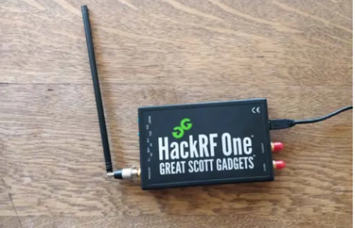
The two drones used for testing were a 3D Robotics Solo and the DJI Phantom 2. The software defined radio utilized was called the HackRF One by Great Scott Gadgets. It has a max sample rate of 20 million samples per second which limits its constant viewing of the spectrum to 20MHz. Since the 2.4-2.5Ghz range is 100MHz wide, it could not constantly view the entire spectrum. However, it can scan very quickly if the channel set is narrowed down enough. An Android Wi-Fi spectrum analyzer was also employed since it was able to pick up what channel one of the controllers showed up on. The machine learning models used for analysis of the data were written in the R programming language. Figure 1 shows what the HackRF looks like. It is a pretty simple software defined radio with an antenna, computer interface, and the red connectors for hooking multiple HackRF’s together.

(15)

The easiest way to find the operating frequencies of the transmitters is to look up the FCC ID on the transmitter. These devices have to go through testing by the FCC since they are sold in the United States.

The 3DR controller had an FCC ID of 2ADYD-AT11A. The first five characters of this ID are the Grantee ID. When you search fcc.gov using only the first five characters, it will bring up everything the particular company has applied for as far as products. Searching fcc.gov using the 2ADYD identifier brings up the 3DR controller as well as the 3DR drone itself. The far right two columns in the search show the frequencies that the items are

authorized for. In this case, the controller and the drone are authorized for communication in between 2.427 – 2.462GHz.

Figure 2: FCC ID on 3DR Solo Drone transmitter

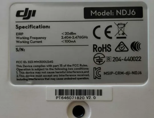
The DJI transmitter actually has the working frequency printed on the back of the controller, 2.404-2.476GHz.

(16)

Figure 3: Working frequency of DJI Phantom 2 transmitter

The next step was to collect a signal from each of the controllers while it was

operating so that the model could be trained. The model needed to have a low false positive rate when analyzing the data from the crowded 2.4GHz spectrum. This ensures that the model is actually picking up a drone rather than something else.

Starting with the 3DR Solo transmitter, I went to a local park to reduce the amount of Wi-Fi signals that would be in range of my receiver in order to reduce the amount of

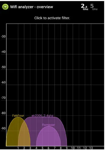
background noise when the model was trained. Initially, the Wi-Fi Analyzer smartphone app was utilized to look at what channels were currently being employed. The drone and the transmitter were then powered on to find out what channel the transmitter chose to use. Figure 4 is a snap shot of the 2.4GHz range before powering on the 3DR Solo transmitter.

(17)

Figure 4: 2.4GHz spectrum before power on of 3DR transmitter

The x-axis of the graph is the list of channels in the 2.4GHz spectrum and the y-axis is the power level of the signal in dbm. Figure 4 shows that there were only 3 Wi-Fi

networks within range of the scanner at the local park and they all had relatively low signal strengths.

(18)

Figure 5: 2.4GHz spectrum after power on of 3DR transmitter

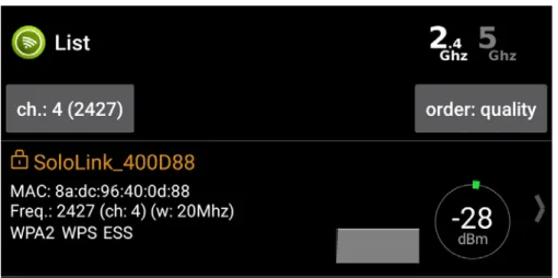
As seen in Figure 5, once the 3DR Solo transmitter was powered on, an access point named “Sololink_400D88” appeared. This is the name created for the 3DR Solo transmitter from the factory and it can be changed in a similar way a Wi-Fi router can be. Based on the channels being used and available for pickup in that area, it chose to use channel number 4. Figure 6 shows more detail on the center frequency being used by the transmitter as well as how wide the channel it was using is.

(19)

Figure 6: 3DR Solo channel details

Since the working frequency, according to the FCC, is 2.462-2.476GHz; the channel that it chose to exploit is clearly in range and using the 2.427GHz frequency with a channel width of 20MHz. Figure 6 also shows that it is using WPA2 encryption to protect the access point as well as the hardware address of this particular controller and the power level

currently detected. Since this transmitter actually creates an access point with a name for the connection, that would be the easiest way to detect if this type of drone is in the area. Now that the center frequency that the drone is using as well as the channel width is known, the HackRF One could be set to that frequency and width to collect a RF signature on this transmitter. The center frequency is 2.427, the channel width is 20MHz and the graph above shows that it is approximately evenly distributed on either side of the center frequency; making the range approximately 2.417-2.437GHz, which is well within the capabilities of the HackRF.

To capture the data needed, the HackRF_sweep command was employed. This instructs the HackRF to scan within a certain frequency range and output its scan into a csv

(20)

file which works out well since the R language likes to use spreadsheet type format for machine learning, read into the model. To run the command, you simply type “hackrf_sweep -f 2400:2490 > 3drdrone.csv” into a linux terminal. The -f option allows the selection of the upper and lower frequency ranges that are going to be scanned in MHz. The reason the whole 2.4GHz range was scanned instead of just the known range the drone operates in was because it was more advantageous to have more data available to train the machine learning model. In scanning the whole spectrum and knowing which section of the spectrum the drone was operating in, I was able to mark where I knew the drone was in the data file and allow the computer to figure out the discrepancies between where/when a drone was operating in a section of spectrum and when one was not.

Subsequently, the drone flew around the park with the hackrf_sweep command running to collect the data needed. During the flight, all of the controls on the transmitter were utilized so that as many signals as possible could be transmitted within the time the scan took place. Figure 7 shows a sample of the raw data output from the scan.

Figure 7: Sample of hackrf_sweep scan

The time is recorded along with the frequencies scanned along with the signal

strength of each signal found in that frequency range. The figure only shows two columns of signal strength data, but there is actually 51 columns of signal strength data output from the

24100000 00 00 24150000 78 -72. 27 -74. 24050000 00 00 24100000 33 -77. 72 -78. 24150000 00 00 24200000 49 -70. 74 -72. 24200000 00 00 24250000 04 -81. 23 -71. 24300000 00 00 24350000 82 -70. 98 -73. 24250000 00 00 24300000 92 -75. 95 -70.

(21)

HackRF. Figure 7 additionally shows how quickly the HackRF can perform this scan as multiple frequencies were scanned in less than a second. The total size of the file comes to about 40Mb of data which is more than enough data to train a machine learning model and get an accurate result.

When trying to attack the DJI Phantom 2 using the same procedure employed for the 3DR, it was unsuccessful. The DJI transmitter did not create a Wi-Fi network when the transmitter powered on. Additionally, I utilized the Qspectrumanalyzer app to find the spikes in the frequency range it operates in when flying, but it did not identify spikes in that part of the spectrum at all. This meant that the transmitter is either using DSSS or FHSS to hide the transmissions within the noise floor of the spectrum. Using the hackrf_sweep command, a full flight was captured from take-off to landing of the DJI drone. I then decided the trained model from the 3DR flight would be employed to try and detect the DJI drone. Even though the transmitters communicate differently, a trained machine learning model should still pick up subtle changes in the spectrum when the transmitter is communicating with the drone.

Training the Models

The next step was to go into the csv file and delete variables that have no correlation to helping the computer find where the drone is operating at such as the time. Since Figure 7 showed that the time remained the same throughout the scanning of multiple frequency buckets, it was removed for the time being. The csv file was edited to mark the sections of frequencies in which the drone was known to be operating which, as noted above, was in the range of 2.417-2.437GHz. The csv file was filtered to show only those frequencies and a column called “Drone” was added to the end. Then the “Drone” column was marked with a

(22)

1 for a yes and the rest of the frequencies where the drone was known to be not operating were marked with a 0 for no.

The prediction operations were achieved by comparing three different types of supervised machine learning classification models. The three types of machine learning models utilized were: Logistic Regression (a linear based model), Random Forest (a decision tree based model), and an artificial neural network. All of these are types of classification machine learning models. This essentially means that they are good at predicting yes or no based on prior data.

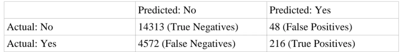
The first type of machine learning model used was a Logistics Regression model. The csv file from the collection of the 3DR drone flight had 54 columns and about 74 thousand rows. Table 1 shows the confusion matrix from this model and Table 2 shows the Accuracy, Error, False Positive rate, and the True Positive rate. Accuracy defines how often the model predicted correct. Error describes how often the machine predicted incorrectly. Moreover, the True Positive Rate illustrates how often the model was able to predict there was a drone while the False Positive Rate is how often the model predicted a drone when there wasn't one. The confusion matrix is shown as a quick reference so that accuracy can be seen promptly.

In this model, 75% of the total data was used as training data so that the model could learn how to classify whether a drone was operating or not. Conversely, the other 25% was utilized as test data to test the model in its ability to classify correctly based on what it had learned from the training data. Since the Logistic Regression model outputs probability instead of a yes or no, a simple if/else statement was used as the cutoff for the 0 or the 1. If the probability was greater that 0.5 or 50%, then the model marked it as a 1. On the other

(23)

hand, if it was less than 0.5, is was marked as a 0. The code for this model is shown in Appendix A.

Table 1: Logistic Regression Confusion Matrix from Raw 3DR Solo Model

Predicted: No Predicted: Yes

Actual: No 14313 (True Negatives) 48 (False Positives) Actual: Yes 4572 (False Negatives) 216 (True Positives)

Table 2: Logistic Regression Analysis of the Raw 3DR Solo Model

Accuracy 74.7%

Error 26.3%

True Positive Rate 4.5%

False Positive Rate 0.3%

The results from this method gave good accuracy, but a low true positive rate. This could possibly work as a decent detection algorithm. Moreover, since it is linear, it does not take up very much compute time.

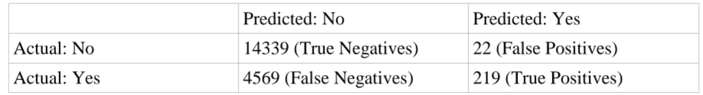
In an attempt to get a better detection rate, a Random Forrest classification model was employed next. In this model, the machine learning model is created based on decision trees. However, in the Random Forest model, many decision trees are created and vote on how the data should be classified. For example, in this case 100 decision trees were used. Therefore, the model learns from the training data 100 different times in 100 different ways. Each time it learns, the model creates a new decision tree until the max number is reached, 100 in this case. The new data that the model receives is then given to each one of the decision trees to classify. Once all of the decision trees are finished, the overall model counts each “vote”. If one tree “voted” that there was a drone flying in a certain part of the spectrum but seven trees

(24)

said there was not a drone, the model takes the majority and classifies overall that there was not a drone there. The results from this model are in Table 3 and 4 and the code is shown in Appendix B.

Table 3: Random Forest Model Confusion Matrix from Raw 3DR Solo Data

Table 4: Random Forest Analysis of the Raw 3DR Solo Model

Accuracy 75%

Error 25%

False Positive Rate .15%

This model shows about the same accuracy as the linear model, but took much longer to train and took a lot of computer time. The true positive rate is also approximately the same. The only improvement here was that the false positive rate was cut nearly in half.

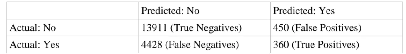
The last model employed was an artificial neural network. In this model, my code connects to an open source server farm to distribute the process of training the model and help with the compute power required for the predictions. This model works in a similar way to the decision tree model. The number of nodes desired are chosen and the nodes then try to find linkages between the data provided. Once it believes it has found those linkages that are most important to how the data ends up being classified, it assigns them a weight.

(25)

given to it based on those weights. Tables 5 and 6 show the results from the ANN training and the code is provided in Appendix C.

Table 5: Artificial Neural Network Model Confusion Matrix from Raw 3DR Solo Data

Table 6: Artificial Neural Network Analysis of the Raw 3DR Solo Model

Accuracy 73.37%

Error 26.63%

False Positive Rate 3.1%

This model has returned the best results of the three; a much better TPR and FPR. The accuracy remained about the same as the other models. This model also required a remote connection to a parallel processing server for the computer cycles that were needed to train the ANN.

To find out if the models would be able to properly detect the DJI drone flight while it is using DSSS or FHSS, the flight data from the DJI drone was fed into the Logistic Regression model, the Random Forest model, and the artificial neural network after they were trained. The results were then output into a csv file where the prediction of if the drone was there or not could be compared to the frequency that the model predicted it would be in. This way the frequencies that the models predicted a drone was in were able to be compared with the known operating frequencies of the DJI transmitter. Known false positives could

(26)

then be identified and/or controlled for and compared to known positives to rate how each model did. Two assumptions were made: 1) the other Wi-Fi routers in the park had a

negligible signal strength to affect the outcome of how the models detected the drone; and 2) the transmitter stays within the bound of its operating frequencies.

(27)

CHAPTER 3. RESULTS

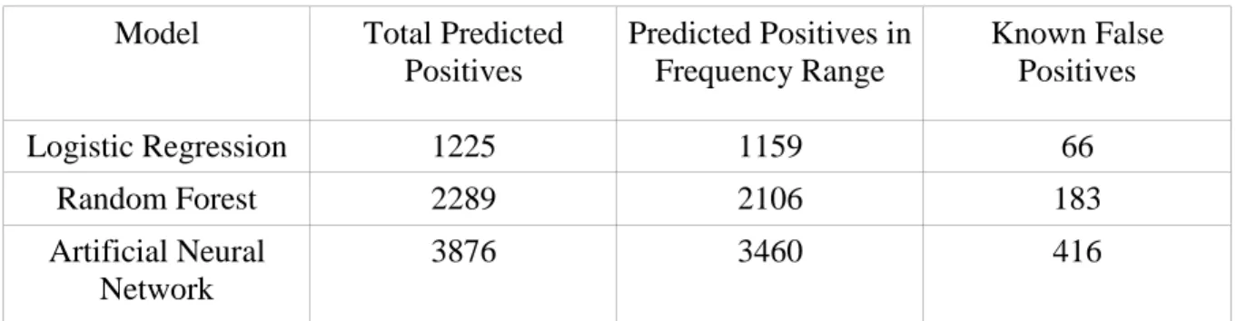
The results of each model’s detection of the DJI drone are below in Tables 7 and 8.

Table 7: Detection Results Model Total Predicted

Positives Predicted Positives in Frequency Range Known False Positives Logistic Regression 1225 1159 66 Random Forest 2289 2106 183 Artificial Neural Network 3876 3460 416

Since there was a total of 91,670 rows in the DJI flight data csv file, the detection rate was defined by how many predicted positives each model had within the operating range of the DJI transmitter over the total number of rows.

Table 8: Detection Rate

Model Detection Rate

Logistic Regression 1.26%

Random Forest 2.29%

Artificial Neural Network 3.77%

As the tables show, the model was able to detect the DJI drone even though it was using either FHSS or DSSS regardless of the model being trained to recognize a different type of RF signature from the 3DR Solo.

(28)

CHAPTER 4. SUMMARY AND CONCLUSION

In summary, once the machine learning models were trained, they were able to detect the type of drones that create their own Wi-Fi access point with a 75% accuracy. The FHSS or DSSS were still detected but with less accuracy.

I believe that with better training data or putting the data in an improved format, the model could possibly return better results. Another way to improve the model would be to change the cut off of the probability from 50% to 52-57%. This would get rid of some of the false positives, but would also lower the total detection of the DJI drone as well. A more reliable method to improve the detection of the DJI drone would be to train a machine learning model by normalizing the data in a row based on a cell that has a high signal strength in it and having a larger data set from which to work.

Some of the problems I ran into when training the models and developing the detection was the amount of processing power required to train the models as well as have the models classify the new data. The artificial neural network required connecting to a remote, open source parallel computing network to train and process the new data as well. The other two models did not require a remote connection to complete the processing, but required up to 30 minutes to process. I also could not get the data to feed into the model in real time, which would be needed when implementing this detection system near or around airports or on an airplane itself. With more processing power and a higher fidelity software defined radio such as BladRF, this could be implemented in real time or possibly throttle the amount of data being feed to the computer in real time.

(29)

In short, even though the models were able to detect the drone in a quiet benign environment, this experiment did not do testing with meaningful background noise present such as other Wi-Fi devices operating during the time the drone was operating. This research is inconclusive when using only frequency and signal strength to train the model. For this setup to be practically deployed, more work needs to be done on decoding the protocols and better pattern analysis in the data output or perhaps allowing different types of other

(30)

REFERENCES

[1] Johnson, Laura. “Aerospace Investigates Methods of Drone Detection | The Aerospace Corporation.” Aerospace, The Aerospace Corporation, 10 June 2016,

www.aerospace.org/news/events/aerospace-investigates-methods-of-drone-detection/. [2] Johnson, Laura. “Aerospace Tests Drone Detection at Rose Bowl | The Aerospace

Corporation.” Aerospace, The Aerospace Corporation, 6 Jan. 2016,

www.aerospace.org/news/highlights/aerospace-tests-drone-detection-at-rose-bowl/. [3] Richardson, Mike. “Drones: Detect, identify, intercept and hijack.” Nccgroup.trust, 2

Dec. 2015,

www.nccgroup.trust/uk/about-us/newsroom-and-events/blogs/2015/december/drones-detect-identify-intercept-and-hijack/. [4] Haken, Adam. Wi-Fi Analyzer (4.00) [Mobil Application]. Retrieved from

https://play.google.com/store/apps/details?id=info.wifianalyzer.pro&referrer=utm_so urce%3Dweb%26utm_medium%3Dpromo%26utm_campaign%3Dwfinfo

[5] Ossmann, Michael. “HackRF One.” Great Scott Gadgets, Michael Ossmann, greatscottgadgets.com/hackrf/.

[6] Ossmann, Michael. “Software Defined Radio with HackRF.” Great Scott Gadgets, Michael Ossmann, greatscottgadgets.com/sdr/.

[7] Salt, Jon. “Spread Spectrum Radios.” RCHelicopterFun.com, Jon Salt, www.rchelicopterfun.com/spectrum-radios.html.

[8] Shin H., Choi K., Park Y., Choi J., Kim Y. (2016) Security Analysis of FHSS-type Drone Controller. In: Kim H., Choi D. (eds) Information Security Applications. WISA 2015. Lecture Notes in Computer Science, vol 9503. Springer, Cham

[9] O’shea, Timothy J., T. Charles Clancy, and Hani J. Ebeid. "Practical signal detection and classification in gnu radio." Sdr forum technical conference. 2007.

[10] Shepard, Daniel P., Jahshan A. Bhatti, and Todd E. Humphreys. "Drone hack." GPS World 23.8 (2012): 30-33.

[11] Murfin, T., ed. "Fly the Pilotless Skies: UAS and UAV." GPS World 23.8 (2012): 13-15.

[12] Wesson, Kyle, and Todd Humphreys. "Hacking drones." Scientific American 309.5 (2013): 54.

(31)

[13] RStudio Team (2015). RStudio: Integrated Development for R. RStudio, Inc., Boston, MA URL http://www.rstudio.com/.

[14] Srivastava, Tavish. “How Does Artificial Neural Network (ANN) Algorithm Work? Simplified!” Analytics Vidhya, Analytics Vidhya, 20 Oct. 2014,

(32)

APPENDIX A. LOGISTICREGRESSIONMODELCODE

#importing the data

dataset = read.csv('3drdroneeditv4.csv') dataset = dataset[,5:56]

#Splitting data into training set and test set #install.packages('caTools')

library(caTools) set.seed(123)

split = sample.split(dataset$Drone, SplitRatio = 0.75) trainingset = subset(dataset, split == TRUE)

testset = subset(dataset, split == FALSE) #Feature Scaling

trainingset[-52] = scale(trainingset[-52]) testset[-52] = scale(testset[-52])

#Fitting Logistic Regression to the Training Set classifier = glm(formula = Drone ~ .,

family = binomial, data = trainingset) #Predicting Test set Results

prob_prediction = predict(classifier, type = 'response', newdata = testset[-52]) y_pred = ifelse(prob_prediction > .5, 1, 0)

#Making Confusing Matrix cm = table(testset[,52], y_pred) #Predicting DJI Drone Results djidata = read.csv('djidroneedit.csv') dataset2 = djidata[,5:56]

#Feature Scaling

dataset2[-52] = scale(dataset2[-52])

dronepredict = predict(classifier, newdata = dataset2[-52]) y_pred2 = dronepredict > 0.5

#Add prediction to the end of the djidata$Drone <- y_pred2

(33)

APPENDIX B. RANDOMFORESTMODELCODE

#Random Forest Model #data preprocessing #importing the data

#Encode Target Feature as a factor

#dataset$Drone = factor(dataset$Drone, levels = c(0,1)) #Splitting data into training set and test set

#install.packages('caTools') library(caTools)

set.seed(123)

split = sample.split(dataset$Drone, SplitRatio = 0.75) trainingset = subset(dataset, split == TRUE)

testset = subset(dataset, split == FALSE) #Feature Scaling

trainingset[, 1:51] = scale(trainingset[,1:51]) testset[,1:51] = scale(testset[,1:51])

#Fitting Random Forest to the Training Set #install.packages('randomForest')

library(randomForest)

classifier = randomForest(x = trainingset[-52], y = trainingset$Drone,

ntree = 100) #Predicting Test set Results

prob_prediction = predict(classifier, type = 'response', newdata = testset[-52]) y_pred = ifelse(prob_prediction > 0.5, 1, 0)

cm = table(testset[,52], y_pred) #Predicting DJI Drone Results djidata = read.csv('djidroneedit.csv') dataset2 = djidata[,5:56]

#Feature Scaling

(34)

dronepredict = predict(classifier, newdata = dataset2[-52]) y_pred2 = dronepredict > 0.5

#Add prediction to the end of the djidata$Drone <- y_pred2

(35)

APPENDIX C. ARTIFICIALNEURALNETWORKCODE

#ANN

#Data preprocessing #importing the data

#splitting data into training set and test set #install.packages('catools')

library(catools) set.seed(123)

split = sample.split(dataset$drone, splitratio = 0.75) trainingset = subset(dataset, split == true)

testset = subset(dataset, split == false)

#Feature Scaling

trainingset[-52] = scale(trainingset[-52]) testset[-52] = scale(testset[-52])

#fitting ann to the training set #install.packages('h2o') library(h2o) h2o.init(nthreads = -1) classifier = h2o.deeplearning(y='drone', training_frame = as.h2o(trainingset), activation = 'rectifier', hidden = c(26,26),

(36)

epochs = 100,

train_samples_per_iteration = -2)

#predicting test set results

prob_prediction = h2o.predict(classifier, newdata = as.h2o(testset[-52])) y_pred = prob_prediction > 0.5

y_pred = as.vector(y_pred)

#confusion matrix

cm = table(testset[,52], y_pred)

#predicting dji drone results

djidata = read.csv('djidroneedit.csv') dataset2 = djidata[,5:56]

#feature scaling

dataset2[-52] = scale(dataset2[-52])