Learning latent variable models : efficient algorithms and applications

(1)

Learning Latent Variable Models:

Efficient Algorithms and Applications

Matteo Ruffini

PhD program in Artificial Intelligence

Universitat Politècnica de Catalunya

Department of Computer Science

(2)

Abstract

Learning latent variable models is a fundamental machine learning problem, and the models belonging to this class – which include topic models, hidden Markov models, mixture models and many others – have a variety of real-world applications, like text mining, clustering and time series analysis. For many practitioners, the decade-old Expectation Maximization method (EM) is still the tool of choice, despite its known proneness to local minima and long running times. To overcome these issues, algorithms based on the spectral method of moments have been recently proposed. These techniques recover the parameters of a latent variable model by solving – typically via tensor decomposition – a system of non-linear equations relating the low-order moments of the observable data with the parameters of the model to be learned. Moment-based algorithms are in general faster than EM as they require a single pass over the data, and have provable guarantees of learning accuracy in polynomial time. Nevertheless, methods of moments have room for improvements: their ability to deal with real-world data is often limited by a lack of robustness to input perturbations. Also, almost no theory studies their behavior when some of the model assumptions are violated by the input data. Extending the theory of methods of moments to learn latent variable models and providing meaningful applications to real-world contexts is the focus of this thesis.

Assuming data to be generated by a certain latent variable model, the standard approach of methods of moments consists of two steps: first, finding the equa-tions that relate the moments of the observable data with the model parameters and then, to solve these equations to retrieve estimators of the parameters of the model. In Part I of this thesis we will focus on both steps, providing and analyzing novel and improved model-specific moments estimators and techniques to solve the equations of the moments. In both the cases we will introduce theoretical results, providing guarantees on the behavior of the proposed methods, and we will perform experimental comparisons with existing algorithms. In Part II, we

(3)

will analyze the behavior of methods of moments when data violates some of the model assumptions performed by a user. First, we will observe that in this context most of the theoretical infrastructure underlying methods of moments is not valid anymore, and consequently we will develop a theoretical foundation to methods of moments in the misspecified setting, developing efficient methods, guaranteed to provide meaningful results even when some of the model assumptions are violated. During all the thesis, we will apply the developed theoretical results to chal-lenging real-world applications, focusing on two main domains: topic modeling and healthcare analytics. We will extend the existing theory of methods of moments to learn models that are traditionally used to do topic modeling – like the single-topic model and Latent Dirichlet Allocation – providing improved learning techniques and comparing them with existing methods, which we prove to outperform in terms of speed and learning accuracy. Furthermore, we will propose applications of latent variable models to the analysis of electronic healthcare records, which, similarly to text mining, are very likely to become massive datasets; we will propose a method to discover recurrent phenotypes in populations of patients and to cluster them in groups with similar clinical profiles – a task where the efficiency properties of methods of moments will constitute a competitive advantage over traditional approaches.

(4)

Acknowledgements

I have to confess that writing this thesis has been quite an amazing ad-venture, which contributed to make these years in Barcelona an unforgettable time. Without doubts, this has been possible thanks to the help and the contribution of many people, that I would like to acknowledge in this note.

My first and most special thank goes to my advisor Ricard, for his patience and flexibility, for the papers that we wrote together as coauthors and for introducing me to Computer Science back in 2015. I am grateful to my amazing coauthors Marta, Borja and Guillaume for sharing with me their ideas, being willing to listen to my proposals and helping me to become a better scientist with their help and advice; and to my Master thesis advisor Giacomo, with whom I shared back in 2011 my first steps in the path of scientific research.

Combining a PhD with a full-time job in the industry is not an easy task, and it would not have been possible without the support of ToolsGroup, who encouraged me with trust and flexibility during the first years of this adventure. To all the great people working there goes a special acknowledgement, and in particular to Yossi, Eugenio – for having been a role model – to Angela and David – for their interest and curiosity toward my studies and for always pointing me great ideas and new perspectives. Likewise, I want to thank all the people in Skyscanner for sharing with me the last part of this journey, and in particular my amazing team – the Albatross squad.

My lifelong friends in Melegnano deserve a special mention for being an invaluable support during such a hard-working time, and for sharing millions of adventures across Europe that made this PhD easier and more fun.

I want to acknowledge all the institutions who provided us clinical data allowing its use for our studies – the MIMIC project, the Hospital de Sant Pau and the Catalan Health Service (CatSalut) – and all the people who helped me on the analysis and interpretation of healthcare data carried on

(5)

during this thesis: Drs. Julianna Ribera, Salvador Benito, Mireia Puig, Montserrat Busting and Esther Limón. Completing this thesis would have been way harder without the contribution of the projects and the institutions that partially funded my PhD: the projects SGR2014-890 and 2017SGR-856 (MACDA) of AGAUR (Generalitat de Catalunya); the projects

MDM-2014-0445 (BGSMath María de Maeztu Programme for Units of Excellence in R&D), TIN2014-57226-P (APCOM), and TIN2017-89244-R (MACDA) from MINECO (Ministerio de Economia, Industria y Competitividad).

I will be forever grateful to my family for always pushing me beyond my limits, to my mum Paola, my dad Marco and to my lovely grandparents who are a continuous source of inspiration.

Last, but foremost, I want to dedicate this thesis to my fiancée Francesca, for supporting me in this idea of starting a PhD, for her help in proofreading, editing and improving this thesis and for her infinite patience: I can not imagine how I could have completed this thesis without such an incredible partner.

(6)

Hierarchical Methods of Moments

113

5 A Method of Moments Robust to Model Misspecification 115 5.1 Introduction . . . 115

5.2 Existing Decomposition Algorithms and the Misspecified Setting117 5.3 Simultaneous Diagonalization Based on Whitening and Opti-mization . . . 120

5.3.1 SIDIWO in the Realizable Setting . . . 121

(8)

5.3.3 An optimal solution when l= 2. . . 128

5.4 Case Study: Hierarchical Topic Modeling . . . 129

5.4.1 Experiment on Synthetic Data . . . 131

5.4.2 Experiment on NIPS Conference Papers 1987-2015 . . 133

5.4.3 Experiment on Wikipedia Mathematics Pages . . . 134

6 Hierarchical Methods of Moments for Clustering High-Dimensional Binary Data 137 6.1 Introduction . . . 137

6.2 A data-centric Interpretation of SIDIWO . . . 140

6.3 A Hierarchical Clustering Algorithm . . . 144

6.4.1 MIMIC Dataset . . . 147

6.4.2 Tertiarism Dataset . . . 151

(9)

Abbreviations

ALS Alternating Least Square

ASVTD Approximate Singular Value-based Tensor Decomposition

D-SIDIWO Data-centric Simultaneous Diagonalization based on Whitening and Optimization

EHR Electronic Healthcare Records

EM Expectation Maximization

LDA Latent Dirichlet Allocation

LVM Latent Variable Models

MAP Maximum A Posteriori

MCMC Markov-Chain Monte Carlo

MDL Minimum Description Length

MMD Maximum Mean Discrepancy

MoM Method of Moments

SIDIWO Simultaneous Diagonalization based on Whitening and

Optimiza-tion

SVD Singular-Values Decomposition

SVTD Singular Value-based Tensor Decomposition

(10)

Introduction

Cerca una maglia rotta nella rete che ci stringe, tu balza fuori, fuggi! Va, per te l’ho pregato. Ora la sete mi sarà lieve, meno acre la ruggine

E. Montale

In our conception of the world, we are naturally led to think that what we observe around us is the result and consequence of a series of hidden mechanisms that we can not perceive. As humans, we have the ambition of understanding and explaining those mechanisms, finding meaningful models that enable us to describe, explain and predict the hidden relationship be-tween what can be observed and its latent causes.

Latent Variable Models (LVM) are a formidable tool to accomplish this need. Formally, a latent variable model is a probabilistic graphical model, designed as a set of hidden variables that influence the behavior of other observable random variables (called features). Both observable and latent variables are assumed to be random and to follow certain probability distribution; the influ-ence that latent variables play on the observable features is generally described in terms of probabilistic dependence. Latent variable models can be applied as a tool in all the fundamental tasks of machine learning, like clustering – with mixture models – time series analysis – with Hidden Markov Models and their extensions – natural language processing – with topic models – and prediction. When collecting data from reality, it is common to perform hypotheses on the intrinsic mechanisms governing their generation; these assumptions hypothesize that reality can not behave in totally arbitrary ways – a scenario where no prediction nor modeling would be possible – but follows some mech-anisms, that make it, to certain extent interpretable and predictable. Latent

(11)

variable models are synthetic tools to describe these mechanisms. Learning

a latent variable model means to find a model that properly describes the process that governs the generation of the data that we are observing. This task is commonly performed by algorithms that take as input a set of observed data, in terms of observable variables, and return an hypothesized model that properly describes them. Algorithms can come with different levels of com-plexity: the structure of the model may be known completely – leaving to the algorithm only the duty of estimating the parameters of a model – or partially, with the algorithm that also has to estimate part of the structure of the model. Recent technology development has boosted the generation of massive datasets, characterized by thousands of observable features and millions of observations. Learning algorithms for latent variable models need to be able to deal with these kind of data, returning meaningful models in conveniently short running time. Providing algorithms to learn latent variable models is the objective of this thesis. In particular, our focus will be on learning techniques able to run efficiently on massive high dimensional datasets, maintaining the guarantee of returning provably good models. We will study algorithms for several latent variable models in various different scenarios, from the case when the structure of the model is assumed known, and the algorithm is required to retrieve only the parameters of the model, to the case when some information is missing, and the algorithm is required to retrieve a meaningful model with only partial information.

The standard approach to learn a parametric LVM is based on maximum likelihood principle, and consists of finding the model that maximizes the likelihood of the observed data. Given a dataset

X ={x(1), ..., x(n)}

the maximum likelihood approach first assumes data to be generated by a certain probability distribution _P[X|Θ] – depending on a set of unknown parameters Θ– and then it looks for the value ofΘ maximizing the likelihood:

ΘM L = argmax Θ P [X |Θ] = argmax Θ n Y i=1 P[x(i)|Θ].

This approach is theoretically appealing, but it comes with several complica-tions: the likelihood function is in general non-convex, and admits closed-form

(12)

solutions only for trivial models. During the years, several heuristics have been designed to approximatively maximize the likelihood. For many decades, the standard approach to accomplish this task has been the Expectation Maximization (EM) method (Dempster et al., 1977), an heuristic that is easy to implement, but is known to be prone to poor local optima. Furthermore, EM requires several passes across the entire dataset at each iteration, which makes it unusable with massive high-dimensional datasets (Balle et al., 2014). EM is not always applicable, as complex models do not allow an explicit calculation of the likelihood function; for these cases approximate inference approaches have been developed, which have similar limitations to those of EM. Some methods are based on Monte Carlo sampling, and are computa-tionally demanding. Others are based on convex relaxations of the objective functions to be optimized, consequently returning suboptimal models. To overcome these limitations, in recent years a new framework to learn latent variable models emerged: the Method of Moments (MoM). Instead of explicitly relying on the probability density function of a model, methods of moments work by finding equations that relate the low order moments of the observable data with the parameters of the latent variable model that one wants to learn, and solving these equations typically employing tensor/matrix factorization techniques. Compared to EM, moment-based algorithms provide a stronger theoretical foundation. In particular, it is known that in the setting where data is generated by a given model, whose characteristics are known to the user – a setting called the realizable setting – the output of a method of moments will converge to the true parameters of the model as the amount of training data increases. Furthermore, MoM algorithms only make a single pass over the training data, they are highly parallelizable and they always terminate in polynomial time. These promising characteristics make methods of moments the ideal learning framework for the challenging settings that we have in mind, as MoM allows to deal with massive datasets with guarantees of retrieving a meaningful model. The theory of methods of moments to learn latent variable models will be the core focus of this thesis.

The first part of this thesis studies methods of moments when data is assumed to be generated by a known latent variable model, whose parameters are to be estimated. This is the standard setting in which methods of moments are traditionally employed. Once a latent variable model has been designed, the learning procedure consists of two steps: first, finding the equations that

(13)

relate the moments of the observable data with the model parameters and second, to solve these equations to retrieve estimators of the parameters of the model. In this part of the thesis we will focus on both steps, providing and analyzing novel estimators for the moments and novel techniques to solve the equations that allow to retrieve, from the moments, the model parameters. The second part of the thesis focuses on methods of moments when some of the information about the model generating the data is missing, or not properly specified by a user. In this context, we will observe that most of the theoretical infrastructure underlying methods of moments is not valid anymore – a fact that limits the applicability of methods of moments in scenarios where the model generating the data is unknown or misspecified, like it commonly happens with real-world data. The objective of the second part of this thesis will thus be to develop theoretical foundations to methods of moments in the misspecified setting, developing efficient methods, guaranteed to provide meaningful results even when some of the model assumptions are unknown or violated.

Despite the huge number of applications of latent variable models to real-world problems, the adoption of methods of moments is still limited, and practitioners still prefer to use more traditional approaches, like EM or ap-proximate inference methods. Providing stable and accurate MoM algorithms and pioneering their usage in a real experimental framework are thus two strictly related research goals. For this reason, during all the thesis, we will apply the developed theoretical results to challenging real world applications, focusing on two main domains: text mining and healthcare analytics.

Text mining is a discipline of natural language processing that aims at finding latent topics in text corpora. Here, the observable data, generally coincides with the words appearing in a document, while the hidden variable can be, for example, the topics with which each document is dealing. Datasets in this discipline tend to be large – with several texts in it – high-dimensional – as the vocabularies contain thousands of words – sparse – especially for corpora with just short texts likes feeds, tweets or medical annotations. These characteristics, make the traditional approaches based on the likelihood prin-ciple difficult to apply efficiently, while they constitute the ideal application scenarios for methods of moments. During the thesis we will apply methods of moments to learn models that are traditionally used to do topic modeling, comparing them with more traditional approaches.

(14)

Healthcare analytics also constitute a natural application field for latent variable models: every time a patient visits an healthcare center, a record is produced, containing for example clinical findings and prescriptions. In this context, data represents the observable manifestation of a hidden status, representing the true, unobservable status of patient’s diseases. Similarly to text mining, healthcare records are very likely to become massive datasets, with several dimensions associated to millions of patients, where the efficiency properties of methods of moments constitute a competitive advantage over traditional approaches. In this thesis, we will apply methods of moments to learn latent variable models able to provide a latent representation of patient statuses, allowing to discover recurrent phenotypes in populations of patients and to cluster patients in groups with similar clinical profiles.

Research Problems and Related Works

The seminal works on learning latent variable models with methods of moments date back to the years around 2010, when the machine learning community started realizing that a frequentist approach exploiting the mo-ments could help solving problems that where known to be intractable if faced with traditional likelihood-based approaches. Generalizing an approach intro-duced by Pearson (1894), methods of moments first store in multidimensional tensors the low-order moments of the observable data, and then recover the parameters of the desired model via tensor decomposition techniques. The idea produced several early applications for Markov models (Chang, 1996), evolutionary trees (Mossel and Roch, 2005), mixture models (Feldman et al., 2006) and multi-view models (Chaudhuri et al., 2009), finding a more explicit formalization in the subsequent works by Hsu et al. (2012); Hsu and Kakade (2013); Anandkumar et al. (2012b) and Anandkumar et al. (2012a).

Anand-kumar et al. (2014) presented an exhaustive survey showing that spectral learning of most of the LVMs can be abstracted in two steps: first, given a prescribed LVM, they show how to operate with the data to obtain an empir-ical estimate of the moments, expressed in the form of symmetric low rank matrices and tensors; in a second step, the moments are decomposed using tensor/matrix decomposition techniques, to obtain the unknown parameters of the model. That paper also recalls and studies a method to derive such decomposition, the Tensor Power Method (TPM). This abstraction allows to split the research on methods of moments in two main non-disjoint areas.

(15)

A first area concentrates on methods to retrieve from data empirical es-timates of the moments for specific LVMs. Examples are the works by Jain and Oh (2014) for mixture models with categorical observations, by Chaganty and Liang (2013) for mixtures of linear regressions, by Anandkumar et al. (2012b) for naive Bayes models, and by Hsu et al. (2012) for hidden Markov

models. Important examples come from text mining, where equations to retrieve a moment representation for the single-topic model are provided by Anandkumar et al. (2012b) and Zou et al. (2013). An alternative and more complex model is Latent Dirichlet Allocation (LDA) (see Griffiths and Steyvers, 2004; Blei et al., 2003), for which Anandkumar et al. (2012a) provide empirical estimators of the moments.

A second research area focuses on methods to decompose the low-order moments to retrieve the parameters of the model. Literature on tensor decom-position is vast and it is believed to originate from the works by Hitchcock (1927, 1928). The topic received attention in the field of psychometrics

(Car-roll and Chang, 1970; Harshman, 1970; Tucker, 1966) and chemometrics (Appellof and Davidson, 1981) and extensive surveys are provided by Tomasi and Bro (2006); Kolda and Bader (2009) and Sidiropoulos et al. (2017). These works also present several classical techniques to obtain the so-calledcanonical polyadic decomposition (CPD) of a three dimensional tensor, which expresses it as a linear combination of rank-1 tensors. Kolda and Bader (2009) recall one of the most popular algorithms to obtain the CPD of a generic tensor: Alternating Least Square (ALS) (whose origins traces back to Carroll and Chang, 1970; Harshman, 1970). ALS is an heuristic that works by fixing all-but-one of the factors decomposing a tensor, and updating the remaining factor by solving an overdetermined linear least squares problem. ALS is easy to implement and to understand but is known to be prone to local minima, requiring several random restarts to return meaningful results (see the discussion by Kolda and Bader, 2009, pg. 18). A different line of work consists in approaching the tensor decomposition problem with simultaneous Schur decompositions (Van Der Veen and Paulraj, 1996; De Lathauwer et al., 2004; Colombo and Vlassis, 2016) or matrix optimization methods to perform simultaneous diagonalization (Kuleshov et al., 2015). In theory, one could use any of these methods to decompose the three-dimensional tensor containing the third-order moments, but the high dimensionality of that tensor makes this approach often computationally unfeasible. On the other hand, one

(16)

can rely on the specific structure of the whole set of low-order moments by using not only the third, but also the first and the second order moments to explicitly exploit their symmetry properties and obtain the desired model parameters more efficiently and with provable guarantees of global optimality. This is the approach followed by methods of moments.

The reference method here is the Tensor Power Method (TPM) from Anand-kumar et al. (2014). TPM manipulates the low-order moments to obtain a symmetric orthogonal tensor that is decomposed using a high-dimensional extension of the well-known matrix power method, with an approach pro-posed by Zhang and Golub (2001) and Kolda (2001). The main issue of this algorithm is its scalability, since its running time grows as k5 _where _k

is the number of latent components. An alternative, which in general has better dependence on the number of latent factors, consists in using matrix-based techniques and a simultaneous diagonalization approach, specializing an approach that can be traced back to Sanchez and Kowalski (1990) and Leurgans et al. (1993). Examples of these methods of moments are provided by Anandkumar et al. (2012b), with an algorithm based on the eigenvectors of a linear operator; Anandkumar et al. (2012a) also present an alternative method based on the singular vectors of a Singular-Values Decomposition (SVD). These two methods are faster than TPM by far, but they are more

sensitive to perturbations on the input data.

A method of moments uses a set of n samples to empirically estimate the moments and then uses tensor decomposition methods to recover the model parameters from the decompositions of the estimated, perturbed, moments. Methods of moments can thus be improved by improving the convergence rate of the estimators – obtaining better moments with smaller sample sizes – by working on the decomposition algorithms to reduce their sensitivity to input perturbations – returning better model parameters when the input moments are perturbed – and improving their performance – performing the decompositions in shorter running times. In this thesis, we will focus on all these aspects, working on novel moment-estimators for several latent variable models and providing improved tensor decomposition techniques that allow to recover, from an estimation of the moments, robust estimates of the parameters of a latent variable model in short running times.

(17)

variable models is based on the maximum-likelihood principle and aims at finding the model that maximizes the likelihood of an observed dataset. How-ever, maximizing the likelihood is a difficult task even for simple models: Arora et al. (2012) for example proved that maximum likelihood estimates for the single topic model are NP-hard, while Roch (2006) proved the same for latent trees. Consequently, several heuristics have been developed aiming at solving the maximum likelihood problem under an approximate point of view. Expectation Maximization (Dempster et al., 1977), for example is an iterative technique that, starting from a user defined initialization (typically random), iteratively updates the parameter of a model, increasing the likelihood at each iteration. EM has only local guarantees of convergence, but is easy to understand and to implement, which makes it the most used technique in this field. Furthermore, EM requires the complete calculation of the posterior distributions, which may not be feasible for models with a complex structure; in this case it is common to use approximate inference approaches based on variational inference or Monte Carlo-based approaches (see Bishop 2006 for a detailed presentation of these techniques). Approximate inference techniques are widely used in tasks like topic modeling (Blei et al., 2003; Griffiths and Steyvers, 2004) and mixture-models learning (Marin et al., 2005). Thanks to their flexibility, they allow to deal with complex models, but, unlike methods of moments, they fail to provide optimal models in small running times. Methods of moments and likelihood-based techniques aim at the same purpose – retrieving the parameters of a model – following two different frameworks.

However, these two frameworks are not unrelated, but complementary. For example, empirical studies indicate that initializing EM with the output of a MoM algorithm can improve the convergence speed of EM by several orders of magnitude, yielding a very efficient strategy to accurately learn latent variable models (Balle et al., 2014; Chaganty and Liang, 2013; Bailly, 2011). In the case of relatively simple models this approach can be backed by intricate theoretical analyses (Zhang et al., 2014), showing that initializing EM with the output of a method of moments can provide guarantees of global optimality.

Despite their theoretical appeal, the practical applications of methods of moments are still limited, and EM remains the tool of choice of most of practitioners, notwithstanding the slow running times and the well-known proneness to poor local optima. While this is partially due to the novelty of

(18)

the MoM framework, there are also deeper theoretical issues that limit the robustness of these methods in real-world applications. Methods of moments in fact, to work with guarantees, require the user to know the exact structure of the latent variable model that he wants to learn; this means knowing the number of latent variables of a model, their distribution, and their proba-bilistic relation with observable data. However, most of these characteristics, are by definition unknown to the user, who can only estimate them with cross-validation techniques. Kulesza et al. (2014) demonstrated that when the number of latent states imposed by the user is not enough to describe the training data, a MoM can lead to unexpected results, and provided in a subsequent work (Kulesza et al., 2015) potential ways to overcome this issue. In general, it is possible to demonstrate (see Chapter 5) that when the characteristics of the model generating the data are unknown or misspecified, most of the traditional methods of moments provide no guarantees on their results. Furthermore, for methods of moments to work properly, it is crucial to deal with moments whose expectations are in a prescribed relation with respect to the parameters of the model one wants to learn; however, efficient formulations of the moments are known only for few, simple, latent variable models, requiring heavy assumptions on the data, that are systematically violated in real world scenarios. The problem of the applicability of methods of moments in settings where the model generating the data is unknown or not properly specified is largely unstudied; in this context, the traditional approach consists of refining the results of a MoM with EM, so to obtain a parameter that, at least locally, is guaranteed to be meaningful, locally maximizing the likelihood. While this approach is effective in practice, a theory on why in the misspecified setting a MoM would return a meaningful model (and thus a good initializer for EM) is still not present. Providing a theoretical analysis of methods of moments in the misspecified setting is one of the objectives of this thesis.

Overview of contributions

The first part of this thesis (Chapters 1 to 4) is dedicated to the theory of methods of moments for learning latent variable models when all the characteristics of the model generating the data are known, and only the parameters of that model need to be recovered.

(19)

Chapter 1 is dedicated to recalling the basis of methods of moments. We will present how methods of moments work by presenting a simple application for learning Naive Bayes Models with Poisson-distributed features. We will show how it is possible to recover a set of equations that relate the low-order moments of the observable data with the parameters of the model and we will then present the most used techniques to solve these equations – namely the tensor decomposition methods from Anandkumar et al. (2012b, 2014), and Alternate Least Square (Kolda and Bader, 2009). We will conclude the chapter with a brief discussion on how this approach can be generalized to any latent variable model, and on the conditions required to guarantee the identifiability of a model in this setting.

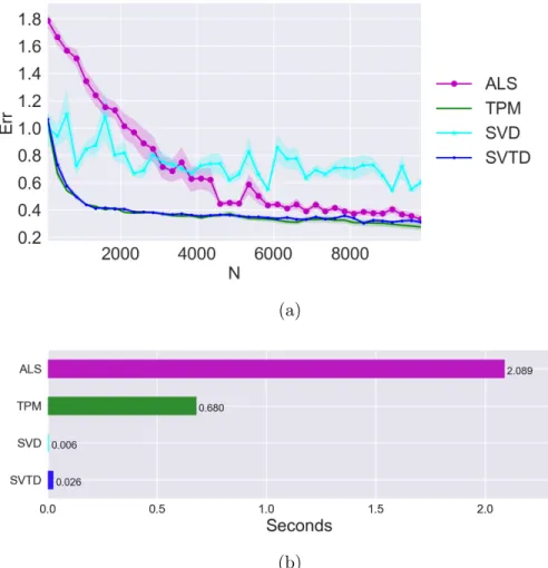
A fundamental part in methods of moments is the step that decomposes the matrices/tensors containing the moments to retrieve an estimate of the parameters of the model generating the data. This step is generally accom-plished using algorithms that employ matrix/tensor decomposition methods, which ideally are required to run in short running times and to guarantee good robustness to random perturbations – providing good learning accuracy when only a limited amount of data is available. A scan of the literature for these methods present some alternative tools of choice: Anandkumar et al. (2012a,b) present methods with high scalability, but poor robustness to perturbations, while Anandkumar et al. (2014) introduce a method with better robustness but significantly worse running times. At the same time, existing methods from tensor factorization theory (see for example Tomasi and Bro 2006; Kolda and Bader 2009; Sidiropoulos et al. 2017) provide heuristics with a worse computational complexity and less guarantees on the learning accuracy. These limitations of existing methods led us to search for an algorithm with high learning accuracy and strong efficiency guarantees. In Chapter 2 we provide a novel algorithm for the simultaneous solution of moment equations that allows to retrieve, from estimates of the moments, a set of estimates of the model parameters. This algorithm will rely on simple matrix operations – being consequently fast – and will guarantee a best-in-class learning accuracy. We will analyze the proposed method under the theoretical point of view, studying its computational complexity and its robustness to random pertur-bations of the input. Finally we will experimentally compare the proposed method with existing techniques, showing that the proposed algorithm out-performs each existing method either in terms of speed or in learning accuracy.

(20)

One of the areas where latent variable models find a natural field of ap-plication is natural language processing and topic modeling. In this field, the observable variables are the words appearing in a text, while the latent variables are the topics with which a text is dealing. A simple model is the

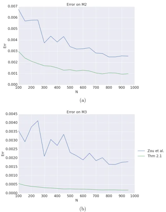
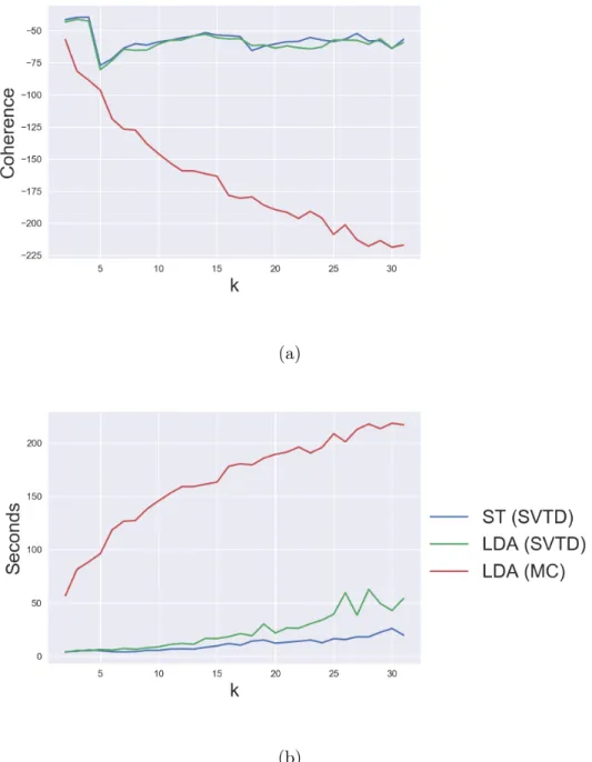
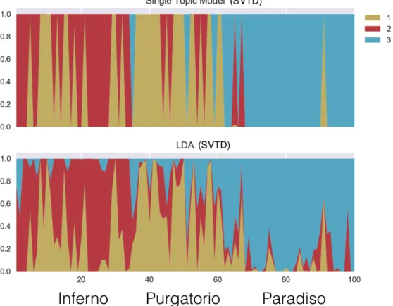
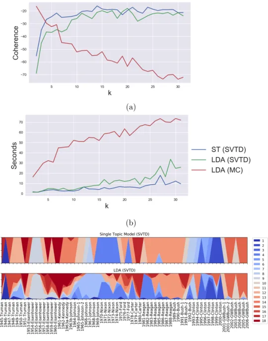
single-topic model, where each text is assumed to be about only one topic and the probability of a given word appearing in a text depends on the topic of the text. An alternative and more complex model is Latent Dirichlet Allocation (LDA) (see Griffiths and Steyvers, 2004; Blei et al., 2003), where each text is assumed to deal with a multitude of topics, and each word of a text is assumed to be associated to a unique topic. Learning techniques for topic modeling are in general dominated by Bayesian approaches, with techniques based on Markov Chain Monte Carlo methods (Griffiths and Steyvers, 2004) and variational techniques (Blei et al., 2003). At the same time, methods of moments exist to learn standard models like the single-topic model (Anand-kumar et al., 2012b; Zou et al., 2013) and LDA (Anand(Anand-kumar et al., 2012a). In Chapter 3 we present novel methods of moments to learn these two models aiming at improving existing ones. In particular we will introduce new of esti-mators of the moments for the single-topic model and for LDA, studying their sample complexity and providing novel sample complexity bounds. We will show, both experimentally and with a theoretical analysis, that the proposed estimators have an improved robustness in comparison with existing ones. Furthermore we will compare the proposed approaches with the standard Bayesian approach proposed by Griffiths and Steyvers (2004) on real-world text corpora, both for single-topic model and LDA. We will show that the moment-based method presented in this chapter recovers higher-quality topics in much smaller running time.

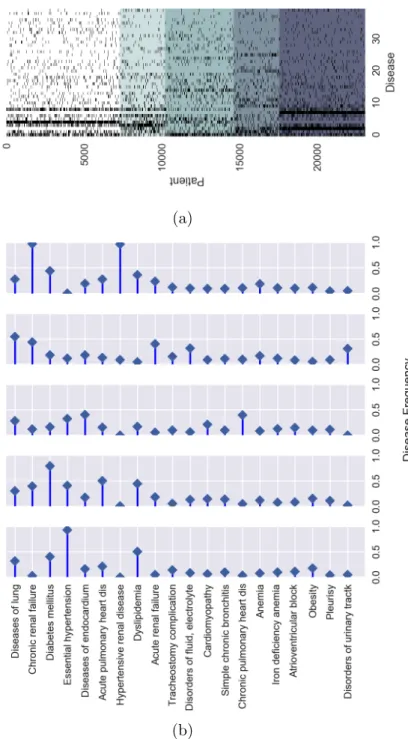
In Chapter 4 we will present an application of latent variable models to healthcare analytics, focusing on the specific task of patient clustering. We will consider the most simple kind of electronic healthcare records – namely ICD9 records (Geraci et al., 1997) registering patient diagnostics – and we will use these data with two objectives: clustering patients in groups with homogeneous clinical profiles and retrieving meaningful phenotypes – i.e. abstract representations describing the most recurrent diseases-patterns in patient statuses. To accomplish this task we will model our data as mixture models, learn the mixture with a method of moments and use that mixture to cluster the various patients, using a model-based clustering approach (Marin et al., 2005). The choice of a model-based approach over the more traditional

(21)

distance-based methods like k-means (Macqueen, 1967) or spectral clustering

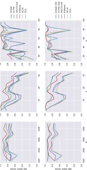
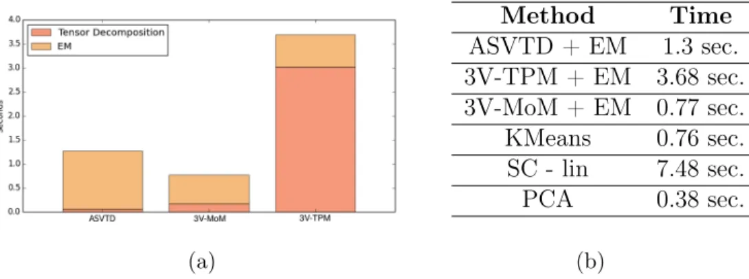
(Ng et al., 2002) has two benefits: first it allows to deal with high-dimensional sparse data, as it will be the case for our dataset, and second it provides a meaningful generative model for our dataset, allowing an easy construc-tion of phenotypes. The task of performing a moment-based learning of a mixture model will come with a peculiar challenge, because no efficient moment-estimators are known for such kind of latent variable models. As a consequence, we will propose an approximate approach where we will develop moment-estimators that are provably almost-unbiased – i.e. with a bias that can be calculated and is provably small – and feed a decomposition algorithm with these estimators. The resulting parameters will then be refined with EM, in order to remove the bias inherited from the moment estimation. We will see that this hybrid MoM-EM approach will work effectively, with EM rapidly converging to good optima. Furthermore, it will allow to present an efficient implementation of the decomposition method presented in Chapter 2, allowing it to run with a better computational complexity. We will apply this approach to the considered dataset of patients obtaining clusters and phenotypes that make sense under the clinical point of view. Furthermore, we will compare on synthetic data our approach with more traditional clustering algorithms, outperforming them in terms of clustering accuracy.

In all the chapters above we have focused on scenarios where data was generated by a latent variable model whose structure was assumed to be known to the user, and the task of a learning algorithm was reduced solely to recovering the parameters of the model. Methods of moments require the user to explicitly know the structure of the latent variable model that he wants to learn, as this information is explicitly used in two points: one is when the moment are calculated, as the formulation of the moment estimators depend on the specific model generating the data; different model will have different estimators. The second is in the decomposition algorithm, where a user needs to ask for a specific number of latent states to be returned by the algorithm. All the theory of methods of moments has been developed in therealizable

setting where the model characteristics are known to the user, and data does not violate any model assumption. This approach allowed to build a clear and round theoretical framework for methods of moments, but also limited the theoretical reliability of these methods in real-world scenarios, where the model generating the data is always unknown, and model assumptions are sure to be violated. In the second part of this thesis (Chapters 5 and 6), we

(22)

will concentrate on analyzing methods of moments when data does not follow a model of the mathematical form assumed by the algorithm, violating some of the assumptions that the user makes.

In Chapter 5 we will focus on the scenario where a method of moments is required to learn a latent variable model from data, but the number of latent states required by a user is too small to accurately represent the training data. This is a very common scenario, in particular when data is high-dimensional and it is difficult to find a number of latent states to compre-hensively describe the dataset, or this number is too high to be estimated. For example, an important application of low-dimensional learning comes from exploratory data analysis, where a mixture model with two states is required to bisect a dataset into two well-distinct classes. The desired behavior of a learning technique when run in a low-dimensional setting, is to return a small model that synthetically describes the data, providing the optimal low-dimensional model approximating the data we are observing. In Chapter 5 we will demonstrate that this is not the behavior of existing methods of moments, which instead are likely to return unexpected results when plugged with a misspecified number or latent states. As a consequence, we provide a novel decomposition algorithm for method of moment, that phrases the decomposition task as a non-convex optimization problem and generalizes the method presented in Chapter 2. We demonstrate that the proposed algorithm, when run in a low-dimensional setting, returns the optimal low-dimensional model approximating the one generating the data, according to an intuitive definition of optimality. Starting from these remarks, we apply this method to hierarchically learn latent variable models, starting with a simple, two-dimensional model, which is then refined iterating the learning step on each of the retrieved dimensions. The hierarchical nature of this method allows for a fast and accurate solution of the optimization problem raising in the decomposition task, based on low-dimensional grid search. An immediate application of this approach is to perform hierarchical clustering, where a mixture with two classes is learned, used to bisect our dataset, and then the procedure is iterated on each of the two retrieved clusters. In this chapter we will also present an application of this approach to natural language processing, providing a specialization of our method to perform hierarchical topic modeling.

(23)

come with the assumption that a user is able to calculate unbiased estimators of the moments, that asymptotically exhibit a prescribed relation with the parameters of the model. However, this assumption is possible only when data is accurately described by a latent variable model of known structure, while when the structure of the model is not known or no finite model accurately describes the data – as it is the case in real-world scenarios – nothing is known on the asymptotic behavior of the moment equations. Consequently, the theoretical infrastructure guaranteeing that methods of moments will return a good model approximating the data, loses most its strength in real-world contexts. In Chapter 6 we demonstrate that theoretical guarantees on the behavior of methods of moments can be retrieved also when no hypotheses on the model generating the data are made. In particular, we will consider a simple calculation formula for the moments, and we will demonstrate that the decomposition technique introduced in Chapter 5 provides a meaningful relation between the input data and the output model, regardless the model generating the data. This means that its output will accurately describe the data, even if the user imposes no hypotheses on the input data. Additionally, we will analyze the cost function of the considered method and its action on the input data, observing that it automatically suggests a rule to split them into meaningful clusters. From this observation, we will introduce a novel model-independent clustering algorithm that will be particularly suitable for high-dimensional binary data. We will thus apply this approach to the medical records studied in Chapter 4, obtaining meaningful hierarchical phenotypes and clinically reasonable trees of clusters.

The last chapter concludes this work and highlights the main research chal-lenges emerging from the problems faced in this thesis. Some of them are theoretical and aim at improving our current understanding of methods of moments, studying the relations that link this family of techniques with traditional likelihood-based methods. Some others are applied, and focus on extending the applicability of methods of moments to real-world scenarios.

(24)

Publications derived from the thesis

The following papers have been written as an outcome of this thesis.

• Ruffini, M. (2018). Hierarchical Methods of Moments for Clustering High Dimensional Binary Data. Submitted

• Ruffini, M., Casanellas, M., and Gavaldà, R. (2018). A new method of moments for latent variable models. Machine Learning, 107(8-10):1431– 14551

• Ruffini, M., Rabusseau, G., and Balle, B. (2017b). Hierarchical methods of moments. InNeural Information Processing Systems, pages 1901–1911

2

• Ruffini, M., Gavalda, R., and Limon, E. (2017a). Clustering patients with tensor decomposition. In Machine Learning for Healthcare Conference, pages 126–146 3

1_{https://mruffini.github.io/assets/papers/method-moments-LVM-preprint.}

pdf

2_{http://papers.nips.cc/paper/6786-hierarchical-methods-of-moments.pdf} 3_{http://proceedings.mlr.press/v68/ruffini17a/ruffini17a.pdf}

(25)

(26)

Part I

Methods of Moments for

(27)

(28)

Chapter 1

Background: Methods of

Moments

In this chapter we present the basis of Method of Moments. We begin by introducing a simple family of latent variable models called naive Bayes models and show how to learn them with methods of moments, presenting an overview of the state-of-the-art approaches. We will then show how the proposed technique can be extended to several other models.

1.1

Naive Bayes Models

A naive Bayes model is a latent variable model characterized by d+ 1

random variables (Y, X1, . . . , Xd) with the following characteristics:

• Y is a hidden (unobservable) discrete variable with a finite number of possible outcomes: Y ∈ {1, . . . , k}. We define

ωj =P(Y =j), ω= (ω1, . . . , ωk)∈∆k−1,

where∆k−1 is the k−dimensional simplex:

∆k−1 ={(π1, ..., πk)∈Rk: X

πi = 1}.

The entries of the vectorω are commonly named the mixing weights of the model.

(29)

• The vector X = (X1, . . . , Xd)is observable, its distribution depends on

the value of the hidden variableY and the random variablesX1, . . . , Xd

are conditionally independent given Y. It is common to call the entries ofX thefeatures of the model, and their conditional probability density functions may follow any parametric distribution:

Distr(X|Y =j)≈_Pj[X], Distr(Xi|Y =j)≈Pj,i[Xi].

A special role is played by the conditional expectations of the features: µj =E[X|Y =j]∈Rd, µj,i=E[Xi|Y =j]

M = [µ1|, ...,|µk]∈Rd×k.

The vectorsµ1, ..., µk are commonly called centers of the model.

Remark 1.1.1. The value ofd typically represents the amount of observable information, while the value k represents the number of latent states that are enough to provide a synthetic description of the data generated by the model. Even if d and k can take any value, during this thesis we will be mostly interested in the case of high-dimensional models, where d≥k. The generative process determined by a naive Bayes model, first generates an unobservable outcome for Y, say j, and then generates a set of observations X1, . . . , Xd, whose distribution depends on the value of Y. The conditional

independence of the features allows the following simple factorization of the probability density function:

P[X1, . . . , Xd] = k X j=1 ωjP[X1, . . . , Xd|Y =j] = k X j=1 ωj d Y i=1 Pj,i[Xi].

Naive Bayes models are a family of latent variable models, and their spe-cific distribution depends on the special characteristics of the conditional distributions of the features, namely the probability density function _Pj,i[·].

1.1.1

Learning Naive Bayes Models

In the most generic scenario, each _Pj,i is a specific probability density

function following a certain probability distribution and depending on a certain set of parameters Θi,j:

(30)

The knowledge of the distributional properties of _Pj,i, together with the

number of latent states k, constitute the probabilistic structure of the model, and we will abstract it with the notation _S. In general, this information will not be observable from a dataset, and constitutes the model assumption that a user does on the data that he is observing.

The union of all the parameters Θi,j characterizing each distribution Pj,i,

together with the mixing weights ω, constitute the set of parameters of the model, and it will be denoted with the pair (Θ, ω), where Θ ={Θj,i}j,i. Also

the parameters of the model will not be directly observable from data, but unlike the model structure, they will not be imposed by the user, as they will be the object of a learning process. Consider for example a dataset X, and impose then the model assumption that data is generated by a naive Bayes model with a certain structure _S. The objective of a learning task will thus be to find the model parameters (Θ, ω)that allow a model with structure _Sto best describe the data. A learning algorithm for a prescribed latent variable model with structure _S will thus be an algorithm that, when inputted with a dataset X, it returns a meaningful approximation of the parameters:

A: (X,_S)→( ˜Θ,ω˜).

The definition of meaningfulness that one will adopt will determine how a learning algorithm will operate, and we will see an example in the proceeding of this chapter.

1.1.2

Naive Bayes Models and Clustering

The main application of naive Bayes models is clustering. Consider a dataset

X ={x(1), ..., x(n)},

and assume it to be generated by a naive Bayes model with k states. This means that we assume to have k probability distributions_P1, ..,Pk and each

observation x(i) _{is assumed to be sampled by one of these distributions; the}

mixing weights ω determine the asymptotic frequencies of the distributions in the dataset. This suggests an intuitive approach to clustering, by assigning each sample to the distribution that has the highest likelihood of having generated it, which allows to partition the considered dataset into k classes.

(31)

Assume to have learned from data a naive Bayes model with a known struc-ture. We thus have k distributions _P1, ..,Pk that we can use to partition our

dataset. We want to assign each sample to its most likely latent state, where this probability is defined as follows:

P[Y =j|X =x]≈ωjP[X =x|Y =j].

This implies

Cluster(x) = argmax

j

ωjPj[x].

This approach to clustering is commonly called model-based clustering, as it is grounded on a model assumption on the data. Furthermore, this assumption exploits the model structure to provide a synthetic description of the data we are observing, being an interpretable and probabilistically robust approach.

1.1.3

Example: Poisson’s Naive Bayes Models

In this section we will analyze a special case of naive Bayes model, where all the features are conditionally distributed as Poisson random variables. Poisson distribution is an integer-valued probability distribution with the following density function

P[x] = µx

x!e

−µ

, x∈ {0,1,2..,∞}.

A Poisson distribution only depends on the parameter µ >0, which coincides with the expectation and the variance of the distribution:

E[X] =µ, V ar[X] =µ if X ≈P oiss(µ).

A Poisson’s naive Bayes model is a naive Bayes model where all the features are conditionally distributed as Poisson random variables. The distribution of the jth feature conditioned to statei will thus be

Pj,i[·]≈P oiss(µj,i)

for a certain parameterµj,i. It is immediate to observe that ifX = (X1, ..., Xd)

is the vector of features of the considered model, then E[Xi|Y =j] =µj,i.

(32)

The vectorµj = (µj,1, ..., µj,d)∈Rd will thus coincide with thejth center of

the model: µj =E[X|Y =j]. For a Poisson’s naive Bayes model the model

structure is thus simple:

S= (

Pj,i ≈P oiss(·)

k latent states

and the parameters characterizing each distribution will coincide with the centers of the model:

µj,i = Θj,i.

Poisson’s naive Bayes models are thus entirely determined by their mixing weightsω and their matrix of the centersM, which are their only parameters:

(M, ω) = (Θ, ω).1 _{From now on, we will call the pair}₍_{M, ω}₎_{the parameters}

of a Poisson’s naive Bayes model.

Considering a dataset X generated by a Poisson’s naive Bayes model with parameters (M, ω), we want an algorithm able to return an estimate ( ˜M ,ω˜)

of its parameters.

1.2

The Method of Moments

In this section we present a framework to learn latent variable models, called method of moments. We will use as instrumental example Poisson’s naive Bayes models, clarifying how the approach can be easily generalized to several well-known latent variable models.

The idea at the basis of the method of moments is an immediate conse-quence of the law of large numbers, which we recall here:

Theorem 1.2.1. Let {x(1)_{, ..., x}(n)_} _{be an iid sample generated from a}

distri-bution X such that _E[X] =µ. Then the following relation holds:

lim n→∞ n X i=1 x(i) n =µ.

1_{We remark that this is the case for any naive Bayes model whose features conditional} distributions _Pj,i depend on a unique parameter µj,i; for example, this is the case for

(33)

The consequence of this theorem is that we can calculate for a distribution a good estimator of its expectation, by just averaging out a large-enough set of observed samples. Furthermore, the estimator is guaranteed to approximate the parameters µ with increasing accuracy while the sample size increases. If for example, the samples are generated by a Poisson distribution, and if we have enough data, the sample average will be a good estimator for the parameter µ, which is the sole parameter of the considered distribution. The sample averageP

x(i)/n is commonly called first-order sample moment, and it is an approximation of the theoretical first-order moment, that is the expectation µ of the random variable; the usage of the moments of a dis-tribution for calculating its parameters is commonly calledmethod of moments.

While the Poisson distribution example is a trivial application of the method of moments, it provides a possible learning strategy for more complex latent variable models. We will now see how to extend this approach to naive Bayes models, focusing on the special case of Poisson’s naive Bayes model. Consider a dataset generated by a Poisson’s naive Bayes model with parameters(M, ω)

and k latent states:

X ={x(1), ..., x(n)},

where each observation is ad dimensional vector. Our goal is to provide a method to recover an estimate ( ˜M ,ω˜) of the model parameters. Trying to repeat the steps used to estimate the parameters of a Poisson distribution, we begin by calculating the first order moment of the observed sample, which will be calledM˜1: ˜ M1 = n X i=1 x(i) n ∈R d_.

It is easy to observe that the expectation of M˜1 has a nice form:

E[ ˜M1] =M1 =

k

X

i=1

ωiµi, (1.1)

which suggests to solve the system ofd equations that arises by substituting M1 with its estimator in equation (1.1), to obtain asymptotically converging

estimators of the model parameters. However, even in the theoretical scenario where we have infinite data and M˜1 =M1, the systemM1 =Pk_i₌₁ωiµi has,

in most of the cases, several solutions: we have k ×d+ (k −1) parame-ters and just d equations, which are in general not enough to identify the

(34)

model we want to learn. To see a simple example, consider the case where d > k and assume that (M, ω) is a solution of the system (1.1); then also

(M O, O>ω)will be a solution of the same system for any orthogonal matrixO. A possible learning strategy may thus consist in providing additional con-straints to system (1.1), by including also the second and the third order moments. These constraints will be provided by the following proposition:

Proposition 1.2.1. Define the following estimators, called respectively the second and the third order sample moments :

˜ M2 = n X i=1 x(i)_⊗_x(i) n −diag( ˜M1)∈R d×d ˜ M3 = n X i=1 x(i)_⊗_x(i)_⊗_x(i) n − ˜ M3,2 ∈Rd×d×d where ( ˜M3,2)h,l,m=χh=l=m(( ˜M1)h+ 3( ˜M2)h,h) +χ(h6=l=m)∨(l6=h=m)( ˜M2)h,l+χh=l6=m( ˜M2)h,m,

χ is the indicator function and ⊗ represents the Kronecker product between vectors. Then we have, for a Poisson naive Bayes model

E[ ˜M2] =M2 = k X i=1 ωiµi ⊗µi, (1.2) E[ ˜M3] =M3 = k X i=1 ωiµi ⊗µi⊗µi. (1.3) Proof. We only provide the proof for the second order moment, that for M3

(35)

estimator, for certain l6=j: E[( ˜M2)l,j] =E[ n X i=1 (x(i)₎ l(x(i))j n ] =_E[(X)l(X)j] = k X h=1 ωhE[(X)l(X)j|Y =h] = k X h=1 ωhE[(X)l|Y =h]E[(X)j|Y =h] = k X h=1 ωhµh,lµh,j.

The proof for the diagonal terms works similarly: E[( ˜M2)l,l] =E[(X)2l]−E[(X)l] = k X h=1 ωhE[(X)2l|Y =h]− k X h=1 ωhµh,l = k X h=1 ωh(µh,l+µ2h,l)− k X h=1 ωhµh,l = k X h=1 ωhµ2h,l

where we have used the fact that for a Poisson distributionXwith expectation µ, it holds that _E[X2_{] =}_µ₊_µ2_.

The estimators for the second and the third order moments provided above, allow to add d2₊_d3 _{equations to system (1.1), obtaining the following set of}

equations:      M1 =Pk_i₌₁ωiµi, M2 =Pk_i₌₁ωiµi⊗µi, M2 =Pk_i₌₁ωiµi⊗µi⊗µi. (1.4)

Unlike system (1.1), system (1.4) admits a unique set of solutions if d ≥k and if M is a full-rank matrix, which is a quite generic constraint. In fact,

(36)

Comon et al. (2017) guarantee that if equation (1.3) has a unique solution and system (1.4) has at least one solution, then also the whole system (1.4) admits the same unique solution. Generic uniqueness of the real solutions of (1.3) is guaranteed by known results on tensor decomposition (Chiantini et al., 2017; Qi et al., 2016), and can be verified using Kruskal’s (Kruskal, 1977) criterion (see also Kolda and Bader, 2009, Sec. 3.2).

The fact that the system (1.4) has a unique solution, suggests a possible learning strategy for Poisson’s naive Bayes models:

1. Calculate estimators for the low-order moments of the model, namely

˜

M1, M˜2 and M˜3, using equation (1.1) and Proposition 1.2.1.

2. Plug the estimated moments in the left terms of the system (1.4) and find a set of parameters ( ˜M ,ω˜)that approximately solve that system:

     ˜ M1 ≈ Pk i=1ω˜iµ˜i, ˜ M2 ≈ Pk i=1ω˜iµ˜i⊗µ˜i ˜ M2 ≈ Pk i=1ω˜iµ˜i⊗µ˜i⊗µ˜i. (1.5)

Notice that the approximations symbols in system (1.5) are required, because the existence and the uniqueness of a solution is only guaranteed in the theoretical scenario where we have infinite data. The idea of this approach is that while the sample size increases, the estimators of moments get closer to their theoretical values, and, as a consequence, the parameters ( ˜M ,ω˜) will asymptotically approach their theoretical homologous (M, ω).

It is important to remark that the usage of the third order moment is necessary to guarantee the uniqueness of solution for system (1.4), for which it is not sufficient the second order moment, as the following theorem shows.

Theorem 1.2.2. Let(M, ω)a pair of parameters solving the following system of equations: ( M1 = Pk i=1ωiµi, M2 = Pk i=1ωiµi⊗µi. (1.6)

Then, also the pair ( ˆM ,ωˆ), where

ˆ

M =MΩ1/2Odiag(O>ω1/2)−1 (1.7)

ˆ

(37)

is a solution of the same system, for any orthogonal matrix O, where ◦ is the point-wise (Hadamard) product between vectors.2

Proof. We can rewrite the system (1.6) as follows (

M1 =M ω

M2 =MΩM>

Our thesis is proved if we demonstrate that (

ˆ

Mωˆ =M ω

ˆ

MΩ ˆˆM>=MΩM> whereΩ = diag(ˆˆ ω). We begin with the first equality:

ˆ

Mωˆ =MΩ1/2Odiag(O>ω1/2)−1(O>ω1/2)◦(O>ω1/2) =MΩ1/2OO>ω1/2

=M ω.

The second equality works similarly.

The only remaining challenge is thus to find a technique able to solve system (1.5). Concretely, we will need an algorithm A able to recover exactly (M, ω)

from the unperturbed system (1.4):

A: (M1, M2, M3, k)→(M, ω)

Furthermore, when the exact moments M1, M2, M3 are not available, and

only their estimators M˜1,M˜2,M˜3 are accessible to the user, Aneeds to return

approximate pairs( ˜M ,ω˜)that get closer to(M, ω)whileM˜1,M˜2,M˜3get closer

to M1, M2, M3. In the next section we present the most popular approaches

to accomplish this task.

1.2.1

Tensor Decomposition

In this section we concentrate on the task of solving the system      M1 =Pk_i₌₁ωiµi, M2 =Pk_i₌₁ωiµi⊗µi, M3 =Pk_i₌₁ωiµi⊗µi⊗µi

(38)

where only the left terms of the equations are known. The objective the task will be to recover the values of the vector ω and of the matrix of the centers M = [µ1, ..., µk], assuming to know the value of k. While an overview

of approaches for tensor decomposition is presented in the introduction of this thesis, we present here in more detail a few techniques that are widely used in the literature: Alternating Least Square (Carroll and Chang, 1970; Harshman, 1970), SVD method from Anandkumar et al. (2012a) and tensor power method from Anandkumar et al. (2014).

Alternating Least Square and Other General-Purpose Decomposi-tion Methods

Theoretically, the solution to system 1.4 could be found by looking just at the third order moment, solving the following set of d3 equations:

M3 =

k

X

i=1

ωiµi⊗µi⊗µi (1.9)

This is a consequence of the well-known Kruskal’s criterion (Kruskal, 1977), which guarantees that M3 has a unique CP decomposition of the form

de-scribed at Equation (1.9). As a consequence, one could simply try to directly decompose the third order moment, without considering the constraints im-posed by M2 and M1 which are theoretically redundant. To this objective, a

variety of tensor decomposition algorithms exist to approximatively solve this problem, with the algorithm named Alternating Least Square (ALS) (Carroll and Chang, 1970; Harshman, 1970; Kolda and Bader, 2009) being by far the one most used by practitioners.

ALS is a general-purpose decomposition algorithm, that works even for non-symmetric tensors, a more general case with respect to that studied by methods of moments. Given a three-dimensional tensor T, it aims at finding three d×k matrices

A= [a1, ..., ak], B = [b1, ..., bk], C= [c1, ..., ck]

enabling the following decomposition:

T =

k

X

i=1

(39)

for a certain vector λ = (λ1, ..., λk). After a random initialization, the

de-composition is found via an iterative algorithm that first fixes two of the matrices to be learned (say A and B) and then retrieves C by solving the overdetermined system of equations (1.10), leaving C as the only unknown variable. This algorithm, which is described in detail by Kolda and Bader (2009), however may have very large running times, because M3 may be very

high dimensional. Furthermore ALS is not guaranteed to find the matrices A, B and C allowing the decomposition at Equation (1.10), even when such decomposition is possible, being prone to poor local optima.

Beside ALS, literature provides several examples of general-purpose decom-position methods aimed at finding the decomdecom-position of M3 described at

Equation (1.9) (see for example Tomasi and Bro, 2006; Kolda and Bader, 2009; Sidiropoulos et al., 2017). A recent example, that specifically focuses on the case of a symmetric tensor with the structure of M3 is the Random

Projections method, proposed by Kuleshov et al. (2015). The method consists in finding the matrix M by directly performing simultaneous diagonaliza-tion – using a variadiagonaliza-tion of the well-known Jacobi algorithm (Cardoso and Souloumiac, 1996) – of random linear combinations of the slices of M3, which

the authors observe admitting the following writing M3,r =MΩ1/2diag(mr)Ω1/2M>,

whereM3,r is the rth slice of M3 and mr is the rth row of M. This method,

under an incoherence assumption on the vectors µi, can robustly recover the

weightsωi and vectorsµifrom the tensor M3, even when it is not orthogonally

decomposable. However, in practice the Random Projections method is way slower than ALS (see for example the experiments in Chapter 5) and hardly usable on high-dimensional tensors, reason why we will omit it from most of the experiments of this thesis.

The SVD Method

Anandkumar et al. (2012a) provide a simple technique to solve the system of equations (1.4), based on the well-known Singular Value Decomposition (SVD) of a matrix (Golub and Reinsch, 1970). Letting M2 =U SU> be the

SVD of M2, the authors develop two equivalent writings for the second order

moment:

(40)

whereE =U S1/2 _∈

Rd×kwill be called thewhitening matrix andΩ = diag(ω), and show that there exists a unique orthogonal matrix O ∈_Rk×k _{such that}

MΩ1/2 ₌_{EO. The SVD method consists thus of finding} _O _{and retrieving}

the desired parameters by solving the following system of equations: (

MΩ1/2 ₌_EO

M ω=M1.

To findO, they introduce the following matrix-based characterization of the slices of M3:

M3,r =MΩ1/2diag(mr)Ω1/2M>=EOdiag(mr)O>E>,

whereM3,r is the rth slice of M3 and mr is the rth row ofM. Multiplying

M3,r at the left and at the right with the pseudoinverse (Stewart and Sun,

1990) of matrix E, they get a new matrix

Hr=E†M3,r(E†)> =Odiag(mr)O>

whose left singular vectors coincide with the matrixO. However, the singular vectors O may not be uniquely determined if two or more values of mr are

identical; to solve this issue, Anandkumar et al. (2012a) suggest to perform a random linear combination of the various matrices Hr, using some random

vectorη ∈_Rd_{, and get the matrix}

Hη =Odiag((ηµ>1, ..., ηµ >

k))O

>

whose left singular vectors are almost surely unique.

SVD method requires the matrix M to be full rank, and asks for d ≥ k. Under these conditions, it guarantees to return the exact solution of the system (1.4) (Anandkumar et al., 2012a) – a guarantee that ALS does not present. The behavior of this method has been also studied in the context where it only has access to perturbed moments, providing guarantees of learning accuracy even in a perturbed setting.

Another critical advantage over ALS lays in the fact that it works with low-dimensional whitened matrices, a fact that dramatically reduces its memory requirements and speeds up its running time, which is extremely competitive.

(41)

However, despite its theoretical soundness, SVD method is known to have a poor learning accuracy, not being able to learn reliable model parameters when the input moments are perturbed (see Anandkumar et al. 2014, and Chapter 2).

Tensor Power Method

The tensor power method (TPM) (Anandkumar et al., 2014) also considers the whitening matrix defined above, E = U S1/2 _∈

Rd×k, as defined in the previous section, but instead of whitening the slices of M3, it directly whitens

the full tensor M3 into a symmetric orthogonally decomposable tensor:

T =

k

X

i=1

ωiE†µi⊗E†µi⊗E†µi ∈Rk×k×k

The authors then observe that if(v, λ)is a robust eigenvector/eigenvalue pair of T, then there exists a column µi of M such that λEv=µi. Consequently,

the problem reduces to find the robust eigenvectors of T, a task that is performed via a three-dimensional extension of the well-known matrix power method to find the eigenvectors of the matrix.

The requirements and the guarantees of TPM are similar to those of SVD method: M should be full rank, d≥k and it guarantees to return the exact solution of the system (1.4). A study of its robustness to perturbation has been carried on by Anandkumar et al. (2014); in general, TPM is known to provide a better learning accuracy with respect to the SVD method. TPM works with whitened tensors, which makes it faster than ALS. However, its running time is asymptotically slower than that of SVD method – depending a factor O(k5₎_{on the number of latent states} _{k. This makes the scalability}

(42)

1.3

A Framework for Several Models

In the previous sections we have seen, for the Poisson’s naive Bayes models, how to estimate from data three entities M1, M2 and M3 of the form

M1 = k X i=1 ωiµi, (1.12) M2 = k X i=1 ωiµi⊗µi, (1.13) M3 = k X i=1 ωiµi⊗µi⊗µi, (1.14)

and how to recover from them the parameters that characterize the model, namely the mixing weights ω and the matrix of the centers M = [µ1, ..., µk].

The same approach can be extended to any latent variable model admit-ting a similar parameterizations, obtaining a general two-steps approach:

1. The first step consists of the estimation of the moments, as defined in Equations 1.12,1.13 and 1.14. The implementation of this step depends on the particular structure of the considered model. Above, we have seen an example for naive Bayes models, but analogous estimators can be found in the literature for e.g. Gaussian mixture models (Hsu and Kakade, 2013; Ge et al., 2015), hidden Markov models (Balle et al., 2014) or mixtures of linear regressions (Chaganty and Liang, 2013). 2. The second step of method of moments consists in decomposing the

moments 1.12,1.13 and 1.14 to retrieve the desired model parameters, using, for example, one of the decomposition algorithms described above. This step is model-independent, in the sense that does not depend on the specific characteristics of the model. However, decomposition algorithms may impose requirements on the matrix M, as it is the case with TPM and SVD method, which require M to be full rank.

In the next chapters, we will focus on several aspects of methods of moments; we will introduce improved and more robust tensor decomposition methods, we will study how the robustness of a method of moments depends on the random noise in the input data and we will present applications of several latent variable models to various domains.

(43)

(44)

Chapter 2

Singular Value-Based Tensor

Decomposition

A fundamental building block in methods of moments is the step that, from an estimate of the moments, retrieves an estimate of the parameters of a latent variable model describing the data. As explained in Chapter 1, this step is accomplished by solving the equations of the moments

M1 = k X i=1 ωiµi, M2 = k X i=1 ωiµi⊗µi, M3 = k X i=1 ωiµi⊗µi⊗µi,

where only the left terms of the equations are known, providing algorithms that take as input the moments M1, M2 andM3 and return the model

param-eters ω∈_Rk _and _M _{= [}_µ

k, ..., µk]∈Rd×k. Furthermore, in the