Multiple Kernel Learning
Linh NguyenSchool of Science
Thesis submitted for examination for the degree of Master of Science in Technology.
Espoo 30.07.2017
Thesis supervisor:
Prof. Juho Rousu
Thesis advisors:
D.Sc. Sandor Szedmak
school of science master’s thesis Author: Linh Nguyen
Title: Tensor Decomposition in Multiple Kernel Learning
Date: 30.07.2017 Language: English Number of pages: 0+65
Department of Computer Science Professorship:
Supervisor: Prof. Juho Rousu
Advisors: D.Sc. Sandor Szedmak, M.Sc. Anna Cichonska
Modern data processing and analytic tasks often deal with high dimensional matrices or tensors; for example: environmental sensors monitor (time, location, temperature, light) data. For large scale tensors, efficient data representation plays a major role in reducing computational time and finding patterns.
The thesis firstly studies about fundamental matrix, tensor decomposition algo-rithms and applications, in connection with Tensor Train decomposition algorithm. The second objective is applying the tensor perspective in Multiple Kernel Learning problems, where the stacking of kernels can be seen as a tensor. Decomposition this kind of tensor leads to an efficient factorization approach in finding the best linear combination of kernels through the similarity alignment. Interestingly, thanks to the symmetry of the kernel matrix, a novel decomposition algorithm for multiple kernels is derived for reducing the computational complexity.
In term of applications, this new approach allows the manipulation of large scale multiple kernels problems. For example, withP kernels and n samples, it reduces the memory complexity of O(P2n2) to O(P2r2+ 2rn) where r < n is the number
of low-rank components. This compression is also valuable in pair-wise multiple kernel learning problem which models the relation among pairs of objects and its complexity is in the double scale.
This study proposes AlignF_TT, a kernel alignment algorithm which is based on the novel decomposition algorithm for the tensor of kernels. Regarding the predictive performance, the proposed algorithm can gain an improvement in 18 artificially constructed datasets and achieve comparable performance in 13 real-world datasets in comparison with other multiple kernel learning algorithms. It also reveals that the small number of low-rank components is sufficient for approximating the tensor of kernels.
Keywords: Tensor decomposition, kernel learning, multiple kernel learning, mul-tiple kernel approximation
Preface
Six months ago, I started to do this thesis which firstly is matrix completion on drugs-targets interaction datasets or recommendation systems in general. The manip-ulation on matrices gives me more insight into the linear algebra world. Gradually, my attention transforms into exploring basic linear algebra operators and multidi-mensional matrices or tensors. Fortunately, I finally found an application of tensor decomposition on the kernel learning framework. This thesis is the report of this long process. I cannot express the joyfulness when understanding a new definition, deriving equations, and finding a new interested book.
I would like to thank my supervisor Professor Juho Rousu for his kindness and guidance for doing a proper scientific research. Without his funding and support, I can not finish my master study in 2 years. Dr Sandor Szedmak is my instructor and math teacher who inspired me to explore the tensor relations in machine learning. His lessons in math and science are the guidance for my further works and study. I really appreciate his time for carefully answering my questions. I want to thank Anna Cichonska for her experience in drug-interaction data and methodology. My proposed algorithm is inspired from her publication about the tensor kernel alignment algorithm. I want to appreciate Huibin Shen for providing datasets, the experiment section could not be done without his support. Finally, I want to thank all members in the KEPACO research group for your discussion and feedbacks related to my research.
Hope that I can return to do the academic research soon.
Otaniemi, 30.07.2017
Contents
Abstract ii Preface iii Contents iv 1 Introduction 1 1.1 Notation . . . 2 2 Tensor decomposition 3 2.1 Singular value decomposition . . . 32.1.1 Singular value decomposition . . . 3
2.1.2 Matrix factorization interpretation . . . 4
2.2 Tensors definition . . . 5 2.2.1 SVD revisited . . . 17 2.3 CP decomposition. . . 17 2.3.1 Tensor rank . . . 18 2.3.2 The algorithm . . . 19 2.4 Tucker decomposition . . . 21
2.4.1 The n-rank and multilinear rank. . . 21
2.4.2 The Higher Order SVD (HOSVD) . . . 21
2.4.3 Tucker decomposition algorithm . . . 22
2.5 Tensor train decomposition. . . 24
2.5.1 Analysis and definition . . . 24
2.5.2 Algorithm . . . 26
3 Multiple Kernel Learning 28 3.1 Kernel learning . . . 28
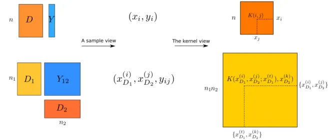
3.1.1 Pairwise kernel learning . . . 30
3.2 Multiple Kernel Learning. . . 31
3.2.1 MKL algorithms . . . 31
3.2.2 Overall comparison . . . 34
3.2.3 AlignF algorithm . . . 34
4 Tensor method for Multiple Kernel Learning 36 4.1 Factorized AlignF algorithm . . . 36
4.2 The optimal decomposition for the tensor of kernels . . . 38
5 Experiments 42 5.1 Data and experiment setup. . . 42
5.1.1 Artificially constructed datasets . . . 42
5.1.2 Real datasets . . . 44
5.1.3 Experiments setup . . . 45
5.2.1 Artificial constructed datasets . . . 47 5.2.2 Real-world datasets . . . 52 6 Discussion 59 7 Acknowledgement 60 References 61 A Appendix 65
List of Figures
1 Algorithms to be considered in this thesis. . . 1
2 Singular Vector Decomposition components . . . 4
3 Matrix factorization interpretation for an element . . . 5
4 Anorder-3 tensor . . . 6
5 Anorder-3 tensor with specific values. . . 6
6 A mode-1 fiber A(:, j, k), a mode-2 fiberA(i,:, k), and a mode-3 fiber A(i, j,:) . . . 7
7 A 3-order tensor fiber: A(:,1,1) . . . 7
8 A slice of theorder-3 tensor: A(:,:,2). . . 8
9 Rank-one third-order tensor . . . 8
10 The mode-1 unfolding example . . . 9
11 The mode-2 unfolding example . . . 9
12 The mode-3 unfolding example . . . 10
13 Tensor A of indices . . . 10
14 The CP decomposition for anorder-3 tensor . . . 18
15 The Tucker decomposition components for an order-3 tensor . . . 21
16 Tensor train decomposition and reconstruction for a specific element in a matrix . . . 25
17 The Tensor train decomposition and its reconstruction for a specific element in an order-3 tensor (cubic) . . . 25
18 Tensor train decomposition components for an order-4 tensor . . . 26
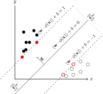
19 Components of the Support Vector Machine algorithm in two dimen-sional samples. . . 28
20 The comparison between kernel learning and pair-wise kernel learning 30 21 The framework of Factorization AlignF . . . 37
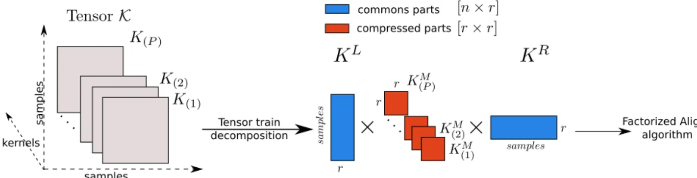
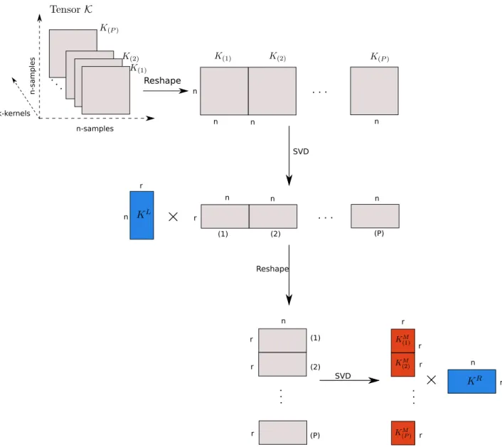
22 The Tensor Train algorithm decomposition steps for an order 3 tensor which is created by stacking kernels . . . 39
23 The graphical model of the generation process for a sample . . . 42
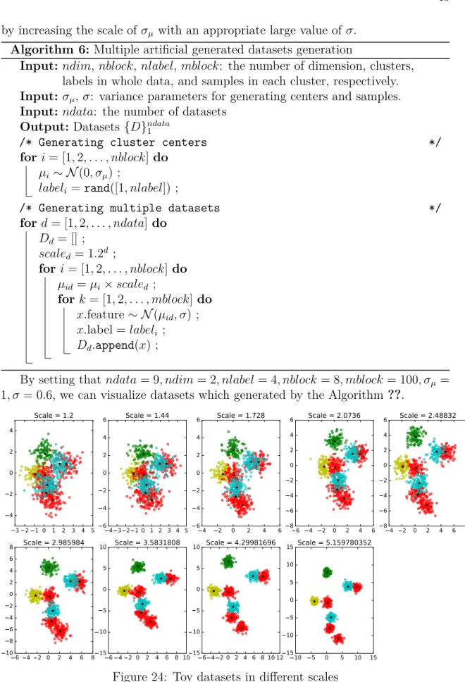
24 Toy datasets in different scales . . . 43
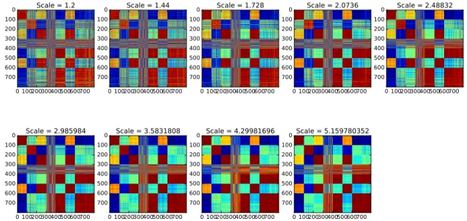
25 Linear kernels in different scale datasets . . . 44
26 Toy-data-1:Accuracy change in different datasets . . . 47
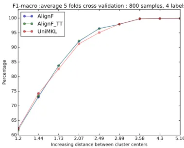
27 Toy-data-1:The macro-F1 change in different datasets . . . 48
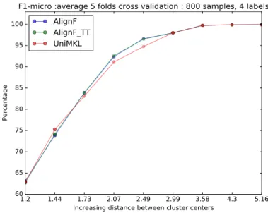
28 Toy-data-1:The micro-F1 change in different datasets . . . 49
29 Toy-data-2:Accuracy change in different datasets . . . 49
30 Toy-data-2:The macro-F1 change in different datasets . . . 50
31 Toy-data-2:The micro-F1 change in different datasets . . . 51
32 AlignF_TT performance in different low-rank numbers in Yeast data 54 33 AlignF_TT performance in different low-rank numbers in Emotions data . . . 54
34 AlignF_TT performance in different low-rank numbers in iaprtc12 data 55 35 AlignF_TT performance in different low-rank numbers inpsortPos data 55 36 AlignF_TT running time in different low-rank numbers in Emotions data . . . 56
37 AlignF_TT running time in different low-rank numbers in Enron data 57
38 AlignF_TT running time in different low-rank numbers in psortPos
data . . . 57
39 AlignF_TT running time in different low-rank numbers in psortNeg
data . . . 58
A1 AlignF_TT performance in different low-rank numbers in Enron data 65
A2 AlignF_TT performance in different low-rank numbers in Fingerprint
data . . . 66
A3 AlignF_TT performance in different low-rank numbers in Protein data 66
A4 AlignF_TT performance in different low-rank numbers in corel5k data 67
A5 AlignF_TT performance in different low-rank numbers in espgame data 67
A6 AlignF_TT performance in different low-rank numbers in iaprtc12 data 68
A7 AlignF_TT performance in different low-rank numbers inmirflickr data 68
A8 AlignF_TT performance in different low-rank numbers in pascal07 data 69
A9 AlignF_TT performance in different low-rank numbers inpsortPos data 69
A10 AlignF_TT performance in different low-rank numbers inpsortNeg data 70
1
Introduction
This thesis covers two major topics: the Tensor decomposition and its application in Multiple Kernel Learning. Related algorithms are described in the Figure 1.
Similarity based algorithms Multiple Kernel Learning Singular Value Decomposition Structured-risk based algorithms Centered kernel alignment (AlignF) CP
decomposition decompositionTucker
Tensor Train (TT) decomposition
Optimal Tensor Train decomposition for
multiple kernels
AlignF_TT (Factorized AlignF)
Figure 1: Algorithms to be considered in this thesis
This thesis first gives an overview of fundamental decomposition methods for matrices and tensors. In decomposing a matrix, Singular Value Decomposition (SVD) [1] algorithm represents a matrix as the weighted sum of rank-1 matrices or the multiplication of factor matrices. For a higher dimensional matrix or a tensor, decom-position algorithms are also derived from the SVD. The CANDECOMP/PARAFAC (CP) decomposition [2] takes the perspective of the weighted sum of rank-1 tensors while the Tucker decomposition [3] and Tensor Train decomposition [4] use SVD as the workhorse algorithm. Regarding the application, tensor decomposition methods also are employed in many fields: from linear algebra to machine learning, data mining, computer vision [5]. In Section 2, the primary objective is to derive solutions for these algorithms and relations, and for the potential applications.
Secondly, this study focuses on Multiple kernels learning [6], which has been studied mostly independently from tensor decomposition methods in the literature. The Multiple Kernel Learning (MKL) is a branch of the kernel learning method [7], where a set of kernels is available. The purpose of MKL is combining data from different sources and automatically selecting optimal kernels to improve the learning performance. Typically, these algorithms treat each kernel separately to find an optimal combination of them. To apply the tensor decomposition into these MKL
algorithms; this study focuses on two major MKL approaches based on the structured risk objectives [8] and kernel alignment algorithms [9]. Then Section 3 introduces the kernel learning framework, MKL algorithms and its development.
The fourth section describes two main findings of this study. One important finding is a novel algorithm for decomposing a tensor of kernels. Another interesting finding is a new centered kernel alignment algorithm which is based on the novel decomposition for the tensor of kernels. Then, Section 5 reports datasets and algorithm configurations to evaluate the performance of the proposed kernel alignment algorithm. Two sets of experiments are conducted on artificially constructed and real-world data sets. The first one manipulates in 18 artificially constructed datasets to evaluate the performance of kernel alignment algorithms under different data generation settings. The second experiment in 13 real-world datasets is conducted to compare the performance of algorithms in various kind of data including texts, images, and bioinformatics datasets.
1.1
Notation
• A vector containing all ones or zeros is denoted as1 or 0, respectively.
• x denotes a column vector and thus xT describes it in the row format.
• With (x, y, . . . , z) is the stacking of vectors to create a matrix in column order. The row stacking order as (xT;yT;. . .;zT) by using the semicolon.
• A full matrix is denoted in the mathbold type fonts: A.
• A general matrixA∈Rn×m is a stack of m vector as (x, y, . . . , z) where each x∈Rn.
• For a matrix A, Aij orA(i, j) is the element at row ith and column jth.
• The colon notation presents the row or column of a matrix. For example:
A(k,:) = [Ak1, Ak2, . . . , Akm] is kth row of a matrix.
• Σ is the diagonal matrix.
• σ is the singular value.
2
Tensor decomposition
2.1
Singular value decomposition
Finding the subspace that captures important properties of a dataset or the data-embedding configurations in a metric space is the crucial task in pattern recognition and machine learning [10]. By projecting data into this subspace and analysing the resulted data, many data-mining tasks can be solved; for example: dimensionality reduction, component interpretation, removing noise, and visualisation. To find this subspace, many well-known algorithms use Singular value decomposition (SVD) method [11] as the workhorse algorithm. For example, Principle Component Analysis aims to find the set of directions that explains most data variance and its solution corresponds to the SVD algorithm. Due to the importance of SVD in machine learning and data mining, this section describes its essential formulas and properties, along with some discussions relating to the tensor decomposition algorithms.
2.1.1 Singular value decomposition
Formally, the singular value decomposition of a matrix A ∈ Rn×m returns real
matrices U,V and a diagonal matrix with non-negative elements Σ which are satisfied:
A=UΣVT (1)
where
• U∈ Rn×n and V ∈Rm×m are orthogonal matrices and contain the left and
right singular vectors ofA as their columns, respectively.
• Σ∈Rn×m is the diagonal matrix that contains singular values σ
i in decreasing
order.
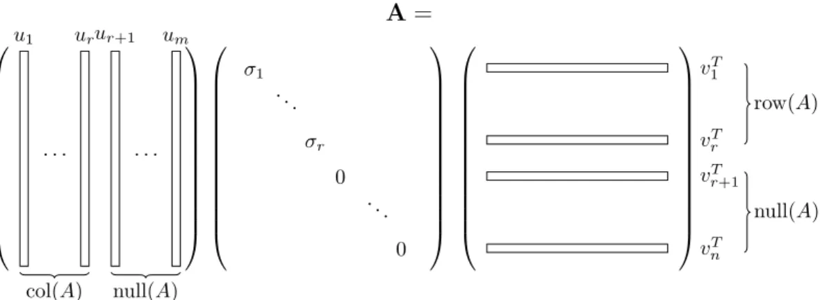
According to [11], the SVD can explicitly show the rank and the null space of a matrix. For the low-rank r ≤ min{m, n}, there are r vectors in the set of U =
{u1, u2, . . . , ur} spans the column space of A and the rest (m −r) vectors from U0 = {ur+1, ur+2, . . . , um} is the left null space ofA. The reason is when r >0 then UT0A =0 and a column in matrix A is the weighted linear combination from the vector in set U, then this set spans the column space of A. The same definition for the right singular matrix V.
SVD can equivalently written as:
A =
r
X
i=1
σiuiviT (2)
where each outer product uiviT returns a rank-one matrix, so A is the weighted
com-bination of rank-1 matrices. Pairs of eigenvectors associated with higher eigenvalues contains more information to reconstruct the original matrix.
In dimension reduction, the data ofn samples andm features is stored in a matrix
A = · · · · u1 urur+1 um col(A) null(A) σ1 . .. σr 0 . .. 0 vT 1 vT r vT r+1 vT n row(A) null(A)
Figure 2: Singular Vector Decomposition components
dimensional matrices with a high reconstruction accuracy. This property is proof in the Eckhart-Young theorem [12] which states that the SVD provides the best least square approximation for a matrix. In this case, the left singular matrixU∈Rn×k is
the solution and new feature values for each sample is the coordinate of this sample in the subspace that contains the largest amount of data variance. Particularly, if
k = 2, the dataset ofn points can be visualized in a 2 dimensional plan. This is due toU contains eigenvectors of the covariance matrix AAT of the data in A.
AAT = (UΣVT)(VΣUT) =UΣ2UT 2.1.2 Matrix factorization interpretation
The matrix factorization (MF) is the problem of approximating a matrix by the product of two matrices. The task is to find these matrices and typically they have a lower dimension than original data dimension.
A≈W×H (3)
where A ∈ Rn×m and W ∈ Rn×k, H ∈ Rk×m and k ≤ min(m, n). For each ith
columnA(:, i) in matrix A, we have:
A(:, i)≈W H(:, i) (4)
or each column of the original data is reconstructed by weighted combination of W
matrix with a corresponding column inH matrix.
In the other hand, W can be seen as thefeature matrix and His the coefficient
matrix. A column A(:, i) is the combination of newfeature matrix W with weights from corresponding column in the coefficient matrix H. In detail, the set of columns inW={w1, w2, . . . , wk}, then the data column reconstruction as follow:
A(:, i)≈
k
X
j=1
For a specific data element Aij, it is the weighted combination of row ith of W
and columnjth ofH.
Aij ≈W(i,:)×H(:, j) or Aij ≈W[i]×H[j]
where W[i] =W(i,:) ∈R1×k and H[j] =H(:, j)∈Rk×1, or having the same number
of dimension orlow-rank factors.
≈
×
Aij
W[i]
H[j]
Figure 3: Matrix factorization interpretation for an element
By this kind of representation, each original data element is reconstructed by the production of two vectors in the low-rank space. Then, with (n+m) indices for rows and columns, each index need a vector ∈ Rk to store its coefficients, the memory
complexity is O(k(m+n)).
In data mining applications, we can analyse properties of new data features through matrixW and the relations among original data features by using H [13]. For example, in text mining, the non-negative matrix factorization algorithms [14] are well developed for analyzing text data. The data is a document-term matrix where rows are documents and columns are the information of terms in each document. By finding a factorized representation, the matrix is decomposed into document-feature andfeature-term matrices, in which afeature stands for the lower dimensional approximation or data contents. Typically, thedocument-feature information is used for clustering documents or topic modeling.
Interestingly, the matrix factorization form can be achieved by using SVD. The SVD decomposition of matrix A=UΣVT, then the MF solution is:
W=Uk and H=ΣkVTk (5)
where Uk,Σk,Vk is the reduction of original matrix to contain only first largestk
eigenvalues and eigenvectors.
2.2
Tensors definition
Tensor is the multidimensional array of numerical values. Formally, anorder-d tensor is a d-dimensional array. For example, a scalar is an order-0 tensor, a vector and a matrix are anorder-1 and order-2 tensor, respectively. Additionally, the tensor formulation is a compact way to represent a multidimensional dataset. For example, a collection of documents that contains authors, terms, and publish dates can be seen as aorder-3 tensor. A colour image with 3 channels: R, G, B, can be seen as a tensor of [height× weight × colour]. Due to the tensor is the generalisation of the matrix,
the tensor decomposition is a generalisation of the low-rank decomposition for a matrix. This section will discuss the definition of tensor operators and decomposition algorithms which focus on CP decomposition (CANDECOMP/PARAFAC), Tucker decomposition [15], and Tensor Train decomposition [4].
Tensor notation The order of a tensor is in modes; for example, mode-1 of a matrix is its rows and columns are in mode-2. A general d-order real tensor is
A ∈Rn1×n2×···×nd and an element is A(i
1, i2, . . . , id) where the index range for mode kth is ik∈[1 : nk]. The colon notation “:” is used to indicate all elements in amode
or a specific index subset.
For example, the cube in Figure 4, a 3 dimensional array A ∈ Rn1×n2××n3 is
depicted as a cubic. Figure5shows the order-3 tensor: A ∈R3×4×2 in which mode-1
size is 3 and 4, 2 is for mode-2, mode-3, respectively.
1 : n 1 1 :n2 A 1:n 3
Figure 4: Anorder-3 tensor
13 14 15 16 17 18 19 20 21 22 23 24 1 2 3 4 5 6 7 8 9 10 11 12 A ∈R3×4×2
Figure 5: An order-3 tensor with specific values
Tensor parts: fiber and slice Parts of array or subarrays are made by fixing a subset of array indices. In a matrix or a mode-2 tensor, these parts are rows and columns and denoted as A(:, i) and A(j,:) for columni-th and row j-th, respectively. In a tensor, due to it has multi-dimensional indices, many possible indexing ways for using colon notation are available. This paragraph describe two special subarrays in tensors which are fiber and slice.
A fiber is a vector that is obtained by fixing all indices but one. For example, fibers are depicted in an order-3 tensor in Figure 6, 7.
A slice is a vector that is obtained by fixing all indices but two. For example, in Figure 8, a matrix is obtained when choosing all elements of two dimension and an index is fixed in the third dimension.
Figure 6: A mode-1 fiber A(:, j, k), a mode-2 fiber A(i,:, k), and a mode-3 fiber A(i, j,:) 13 14 15 16 17 18 19 20 21 22 23 24 1 2 3 4 5 6 7 8 9 10 11 12 A ∈R3×4×2
Figure 7: A 3-order tensor fiber: A(:,1,1)
Rank-one and diagonal tensor Analogically to the rank-one matrix, thed-order
rank-one tensor is formed by the outer product [11] ofdvectors. ForA ∈Rn1×n2×···×nd:
A =a(1)◦a(2)◦ · · · ◦a(d)
where a(k) is the k-th vector. Thus, an element A(i
1, i2, . . . , id) is the product of
corresponding elements in d vectors:
A(i1, i2, . . . , id) =a(1)(i1)a(2)(i2). . . a(d)(id)
For example, Figure9 visualizes the third-order rank-one tensor for A=a◦b◦c. A diagonal tensor A ∈Rn1×n2×···×nd that an element A(i
1, i2, . . . , id) is 1 if and
only ifi1 =i2 =· · ·=id.
Tensor norm The norm of a tensor A ∈ Rn1×n2×···×nd is the square root of the
sum of squares of all elements:
||A||F = v u u t n1 X i1 n2 X i2 · · · nd X id A(i1, i2, . . . , id)2
Matricization: mode-k unfolding In tensor computations, the typical step is tensorunfoldings or flattening which rearranges a tensor to a simpler form: a matrix, to utilize it well-foundation computations and discover patterns in the matrix from. According to [11], there are three main reasons to do that:
• Tensor operations can be reformulated as matrix operators through multiple unfolding steps.
13 14 15 16 17 18 19 20 21 22 23 24 1 2 3 4 5 6 7 8 9 10 11 12 A ∈R3×4×2
Figure 8: A slice of the order-3 tensor: A(:,:,2)
A =
a c
b
Figure 9: Rank-one third-order tensor
• An iterative tensor optimisation framework contains one or more unfolding steps.
• Hidden patterns of a tensor sometimes can be discovered through unfolding it into matrix forms.
There are several possible ways to assemble a tensor to a matrix. For example, we can rearrange a tensorA ∈ R3×4×2 in Figure5to a [12×2] matrix or a [4×6] matrix.
In this section, we discuss an important family of tensor unfolding which is the
mode-k unfolding. A(k) denotes themode-k unfolding of the tensorA ∈Rn1×n2×···×nd.
Formally, the size of A(k) is nk-by-(N/nk) where N =n1×n2× · · · ×nd and it is
the stacking of mode-k fibers in the column order. A tensor element (i1, i2, . . . , id)
maps to the matrix element (ik, j) by: j = 1 + nd X l=1;l6=k (il−1)Jl where Jl = nl Y l=1;l6=k nl (6) = 1 + (i1−1)n1+ (i2−1)n1n2+· · ·+ (id−1)(n1n2. . . nd)
Intuitively, this indexing system is analogous to the matrix indexing system by adding columns in other modes for flattening purpose. On the other hand, this step fixes one index system for a mode and stacking mode by mode for others. For the mode-k
unfolding, the index in the k position is preserved and all others are folded into one index. For example, the mode-1 matricization for a tensor in Figure5 is visualized in Figure 10. Following that, its mode-2 and mode-3 unfolding is in Figure 11, 12.
In detail, Figure 13 shows the unfolding example is in the indices format. Then, the mode-1 unfolding is:
A(1) = a111 a121 a131 a141 a112 a122 a132 a142 a211 a221 a231 a241 a212 a222 a232 a242 a311 a321 a331 a341 a312 a322 a332 a342
13 14 15 16 17 18 19 20 21 22 23 24 1 2 3 4 5 6 7 8 9 10 11 12 A ∈R3×4×2 1 2 3 4 13 14 15 16 5 6 7 8 17 18 19 20 9 10 11 12 21 22 23 24 A(1)=
Figure 10: The mode-1 unfolding example
1 5 9 13 17 21
2 6 10 14 18 22 3 7 11 15 19 23 4 8 12 16 20 24 A(2) =
Figure 11: The mode-2 unfolding example
A(2) = a111 a211 a311 a112 a212 a312 a121 a221 a321 a122 a222 a322 a131 a231 a331 a132 a232 a332 a141 a241 a341 a142 a242 a342 A(3) = " a111 a211 a311 a121 a221 a321 a131 a231 a331 . . .
a112 a212 a312 a122 a222 a322 a132 a232 a332 . . . #
Tensor product: mode-k product This section considers the tensor-matrix multiplication via the mode-k of a tensor. In general, the multiplication of two tensors can be derived as between matrices; this operator is called tensor contraction
which is clearly described in Chapter 12.4.9 of [11]. The mode-k or modal product is the special case and important family of the tensor contraction. This product operator needs a tensor, a matrix, and a specific mode. Formally, given a tensor
A ∈ Rn1×n2×···×nd and a matrix M ∈ Rmk×nk, the mode-k product is the matrix
multiplication of the mode-k unfoldingA(k) and M, and returns a tensor Y:
Y(k)=M× A(k) (7)
or according to [15], the shorted form of this equation is Y = A ×(k) M. The
configuration of these terms are the tensor A ∈ Rn1×n2×...nk−1×nk×nk+1×···×nd, the
matrix M ∈ Rmk×nk, the tensor Y ∈Rn1×n2×...nk−1×mk×nk+1×···×nd. In the
1 5 9 2 6 10 3 7 11 4 8 12 13 17 21 14 18 22 15 19 23 16 20 24 A(3)=
Figure 12: The mode-3 unfolding example
a112 a122 a132 a142 a212 a222 a232 a242 a312 a322 a332 a342 a111 a121 a131 a141 a211 a221 a231 a241 a311 a321 a331 a341 A ∈R3×4×2
Figure 13: Tensor A of indices
A(i1, . . . , ik−1,:, ik+1, . . . , id) for the mode-k product on the kth dimension.
Y(i1, . . . , ik−1,αk, ik+1, . . . , id) = nk X j=1 M(αk,j)A(i1, . . . , ik−1,j, ik+1, . . . , id) (8) with αk ∈[1 :mk]
For example, ifA ∈R3×4×2 is in Figure 13 andM∈R2×4, thenY
(2) =M× A(2): Y(2) = " a111 a211 a311 a112 a212 a312 a121 a221 a321 a122 a222 a322 # = " m11 m12 m13 m14 m21 m22 m23 m24 # × a111 a211 a311 a112 a212 a312 a121 a221 a321 a122 a222 a322 a131 a231 a331 a132 a232 a332 a141 a241 a341 a142 a242 a342
Intuitively, this multiplication replaces the content of the dimension k of A by weighted combination of this mode information with a matrix M. For the sequences of multiplications, when assuming component dimensions matches, the final result is independent the order [15].
A ×kM×hN=A ×hN×kM (h6=k) (9)
whereN∈Rzh×nh. Similarly, whenMis a vector or M∈R1×nk, themode-k product
between a tensor and a vector returns a d −1 dimensional tensor. It is easy to show that, the returned matrix Y ∈Rn1×n2×...nk−1×1×nk+1×···×nd and the equivalent
representation isY ∈ Rn1×n2×...nk−1×nk+1×···×nd .
Vec operator for a matrix The vector form is the common representation of a matrix and a tensor with some proper rearrangements. This vector representation or
vec operator allows to write matrices and tensors in the same form and thus faster the equation reduction step.
The operatorvecfor a matrix is the reshaping of a matrix X∈Rm×n to a vector of Rnm×1, by stacking columns of X . vec(X) = X(:,1) X(:,2) . . . X(:, n)
In detail, for a matrix X= "
a11 a12 a13 a21 a22 a23 # then vec(X) = a11 a21 a12 a22 a13 a23
Vec operator for a tensor is a generalisation of the matrix vectorization. This operator stacks columns from the last dimensional index as follow, for ad-dimensional
tensor A ∈Rn1×n2×···×nd: vec(A) = vec(A(1)) vec(A(2)) . . . vec(A(nd))
where A(k) is the (d−1)-dimensional tensor ∈Rn1×n2×···×nd−1, in which:
A(k)(i
1, i2, . . . , id−1) = A(i1, i2, . . . , id−1,k)
Note that,A(k) is different with A
(k) which is the mode-k matrix. A(k) is the copy
of original tensor when the last index id is fixed for a specific value k. For a d
dimensional tensor, this definition is recursive from A(k) of A, to (A(k0))(k) of A(k)
until fixing d−1 indexes to get a scalar, then go back to stack columns of higher order tensor columns. For example, the vec of anorder-3 tensor A2×3×2:
a112 a122 a132 a212 a222 a232 a111 a121 a131
is given by vec(A) = " vec(A(1)) vec(A(2)) # = " vec(A(:,:,1)) vec(A(:,:,2) # = a111 a211 a121 a221 a131 a231 a112 a212 a122 a222 a132 a232
Outer product The outer product◦is the product between two coordinate vectors. Formally, for vectors u ∈ Rm, v ∈ Rn then A = uvT = u◦v is a rank-1 matrix
∈Rm×n. For u= [u 1, u2, u3]T and v = [v1, v2]T: A=uvT = u1 u2 u3 h v1 v2 i = u1v1 u1v2 u2v1 u2v2 u3v1 u3v2 = v1 u1 u2 u3 , v2 u1 u2 u3 (10)
The outer product of more than 2 vectors returns a tensor. For example, the outer product of 3 vectors returns an rank-1 order-3 tensor, in which:
A =u◦v◦w and A(i, j, k) =u(i)v(j)w(k) (11) where u ∈ Rm, v ∈ Rn, w ∈ Rk and A ∈ Rm×n×k. For example, if u = [u
1, u2]T, v = [v1, v2]T, and w= [w1, w2]T, the u◦v◦w is:
u1v1w2 u1v2w2 u2v1w2 u2v2w2 u1v1w1 u1v2w1
u2v1w1 u2v2w1
Kronecker product In the case of scalar-matrix multiplication and doing this for many scalars in order to obtain a new block matrix, we need to use the Kronecker operator. Formally, for matricesB ∈Rm1×n1 andC∈Rm2×n2, the Kronecker product
D =B⊗C∈Rm1n1×m2n2 is a block matrix, in which a block at (i, j) is a matrix.
Thus,D is the m1-by-n1 block matrix whose (i, j) block is matrixb(i, j)Cof the size m2-by-n2. For example, if B∈R3×2 and C∈R2×2 then:
D =B⊗C= b11 b12 b21 b22 b31 b32 " c11 c12 c21 c22 # = b11C b12C b21C b22C b31C b32C =
b11c11 b11c12 b11c21 b11c22 b12c11 b12c12 b12c21 b12c22 b21c11 b21c12 b21c21 b21c22 b22c11 b22c12 b22c21 b22c22 b31c11 b31c12 b31c21 b31c22 b32c11 b32c12 b32c21 b32c22 (12)
The power of Kronecker product comes from its structure properties, fast practical algorithms, and connection between tensor and matrix computation [16]. Firstly, the vector form of matrices and tensors operators can be rewritten thanks to the Kronecker product. For matrices, Equation (10) is equivalent with:
A=u◦v = u1v1 u1v2 u2v1 u2v2 u3v1 u3v2 = v1 u1 u2 u3 ,v2 u1 u2 u3 ⇒vec(A) = v1u1 v1u2 v1u3 v2u1 v2u2 v2u3 = " v1 v2 # ⊗ u1 u2 u3 then vec(u◦v) = v⊗u
When the outer product returns a tensor, we do the same procedure for the example of Equation (11). For u= [u1, u2]T,v = [v1, v2]T, and w= [w1, w2]T:
A=u◦v◦w= " u1 u2 # ◦ " v1 v2 # ◦ " w1 w2 # ⇒vec(A) = u1v1w1 u2v1w1 u1v2w1 u2v2w1 u1v1w2 u2v1w2 u1v2w2 u2v2w2 = " w1 w2 # ⊗ u1v1 u2v1 u1v2 u2v2 = " w1 w2 # ⊗ " v1 v2 # ⊗ " u1 u2 # then vec(u◦v◦w) =w⊗v⊗u
As a tensor is a multi-dimension array, each mode-k matrix also can be described by the Kronecker product. By using the above example,A(1) is:
A(1) = " u1v1w1 u1v2w1 u1v1w2 u1v2w2 u2v1w1 u2v2w1 u2v1w2 u2v2w2 # = " u1 u2 # ⊗hv1w1 v2w1 v1w2 v2w2 i
= " u1 u2 # ⊗ v1w1 v2w1 v1w2 v2w2 T = " u1 u2 # ⊗ " w1 w2 # ⊗ " v1 v2 #!T then A(1) =u⊗(w⊗v)T
These rules describe the Kronecker representation among tensors and matrices:
A =u(1)◦u(2)◦. . . u(d) ∈Rn1×n2×···×nd then vec(A) =u(d)⊗u(d−1)· · · ⊗u(2)⊗u(1) (13) A(k)=u(k)⊗ u(d)⊗. . . u(k+1)⊗u(k−1)· · · ⊗u(2)⊗u(1)T (14) A sequence of matrix-matrix multiplications can be represented in the Kronecker product with vec operator. For matrices: Y ∈ Rm2×m1, C∈Rm2×n2, X ∈ Rn2×n1,
and B∈Rm1×n1
Y=CXBT ⇔ vec(Y) = (B⊗C)vec(X) (15)
A very clear example for Equation (15) is in Chapter 1.3.5 of [11]. From the Equation (12), we can see that the structure property of resulted matrix from B⊗C
is dependent on the structure of B. Then if B has a band structure (diagonal, tridiagonal, lower/upper triangular ) then the B⊗Cretains the same structure as
B.
From [16], some notable properties of the Kronecker product is: (B⊗C)T = BT ⊗CT
(B⊗C)(D⊗F) = (BD)⊗(CF) (16)
(B⊗C)⊗D = B⊗(C⊗D) (B⊗C)† = B†⊗C†
Hadamard product The Hadamard product definition is quite straight-forward, it is the elementwise product for matrices of similar size. Formally, the Hadamard product between two matrices B,C∈Rm×n is:
A=B∗C and A∈Rm×n
A(i, j) =B(i, j)C(i, j)
Shortly, an element ofA is the multiplication of 2 corresponding elements from B
Khatri-Rao product is the special case of Kronecker product when two matrices contain the same number of columns. Formally, the Khatri-Rao product between two matricesB ∈Rm1×n and C∈Rm2×n is:
A =BC and A∈Rm1m2×n
This product is the columwise product where matched column are multiplied by the Kronecker product. For example, the separation of matricesB,C into columns are:
B = [b1 |b2 | . . . |bn] and C= [c1 |c2 | . . . |cn]
wherencolumns are available and eachbi ∈Rm1×1 andci ∈Rm2×1. We can represent
the Khatri-Rao product to get A as follow:
A= [b1⊗c1 |b2⊗c2 | . . . |bn⊗cn]
where ai = bi⊗ci return a column vector of size m1-by-m2 and the number columns
of A remainsn.
According to [15], the properties of Khatri-Rao product:
ABC = (AB)C=A(BC)
(AB)T(AB) = ATA∗BTB (17)
(AB)† = ((ATA)∗(BTB))†(AB)T
Multilinear product is the product among one tensor and many matrices where giving a tensor A ∈Rn1×n2×···×nd, a tensor S ∈Rr1×r2×···×rd, and d matricesM
k ∈ Rnd×rd. Then, the multilinear product among tensor S and multiple matrices M
creates a tensor A: A=S ×1M1×2M2· · · ×dMd (18) A(i1, i2, . . . , id) = r1 X j1 r2 X j2 · · · rd X jd S(j1, j2, . . . , jd)M1(i1, j1)M2(i2, j2). . .Md(id, jd) or equivalent with vec(A) = (Md⊗Md−1 ⊗ · · · ⊗M1)vec(S) (19)
regarding to the mode-k matrix of A
A(k)=Mk· S(k)·(Md⊗Md−1⊗. . .Mk+1⊗Mk−1· · · ⊗M1)T (20)
In order to make these definitions clear, we will cover an example for order-2 tensor and make the generalisation:
In the matrices case, the multilinear product according to these matrices: A ∈
Rn1×n2, S∈Rr1×r2,M
1 ∈Rn1×r1, and M2 ∈Rn2×r2. Then A =S×1M1×2M2 =M1SMT2
For example, with S,M1,M2 ∈R2×2, then A∈R2×2, in which: M1 = " a11 a12 a21 a22 # ; S= " s11 s12 s21 s22 # ; M2 = " b11 b12 b21 b22 # ; MT2 = " b11 b21 b12 b22 # then " A(1,1) A(1,2) A(2,1) A(2,2) # = (a11s11+a12s21)b11 (a11s11+a12s21)b21
+(a11s12+a12s22)b12 +(a11s12+a12s22)b22
(a21s11+a22s21)b11 (a21s11+a22s21)b21
+(a21s12+a22s22)b12 +(a21s12+a22s22)b22
= " a11s11b11+a12s21b11+a11s12b12+a12s22b12 a11s11b21+a12s21b21+a11s12b22+a12s22b22 a21s11b11+a22s21b11+a21s12b12+a22s22b12 a21s11b21+a22s21b21+a21s12b22+a22s22b22 # then vec(A) =
a11b11+a12b11+a11b12+a12b12 a21b11+a22b11+a21b12+a22b12 a11b21+a12b21+a11b22+a12b22 a21b21+a22b21+a21b22+a22b22
× s11 s21 s12 s22 = " b11 b12 b21 b22 # ⊗ " a11 a12 a21 a22 #! × s11 s21 s12 s22 = (M2⊗M1)vec(S)
From these equations we can infer these facts:
A(i, j) =X r1 X r2 S(r1, r2)M1(i, r1)M2(j, r2) then A = X r1 X r2 S(r1, r2) (M1(:, r1)◦M2(:, r2)) = X r1 X r2 S(r1, r2) (M2(:, r2)⊗M1(:, r1))
or vec(A) = (M2⊗M1)vec(S) as in above example. From this point of view, we
can make the generalisation to higher order tensor to get the equivalence between Equation (18) and (19).
For the mode-k matrix of a multilinear product, we utilize the property of mode-k
product that:
A = S ×1M1 ×2M2· · · ×dMd
= S ×kMk×1M1· · · ×k−1Mk−1×k+1Mk+1· · · ×dMd
then
2.2.1 SVD revisited
A Singular Value Decomposition for a matrix is equivalent to a multilinear product of matrices in above example. The correspondence is evident by substituting U=M1, Σ=S, V=M2, andS is diagonal. Then, there are 2 ways of expression for SVD
from multilinear product perspective: A=UΣVT: A(i, j) =X r1 X r2 Σ(r1, r2)U(i, r1)V(j, r2) and A = X r1 X r2 Σ(r1, r2) (U(:, r1)◦V(:, r2)) = X r λr(U(:, r)◦V(:, r))
asS is a diagonal matrix and λr = Σ(r, r).
The first direction describes the actual result from multilinear product and the latter can be seen as the weighted sum of rank-1 matrices. These results are matched with our pre-knowledge about SVD and its derivations.
Then an order-2 tensor has 2 ways of description in order to reconstruct it from other matrices. In order to generalize these properties for higher order tensor, main ideas are still relied on these observation of SVD representation.
There are two principal algorithms to decompose a tensor: CP(CANDECOMP/PARAFAC) and Tucker. The CP decomposition produces a weighted sum of rank-1 tensors and
the Tucker decomposition is the multilinear product for high order tensors. In the following sections, we will discuss these decomposition algorithms in detail along with a new way of decomposing a tensor: Tensor-Train algorithm.
2.3
CP decomposition
The CP decomposition is introduced as many names from different publications: CANDECOMP [17], PARAFAC [18], and CP in [2]. Formally, given a tensor:
A ∈Rn1×n2×···×nd, it finds a tensor approximation ˆX that:
min ˆ X ||A −X ||ˆ F where ˆ X = r X i=1 λi a(1)i ◦a (2) i · · · ◦a (k) i · · · ◦a (d) i (22) ˆ
X is the nearest approximation of the tensor A in terms of weighted sum of rank-1 tensors. The vector componenta(k)
r ∈Rnk
×1 stands for the contribution of dimension kth in the rank rth. This equivalent formula is derived from the property of the multilinear product: ˆ X = r X i=1 λi M(1)(:, i)◦M(2)(:, i)· · · ◦M(d)(:, i)
where M(k) ∈Rnk×r. Intuitively, each modekth is compressed into a matrixn k-by-r
instead ofnk-by-(n1×n2· · · ×nk−1×nk+1. . . nd) from the tensor unfolding property.
For example, in anorder-3 tensor, the nearest approximation from CP decomposition is showed in the Figure 14. in which:
ˆ X = a1 λ1 c1 b1 + λ2 a2 c2 b2 +. . .
Figure 14: The CP decomposition for an order-3 tensor
ˆ X = r X i=1 λi ai◦bi◦ci (23) where A ∈Rn1×n2×n3 and a i ∈Rn1×1, bi ∈Rn2×1,ci ∈Rn3×1 2.3.1 Tensor rank
Firstly, we recall the matrix rank that is the number of dimension of the vector space which spans its columns. However, the tensor rank definition is quite different and not a generalisation of the matrix rank.
The rank of a tensor A is denoted asrank(A) and it is the smallest number of required rank-one tensors to exactly reconstructA as in Equation (22). For example, a tensorA ∈Rn1×n2×···×nd is called as a rank-R tensor if:
A = R X i=1 λi a (1) i ◦a (2) i · · · ◦a (k) i · · · ◦a (d) i (24)
Following the elaborated article [15] and book [11], we will discuss some complication of tensor rank.
• Determining the rank of a tensor is a NP-hard problem.
• There is more than one rank that is available for a tensor. For example from [15], for a [2×2×2] tensor, authors determine that 79% of the space is filled by rank-2 and the rest 21% for rank-3.
• The maximum rank is the largest rank can be obtained for a tensor. It is not straight forward as max{n1, n2, . . . , nd}.
• The typical rank is any rank-r that fit the Equation (24) or any rank that occurs with positive probability.
• A typical rank for an order-3 tensor are already calculated. For example: a tensor 2×2×2 has a typical rank is {2,3} and this number is {3,4}, {5,6}
• For a general order-3 tensor: A ∈Rn1×n2×n3, the upper bound for its rank is rank(A)≤min(n1n2, n2n3, n1n3).
2.3.2 The algorithm
In this section, we focus on the CP decomposition algorithm based on Alternating Least Square procedure which is proposed in [17], [18]. In order to make the algorithm to be understandable, we firstly find the solution for an order-3 tensor and derive the final algorithm for a general order-d tensor.
Given a tensor: A ∈ Rn1×n2×n3, the objective is finding an approximation of
tensor ˆX that: min ˆ X ||A −X ||ˆ F (25) ˆ X = r X i=1 λi M(1)(:, i)◦M(2)(:, i)◦M(3)(:, i)
where M(k) ∈ Rnk×r. This objective function is represented by unfolding its into mode-k matrices:
||A −X ||ˆ F =||A(1)−Xˆ(1)||F =||A(2)−Xˆ(2)||F =||A(3)−Xˆ(3)||F
These objective functions are solved iteratively. Firstly, in the mode-k unfolding, we need to find the corresponding CP approximation of this mode in the matrix form. As the CP decomposition objective function (25) is in the multilinear product form where the diagonal tensor S including λ, we can rewrite that:
ˆ X(1) = r X i=1 λi M(1)(:, i)· M(3)(:, i)⊗M(2)(:, i)T = M(1)·diag(λ)·M(3) M(2)T where diag(λ) = λ1 . . . . . . . . . . . . λd
is the diagonal matrix contains all mixing coefficients.
The term of (M(3)(:, i)⊗M(2)(:, i)) is the Kronecker product of vectors in M(3) and M(2) in the same column index. Thus, it is the column-wise Kronecker product or
equivalent with the Khatri-Rao product between two matrices of the same number of columns.
Equivalently, we obtain the derivation for ˆX(2) and ˆX(3):
ˆ X(2) = M(2)·diag(λ)· M(3) M(1)T ˆ X(3) = M(3)·diag(λ)· M(2) M(1)T
find {diag(λ),M(1),M(2),M(3)} so that these quantities to be minimized: ||A(1)−M(1)·diag(λ)· M(3) M(2)T ||F ||A(2)−M(2)·diag(λ)· M(3) M(1)T ||F ||A(3)−M(3)·diag(λ)· M(2) M(1)T ||F
The Alternating Least Square (ALS) strategy is used by fixing all variables except one and solve the corresponding objective function. For example, when fixingM(3),M(2),
we need to find the minimize of this function:
||A(1)−M˜(1)·
M(3) M(2)T ||F
where ˜M(1) =M(1)·diag(λ). Then the least squares solution is:
˜
M(1) =A(1)
M(3) M(2)T
†
As the above equation need the inversion of a big matrix ∈Rn3n2×r, nevertheless we
can calculate this quantity without doing this inversion thanks to the properties of Khatri-Rao product:
˜
M(1) =A(1)
M(3) M(2) (M(3))TM(3)∗(M(2))TM(2)† (26) After getting the solution for ˜M(1), we can get the solution forλ
j andM(1) after this
normalization:
λj = ||M˜(1)(:, j)||2 (27)
M(1)(:, j) = ||M˜(1)(:, j)||/λj
Finally, we can make a generalisation algorithm for a d-order tensor based on Equations (26) and (27).
Algorithm 1: The CP decomposition algorithm based on Alternating Least Square procedure
Data: A d-order tensor A ∈Rn1×n2×···×nd Input: The intended rank r
Output: diag(λ), M(1),M(2), . . . ,M(d)
Initialize M(k) ∈Rnk×r randomly ; while !stop-condition do
for k = [1,2, . . . , d]do
/* least squares solution (26) */
V =M(d)TM(d)∗. . .M(k+1)TM(k+1)∗M(d)TM(d)· · · ∗M(1)TM(1); ˜ M(k) =A (k) M(d). . .M(k+1)M(k−1)· · · M(1)V†;
/* update the solution as Equation (27) */
for j = [1,2, . . . , r] do
Updateλj ;
2.4
Tucker decomposition
The Tucker decomposition is invented by Tucker [19], [3] and also has many names, the most related under the name Higher Order SVD (HOSVD) [20]. The multilinear product description is still the central matter. While the CP decomposition is based on the diagonal tensor S, the Tucker decomposition uses a full one. Formally, given a tensor A ∈ Rn1×n2×···×nd, a tensor S ∈ Rr1×r2×···×rd, and d matrices in which Mk ∈ Rnd×rd. The Tucker decomposition objective function is finding a nearest
tensor ˆX which is in the form of multilinear product: min ˆ X ||A −X ||ˆ F (28) ˆ X =S ×1M1 ×2M2· · · ×dMd
For example, for anorder-3 tensorA ∈ Rn1×n2×n3, the decomposition components
are illustrated in Figure 15.
ˆ X = S M2 M3 M1
Figure 15: The Tucker decomposition components for an order-3 tensor Due to the tensor S not being diagonal, we need to take care about the rank of each mode: {r1, r2, . . . , rd}. We need to define the specific value forri or find an
efficient value for it. The HOSVD is based on the SVD definition and ranks for each
mode-k matrix while the Tucker decomposition can achieve a higher compression by user-defined ranks.
2.4.1 The n-rank and multilinear rank
In order to distinguish the HOSVD and Tucker decomposition, we need to define notation for ranks of tensor modes. There are two common definitions:
• In [15], then-rank for a tensor orrankn(A) is the rank of the matrix based on mode-n unfolding: A(n). It is the column rank of matrix A(n).
• In [11], the multilinear rank orrank∗(A) contains all n-rank of all modes. rank∗(A) = {rank1(A),rank2(A), . . . ,rankd(A)}
2.4.2 The Higher Order SVD (HOSVD)
We can find an exact solution for Equation (28) whenrk =rankk(A) for all modes.
for each mode. Given a tensor A, the SVD decomposition for each mode is:
A(k) =UkΣkVTk
Recall that A(k) is the matrix of nk-by-(n1n2. . . nk−1nk+1. . . nd), thus the rank rankk(A)≤min(nk, n1n2. . . nk−1nk+1. . . nd) and Uk expands the column space of
A(k). According to [20], its HOSVD is given by:
A = S ×1U1×2U2· · · ×dUd (29)
S = A ×1UT1 ×2 UT2 · · · ×dUTd
where UT k = U
†
k as the matrix Uk is columns orthogonal. Noted that the tensorS is
called core tensor.
Algorithm 2: The HOSVD decomposition algorithm
Data: A d-order tensor A ∈Rn1×n2×···×nd Input:
Output: S, M(1),M(2), . . . ,M(d)
Initialize M(k) ∈Rnk×r randomly ; for k= [1,2, . . . , d]do
/* SVD decomposition for each mode */
A(k) =UkΣkVTk; M(k) =U
k;
/* update the core tensor */
S =A ×1UT1 ×2UT2 · · · ×dUTd ;
Intuitively, the algorithm independently decomposes the tensor in each mode to capture the mode-variance. Then thecore tensor stores the interaction information among separated modes to reconstruct the tensor.
2.4.3 Tucker decomposition algorithm
In the case ofrk <rankk(A) in at least one mode or if one is aiming to achieve lower rk, the HOSVD algorithm can be applied by taking less columns for the left singular
matrix Uk. However, thistruncated HOSVD does not give the optimal solution for
the Tucker approximation objective function (28).
In order to derive a solution, firstly we analyse the Tucker optimization problem in an order-3 tensor and make a generalisation latter. From vectorization properties of the multilinear product, the equivalent objective function of (28) is
||A −X ||ˆ F =||vec(A)−
M(3)⊗M(2)⊗M(1)vec(S)||2
As M(3)⊗M(2)⊗M(1) is column orthogonal so the solution for core tensor is: vec(S) =M(3)⊗M(2)⊗M(1)T vec(A)
We get the new objective function by putting it back to the objective function: min
M ||vec(A)−MM T
where M=M(3)⊗M(2)⊗M(1). Moreover, we can shorten it more by:
||vec(A)−MMTvec(A)||2
= ||vec(A)||2−2hvec(A),MMTvec(A)i+||MMTvec(A)||2
= ||vec(A)||2−2vec(A)TMMTvec(A) +||MTvec(A)||2
= ||vec(A)||2− ||MTvec(A)||2
where the last terms are equivalent as MTM =I as M is column orthogonal. As the term||vec(A)||2 is a constant then the final objective function is to maximize
that quantity: ||M(3)T ⊗M(2)T ⊗M(1)Tvec(A)||2 = ||M(1)T · A (1)·(M(3)⊗M(2))||F ||M(2)T · A (2)·(M(3)⊗M(1))||F ||M(3)T · A (3)·(M(2)⊗M(1))||F
At this point, we can apply the Alternating Least Squares to solve objective functions in modes. In each mode, it leads to another optimization problem that given a matrix
A find the best projection Q: min
Q ||Q
TA||
F s.t QTQ=I
For example, in solving minM(1)||M(1)T · A(1) ·(M(3) ⊗M(2))||F, the A matrix is
corresponding to A(1)·(M(3)⊗M(2))
and Q is the matrix M(1).
Fortunately, this problem solution comes from the decomposition of A= USVT
as ||QTA||F =||QTUSVT||F =||QTUS||F = r X i=1 λi||QTU(:, i)||2
Then the solution for this nonnegative maximization problem is the top ˆreigen-vectors of the left singular matrixU. Then the final algorithm follows:
Algorithm 3: The ALS Tucker decomposition algorithm
Data: A d-order tensor A ∈Rn1×n2×···×nd Input: Input ranks{r1, r2, . . . , rd}
Output: S, M(1),M(2), . . . ,M(d)
Initialize M(k) ∈Rnk×r randomly or fromtruncated HOSVD; for k= [1,2, . . . , d]do Vk=A (k)·(M(d)⊗. . .M(k+1)⊗M(k−1)· · · ⊗M(1)) ; /* SVD decomposition */ Vk=UkΣkVTk; M(k) =U k(:,1 :rk);
/* update the core tensor */
2.5
Tensor train decomposition
2.5.1 Analysis and definitionWe already discuss about two fundamental tensor decomposition algorithms: CP and Tucker decomposition. However, these algorithms are not optimal in terms of efficiency and stability. In the ideal case, if we have a d-order tensor and each dimension contains n elements, then we need nd numbers to store it. In the CP
decomposition, the approximation from R rank-1 tensors needs Rdn parameters and it is a quite small number in comparison with nd parameters. However, it is a NP-hard problem in determiningR and the CP algorithm is an ill-posedness problem [21]. On the other hand, the Tucker decomposition is optimal but it suffers a high complexity of O(Rd+dnR) parameters and thus remaining in the bottle neck of the dimensionality curse.
Recently, the Tensor Train decomposition [4] has emerged as an efficient decom-position algorithm that is stable and low complexity. It is a special case of thetensor network [22] where a higher order tensor is approximated by many low-order tensors and contraction operators (reshape and multilinear products). Thisnetwork includes nodes as low-order tensors and edges operates the contraction. Formally, given a tensor A ∈Rn1×n2×···×nd where each dimensionkth the indexing isi
k ∈[1,2, . . . , nk],
the Tensor Train decomposition of A is the multiplication of low-rank matrices Gi in
specific indicies for a specific element A(i1, i2, . . . , id):
A(i1, i2, . . . , id) =G1[i1]G2[i2]. . .Gd[id] (30)
where Gk is a 3-order tensor of rk−1 ×nk×rk and Gk[ik] is a matrix of rk−1×rk
with rk is the low-rank. In addition, the boundary conditions that r0 =rd = 1 in
order to get A(i1, i2, . . . , id) is a scalar. On the other hand, the TT can be seen as a
tensor factorization method, when a tensor can be described by the multiplication of factors, each factor is a low-order tensor according to one index in a dimension.
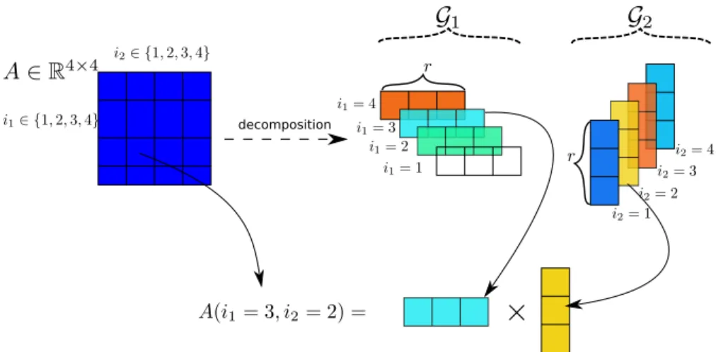
TT decomposition for a matrix Firstly, a matrix is also an order-2 tensor, so the TT decomposition is equivalent to the matrix factorization. In Figure16, a 4-by-4 matrix A is decomposed into 2 smaller matrices G1,G2 (order-2 tensors). In each Gk,
there are 4 vectors according to 4 indices that make the low-rank approximation for each specific dimension index of A. To reconstruct an element A(3,2), the 3rd component of G1 and the 2nd component of G2 are taken to do the multiplication.
Noted that, in this case of an order-2 tensor then bothGk are satisfy the boundary
conditions that r0 =r3 = 1 then G1 is r0×n1×r1 or 1×n1 ×r1 and the same for
G2 of r1×n2×1
TT decomposition for an order-3 tensor Similarly, for an order-3 tensor we need to add an additional tensorG2 in decomposition components which stands for the
second dimension. Figure 17shows the TT decomposition for a tensorA ∈ R4×2×3:
decomposition
Figure 16: Tensor train decomposition and reconstruction for a specific element in a matrix
• G2 ∈Rr1×2×r2
• G3 ∈Rr2×3×1
decomposition
Figure 17: The Tensor train decomposition and its reconstruction for a specific element in an order-3 tensor (cubic)
If r1 = 4 and r2 = 2, then we have an exact TT decomposition for A and thus it
is an approximation when r1 <4 and r2 <2. In this case, each G2[i2] is a matrix
of r1×r2 for a specific index i2 in the second dimension. Intuitively, this matrix
captures interactions of all indices in the first and third dimension that go through a specific index in 2nd dimension. Finally, in order to reconstruct an element from a tensor, we take the multiplication of corresponding low-order tensor elements based on its indices.
TT decomposition for a order-4 tensor For a tensor that its order is higher than 3, the visualization comes to thetrain style. For an order-4 tensorA ∈Rn1×n2×n3×n4,
the TT decomposition train in Figure 18is: • G1 ∈R1×n1×r1 • G2 ∈Rr1×n2×r2 • G3 ∈Rr2×n3×r3 • G4 ∈Rr3×n4×1 G1 k1 G2 k2 G3 k3 G4
Figure 18: Tensor train decomposition components for an order-4 tensor For each element of