FACTORS AFFECTING THE
PERFORMANCE OF TRAINABLE
MODELS FOR SOFTWARE DEFECT
PREDICTION
by
DAVID HUTCHINSON BOWES
Submitted to the University of Hertfordshire in partial fulfilment of the requirements of the degree of
DOCTOR OF PHILOSOPHY
School of Computer Sciences University of Hertfordshire
Acknowledgements
My first and foremost acknowledgement goes to Tracy Hall. It is while working with Tracy that I have learnt the dogma: the need for RIGOUR and the concept of FOCUS; how can I do better. Rigour means that every word has to be justified and consistent1. Focus means that this dissertation is not the original 500 pages. How can I do better? means that although this dissertation has ended, the work has not. My second acknowledgement goes to my other supervisors, Neil Davey and Bruce Christianson. It has bean a pleasure working with them and learning the different ways of doing and thinking about research. My third acknowledgement goes to my parents who provided a stimulating and thought provoking en-vironment in my formative years which I constantly reflect on while bringing up my own son.
My fourth acknowledgement goes to Kath Walley, my A’level physics teacher who introduced me to the problem of measurement error.
My fifth acknowledgement goes to my examiners (Prof. Barbara Kitchenham, Prof. Mark Harman and Dr. Nathan Baddoo) who have rigorously checked every equation and detail which makes this final version better than the last.
My penultimate acknowledgement goes to Jenny Jeffery for her proof reading of this dissertation and for the professionalism that she taught me while sharing an office and managing a Sixth Form in a large Secondary School.
My last acknowledgement is to the other colleagues who I have worked with while teaching and re-searching. Their contribution has been inspirational and usually good fun.
Finally, when my Dad died he left me his collection of books. Included in his collection was a handwrit-ten book which contained a dissertation of all the answers to the questions I had asked him, but he had never answered. I had always thought it strange that he would not answer some questions even though he was more than capable of answering them. I have come to the conclusion that he thought it better for me to work out the answers myself rather than being fed someone else’s answer. It is probably his dogma, that has made me continue asking why. At the end of his dissertation he included a glossary of all of his favourite sayings which as a child I had heard him repeat many times. However, at the start of the list was one saying I had never heard him say :
“If you have time to waste, don’t waste it on those who are busy!” D.C.Bowes.
iii
ABSTRACT
Context.Reports suggest that defects in code cost the US in excess of $50billion per year to put right.
Defect Prediction is an important part of Software Engineering. It allows developers to prioritise the code that needs to be inspected when trying to reduce the number of defects in code. A small change in the number of defects found will have a significant impact on the cost of producing software.
Aims. The aim of this dissertation is to investigate the factors which affect the performance of
defect prediction models. Identifying the causes of variation in the way that variables are computed should help to improve the precision of defect prediction models and hence improve the cost eff ective-ness of defect prediction.
Methods. This dissertation is by published work. The first three papers examine variation in the
independent variables (code metrics) and the dependent variable (number/location of defects). The fourth and fifth papers investigate the effect that different learners and datasets have on the predictive performance of defect prediction models. The final paper investigates the reported use of different machine learning approaches in studies published between 2000 and 2010.
Results. The first and second papers show that independent variables are sensitive to the
mea-surement protocol used, this suggests that the way data is collected affects the performance of defect prediction. The third paper shows that dependent variable data may be untrustworthy as there is no reliable method for labelling a unit of code as defective or not. The fourth and fifth papers show that the dataset and learner used when producing defect prediction models have an effect on the performance of the models. The final paper shows that the approaches used by researchers to build defect prediction models is variable, with good practices being ignored in many papers.
Conclusions. The measurement protocols for independent and dependent variables used for
de-fect prediction need to be clearly described so that results can be compared like with like. It is possible that the predictive results of one research group have a higher performance value than another research group because of the way that they calculated the metrics rather than the method of building the model used to predict the defect prone modules. The machine learning approaches used by researchers need to be clearly reported in order to be able to improve the quality of defect prediction studies and allow a larger corpus of reliable results to be gathered.
Contents
1 Introduction 1
1.1 Aim . . . 1
1.2 Introduction . . . 2
1.3 Thesis and Research Questions . . . 3
1.4 Contributions to Knowledge . . . 3
1.5 Structure of this Dissertation . . . 5
2 A Summary of Defect Prediction 7 2.1 Introduction . . . 7
2.2 What is a Defect? . . . 7
2.2.1 What is the Purpose of Defect Prediction? . . . 7
2.2.2 What is Defect Prediction? . . . 8
2.2.3 Code Defects . . . 8
2.3 Variables Used in Defect Prediction Studies . . . 10
2.3.1 Independent Variables . . . 11
2.3.2 Dependent Variables . . . 11
2.4 Modelling Techniques . . . 11
2.4.1 Continuous Techniques . . . 12
2.4.2 Categorical Techniques . . . 14
2.5 Data Quality and Data Cleaning . . . 20
2.6 Model Building Approaches . . . 20
2.6.1 Building Generalisable Models. . . 20
2.6.2 Testing the Generalisability of Models . . . 21
2.7 Issues of Model Building Specific to Machine Learning . . . 21
2.7.1 Dealing with Datasets which are Unbalanced . . . 22
2.7.2 Machine Learning Model Optimisation . . . 22
2.7.3 Model Tuning. . . 23
2.7.4 Reordering the Training Data . . . 23
2.8 Measuring the Performance of a Model . . . 25
2.8.1 Measuring the Performance of Categorical Prediction Models . . . 25
2.9 Summary of Techniques . . . 28
2.10 Conclusion . . . 28
3 Contribution of Papers 31 3.1 Introduction . . . 31
3.2 RQ1: Does the measurement protocol for the independent variables affect the metric values produced? . . . 31
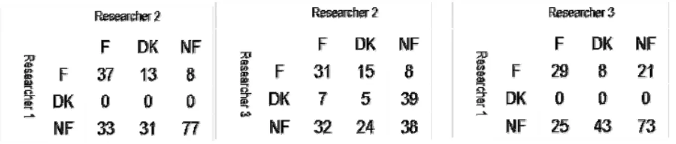
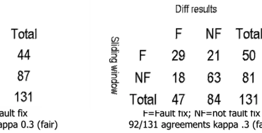
3.3 RQ2: Is there an effective method for deriving the dependent variables for defect pre-diction? . . . 33
3.4 RQ3: Which factors (dataset, learner) affect the performance of defect prediction studies? 34 3.5 RQ4: Are the results of machine learning studies reliable/trustworthy? . . . 35
vi Contents
4 Papers 39
4.1 Paper 1: Calibrating program slicing metrics for practical use. . . 41
4.2 Paper 2: The Inconsistent Measurement of Message Chains. . . 45
4.3 Paper 3: Evaluating Three Approaches to Extracting Fault Data from Software Change Repositories. . . 55
4.4 Paper 4: A Systematic Literature Review on Fault Prediction Performance in Software Engineering.. . . 67
4.4.1 Corrigendum . . . 67
4.5 Paper 5: Comparing the performance of fault prediction models which report multiple performance measures: recomputing the confusion matrix. . . 99
4.5.1 Corrigenda . . . 99
4.6 Paper 6: The State of Machine Learning Methodology in Software Fault Prediction. . . . 111
5 Conclusion 119 5.1 Reflection on the Research Questions . . . 119
5.2 Main Findings. . . 121
5.2.1 Analysis . . . 122
5.3 Future Work . . . 123
5.3.1 Statistical Analysis of the Impact of Different Measurement Protocols on being able to Predict Defects . . . 124
5.3.2 Measurement Protocols. . . 124
5.3.3 Reporting Protocols . . . 124
5.3.4 The Need for Replication Studies . . . 124
5.3.5 Ensuring Consistency in Machine Learning Approaches . . . 125
5.3.6 Building Repositories of Comparable Data . . . 125
5.3.7 Why not What! . . . 125
5.4 Final Remarks. . . 126
References 127 Appendices 134 A Reviewers’ Comments for [Bowes et al. 2012b] 135 B Additional Papers 137 B.1 Cohesion metrics: the empirical contradiction.. . . 137
B.2 Using program slicing data to predict code faults. . . 145
B.3 Program slicing-based cohesion measurement: the challenges of replicating studies us-ing metrics. . . 163
B.4 Developing fault-prediction models: What the research can show industry. . . 171
B.5 SLuRp: a tool to help large complex systematic literature reviews deliver valid and rigorous results. . . 177
B.6 DConfusion: A technique to allow cross study performance evaluation of fault predic-tion studies. . . 183
List of Published Papers
Main Papers
This thesis is by publication. The following 6 papers form the main contents of my submission:
Paper 1: Bowes D, Counsell S, Hall T (2008) Calibrating program slicing metrics for practical use. Proceedings of TAIC PART, Windsor, UK
Paper 2: Bowes D, Randall D, Hall T (2013) The inconsistent measurement of message chains. In: Proceeding of the 4th International Workshop on Emerging Trends in Software Metrics, ACM (accepted paper)
Paper 3: Hall T, Bowes D, Liebchen G, Wernick P (2010a) Evaluating three approaches to extracting fault data from software change repositories. In: International Conference on Product Focused Software Development and Process Improvement (PROFES), Springer, pp 107–115
Paper 4: Hall T, Beecham S, Bowes D, Gray D, Counsell S (2012) A systematic literature re-view on fault prediction performance in software engineering. Software Engineering, IEEE Transactions on 38(6):1276 –1304
Paper 5: Bowes D, Hall T, Gray D (2012b) Comparing the performance of fault prediction models which report multiple performance measures: reconstructing the confusion matrix. In: Proceedings of the 8th International Conference on Predictive Models in Software Engi-neering.*Best Paper in Conference Award.*
Paper 6: Hall T, Bowes D (2012) The state of machine learning methodology in software fault prediction. In: Machine Learning and Applications (ICMLA), 2012 11th International Con-ference on, vol 2, pp 308 –313
viii Contents
Additional Papers in Appendix
B
The following papers are also published works and can be found in AppendixB. They are included in the dissertation because they extend the work in this thesis by either using the data from the main papers or they describe extra work as a result of the main papers.
Counsell S, Bowes D, Hall T (2009) Cohesion metrics: the empirical contradiction. In: The Psychol-ogy of Programming Interest Group, Open University
Bowes D, Hall T (2010) Using program slicing data to predict code faults. In: The 3rd CREST Open Workshop, KCL
Bowes D, Hall T, Kerr A (2011) Program slicing-based cohesion measurement: the challenges of replicating studies using metrics. In: Proceeding of the 2nd International Workshop on Emerging Trends in Software Metrics, ACM, pp 75–80
Hall T, Beecham S, Bowes D, Gray D, Counsell S (2011a) Developing fault-prediction models: What the research can show industry. Software, IEEE 28(6):96 –99
Bowes D, Hall T, Beecham S (2012a) SLuRp: a tool to help large complex systematic literature reviews deliver valid and rigorous results. In: Proceedings of the 2nd International Workshop on Evidential Assessment of Software Technologies, ACM, pp 33–36
Bowes D, Hall T, Gray D (2013) DConfusion: A technique to allow cross study performance evalua-tion of fault predicevalua-tion studies. Automated Software Engineering Journal (In Review)
List of Figures
2.1 A Diagram Showing How Dependent and Independent Variables are used to Build and Evaluate Models . . . 9 2.2 J48 Tree for the Simple Defect Data Found in Table 2.4. The values in brackets e.g.
(9.0/1.0) shows the number of items in the group and the number which are incorrectly classified. . . 19 2.3 Layout of Perceptrons in a Fully Connected Feed Forward Artificial Neural Network. . . 19 5.1 The Improvement in Image Quality by Changing the Measurement Protocol of the
Hub-ble Space Observatory. http://upload.wikimedia.org/wikipedia/commons/1/ 12/Improvement_in_Hubble_images_after_SMM1.jpg . . . 119 5.2 The KDD Cycle. FromFayyad et al.[1996] . . . 123
List of Tables
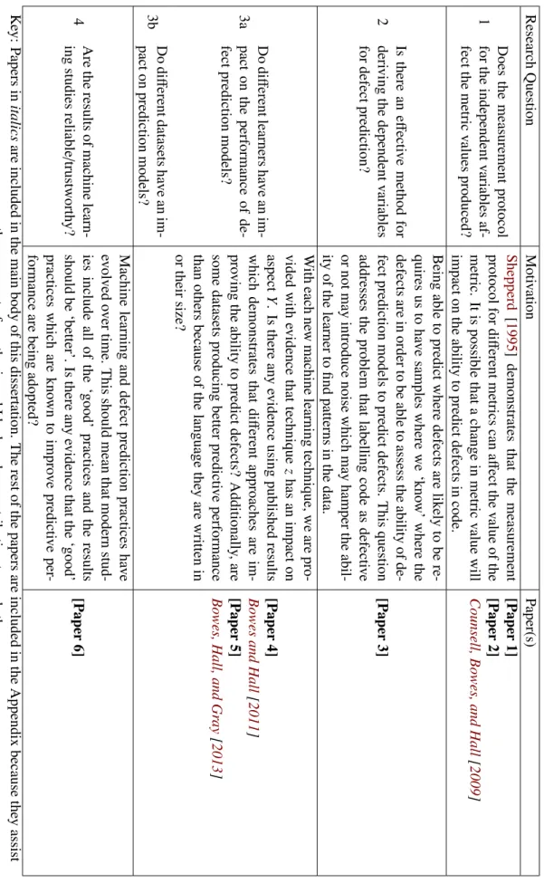
1.1 Research Questions . . . 4
2.1 Demonstration Data Where Each Line is for a Method Labelled as Defective or Not with Independent Variables: Method Return Type and Method Parameter Count. . . 12
2.2 Conditional Standard Deviation using Return Type . . . 14
2.3 Conditional Standard Deviation using Parameter Count . . . 14
2.4 Table of Methods Labeled as Defective or Not Based on the Return Type and Parameter Count. . . 16
2.5 Summary Table of Methods Labeled as Defective or Not Based on the Return Type and Parameter Count. . . 16
2.6 Hyper-Parameters for Some Learners. . . 23
2.7 Summary Statistics for NASA Datasets before Cleaning. . . 24
2.8 A Binary Confusion Matrix . . . 25
2.9 Compound Performance Measures from a Binary Confusion Matrix . . . 27
C
hapter
1
Introduction
1.1 Aim
Defects in code cost in excess of $50billion per year to put right in the US [Levinson 2001,Runeson and Andrews 2003]. Defect prediction is an important part of software engineering. It allows developers to prioritise the code that needs to be tested and inspected when trying to reduce the number of defects in code [Li et al. 2006]. Weyuker and Ostrand[2008] demonstrate that a small change in the number of defects found will have a significant impact on the cost of producing software.
Defect prediction techniques typically use training data to train a model which then predicts the defect proneness of a unit of code (module). Initially regression techniques were used to predict defects in code using static code metrics as the independent variables [Munson and Khoshgoftaar 1990]. More recently, Lessmann et al. [2008] demonstrate machine learning techniques being applied to predicting defects. With each new technique, the number of studies increases resulting in more than two hundred academic studies into defect prediction over the last ten years[Paper 4]1.
The aim of this dissertation is to demonstrate that the results of individual defect prediction studies risk not being comparable to other studies if not enough consideration has been given to how the dependent and independent variables have been computed. This dissertation will show that even when using the same source code to provide the independent variables and defect tracking data to produce the dependent variables, the way the defect data is extracted and processed may be different, which in some cases could be affecting the prediction results. Further, this dissertation aims to demonstrate that the performance measures used to justify the significance of the results can be confusing. Some reported performance values appear to be ‘good’, even though they could have been achieved by randomly predicting modules as defective [Shepperd 2013]. Finally, this dissertation will demonstrate that machine learning good practices are not always being applied which has a significant effect on the predictive performance of the models being built. The conclusion of this dissertation is that although the performance of defect prediction seems to have currently reached the limits of being able to predict defects [Menzies et al. 2008], many retrospective updates to previous experiments are needed in order to improve the reliability of the corpus of knowledge that already exists. In this dissertation I propose new techniques which allow researchers to analyse more easily the relative merit of the predictive performance of defect prediction studies.
1[Papern]refers to then’th paper which is part of the main argument of this thesis. A list of the 6 main papers can be
2 Chapter 1. Introduction
1.2 Introduction
Defects2in software are a side effect of creating a piece of code. Releasing code which contains defects can be costly and may threaten the confidence that users have in a system. This is exemplified by the recent problems which the Royal Bank of Scotland suffered with a system upgrade [Scott 2012]. The cost of fixing defects varies depending on the defect itself. It has been estimated that the cost of fixing defects in the US is between 50 and 78 billion dollars per year [Levinson 2001,Runeson and Andrews 2003]. Some defects are easier to fix than others, for example typos are relatively easy to find and easy to correct. Defects involving infrequently used pieces of code which require a high level of expertise to write may be more difficult to find than typos. The system domain also affects how easy defects are to fix. Defects in embedded systems tend to be more expensive to fix than defects in desktop applications [Turhan et al. 2009]. The size of the application is also likely to affect the ease with which defects can be found [Oram and Wilson 2010]. Part of the cost in fixing a defect is in the initial step of finding the defect. Historically, defects have been found during many stages of software development processes, including development and testing. Once a piece of software has been released, users may report defects. Locating where defects are will then involve many techniques, including automated methods and manual inspection which is costly. In summary, defects will occur, may need fixing and require varying amounts of time (and hence money) to fix.
Predicting where defects occur in software is an important area for research. Studies using automated techniques to determine where defects are have been published widely [Paper 4]. The aim of defect prediction is to reduce the amount of code that a software engineer needs to review in order to find a defect. Early techniques relied on simple regression techniques to associate code characteristics such as the number of Lines of Code (LOC) with the number of defects found. These studies have shown that relationships exist between code features and the presence of defects and have resulted in a continuous search for better ways to predict where defects are. Recently, machine learning has become a popular way of predicting which modules of code are defect prone. There have been more than 200 defect prediction studies carried out in the last decade[Paper 4]. These recent (2000 to 2010) studies are dominated by machine learning techniques3.
Menzies et al.[2008;2010] suggest that current defect prediction techniques have reached a limit to the percentage of defective code units that can be reliably predicted. This indicates that the field of defect prediction has matured and cannot be improved any further. This dissertation argues that although the results published by previous studies may have reached a ceiling, the results themselves may not be a true reflection of the ability of learners to identify where defects are with any degree of certainty. I will confirm the conjecture made byKitchenham et al. [1990] that there are many factors which can cause variation in the values of variables used in defect prediction studies. As a result of the variation, it may be necessary to re-work the published corpus of knowledge in defect prediction to gain a more precise understanding of the ability to reliably predict where defects are using different code characteristics. This dissertation will demonstrate that the measurement problems identified byFenton and Neil[1999], Kitchenham et al.[1990],Rosenberg[1997] are still current with regards to defect prediction studies:
“manual collection of data is itself error-prone...
2The term ’defect’ is used interchangeably in this dissertation with the terms ’fault’ or ’bug’ to mean a static fault in
software code. It does not denote a ’failure’ (i.e. the possible result of a defect occurrence while the system is executing).
1.3. Thesis and Research Questions 3
it is unreasonable to place much significance on relatively small effects, ... ” Kitchenham et al.[1990]
“Proper measurement based studies are the key to objective methods evaluation,” Fenton and Neil[1999]
1.3 Thesis and Research Questions
The thesis of this dissertation is that there are many factors which may affect the predictive performance of trainable models for software defect prediction. This thesis will be demonstrated by considering the following factors:
1. The independent variables. These are measures derived from the code and may include the number of lines of code (LOC) or the number of branch points in the module.
2. The dependent variables. These are usually either the number of defects in a module or a boolean value indicating if a module is defective or not defective.
3. The datasets and machine learners. The datasets are the combination of independent and depen-dent variables for a piece of software. The machine learner is the technique for building a model which can predict the dependent variables based on the independent variables.
4. The accepted machine learning approaches. These include the methods of calibrating the machine learners and measuring the performance of the model.
The main arguments of this thesis can be addressed by considering the research questions in Table1.1.
1.4 Contributions to Knowledge
This dissertation makes the following contributions to knowledge: Theoretical contributions
This dissertation makes two major theoretical contributions. The first contribution is the demonstration that the way that some independent variables (for example program slicing metrics) are computed affects the metric value (see[Paper 1],Bowes et al.[2011]4and[Paper 2]). This contribution means that it is necessary for studies to report how the metrics have been calculated if they are to be used in cross study comparisons. It also means that systematic literature reviews based on current work may need to exclude studies which have not reported the technique for gathering metric data. The second theoreti-cal contribution is imputing the observation that some machine learning practices (for example feature reduction techniques or data cleaning) do not appear to be being used systematically in recent defect prediction studies[Paper 6]. This may be due to poor reporting and means that it is important to report the detailed protocol used when performing defect prediction experiments using machine learning.
4 Chapter 1. Introduction Table 1.1: Research Questions Research Question Moti vation Paper(s) 1 Does the measurement protocol for the independent variables af-fect the metric values produced? Shepperd [ 1995 ] demonstrates that the measurement protocol for di ff erent metrics can a ff ect the value of the metric. It is possible that a change in metric value will impact on the ability to predict defects in code. [P aper 1] [P aper 2] Counsell, Bowes, and Hall [ 2009 ] 2 Is there an e ff ecti ve method for deri ving the dependent variables for defect prediction? Being able to predict where defects are lik ely to be re-quires us to ha ve samples where we ‘kno w’ where the defects are in order to be able to assess the ability of de-fect prediction models to predict defects. This question addresses the problem that labelling code as defecti ve or not may introduce noise which may hamper the abil-ity of the learner to find patterns in the data. [P aper 3] 3a Do di ff erent learners ha ve an im-pact on the performance of de-fect prediction models? W ith each ne w machine learning technique, we are pro-vided with evidence that technique z has an impact on aspect Y . Is there an y evidence using published results which demonstrates that di ff erent approaches are im-pro ving the ability to predict defects? Additionally ,are some datasets producing better predicti ve performance than others because of the language the y are written in or their size? [P aper 4] Bowes and Hall [ 2011 ] [P aper 5] Bowes, Hall, and Gr ay [ 2013 ] 3b Do di ff erent datasets ha ve an im-pact on prediction models? 4 Are the results of machine learn-ing studies reliable / trustw orth y? Machine learning and defect prediction practices ha ve ev olv ed ov er time. This should mean that modern stud-ies include all of the ‘good’ practices and the results should be ‘better’. Is there an y evidence that the ‘good’ practices which are kno wn to impro ve predicti ve per -formance are being adopted? [P aper 6] K ey: Papers in italics are included in the main body of this dissertation. The rest of the papers are included in the Appendix because the y assist the ar gument of my thesis and Ihad made a contrib ution to w ards them.
1.5. Structure of this Dissertation 5
Methodological contribution
This dissertation makes one major methodological contribution for generating a common set of pre-diction performance measures for binary classification prepre-dictions based on a wide range of measures reported in different studies (see[Paper 5]). This means that the performance results of current defect prediction studies can be compared even though they have not reported the same set of performance measures. It enables researchers to decide which performance measures to report in their studies if they want their results to be incorporated into a larger corpus of knowledge.
Practical contributions
This dissertation makes two minor practical contributions by providing two tools: (DConfusion see
[Bowes et al. 2013]in AppendixB) for recomputing the confusion matrix and (SLuRp seeBowes et al. [2012a] in Appendix B) for carrying out a systematic literature reviews. The first tool allows other researchers to check the consistency of their own results. The first tool also allows reviewers of defect prediction research papers to validate the reported results. The second tool is a web based tool which helps to manage the SLR process. SLuRp allows the reliable recording and moderation of researchers’ assessment of papers. SLuRp also integrates the tool for generating a common set of prediction perfor-mance measures extracted from the papers.
Data contribution
The secondary data collected from published defect prediction studies is reported in[Paper 4]. The dataset in[Paper 4]will allow researchers to study other factors such as the impact that research group has on the performance on defect prediction studies.
1.5 Structure of this Dissertation
The thesis of this dissertation is derived from a set of published papers which have been peer reviewed. Each paper makes a contribution to this dissertation by demonstrating either how different measure-ment protocols lead to variation in the metrics they produce or how variation in the machine learning approaches used impact on the predictive performance of defect prediction studies. The initial chapter gives a background to defect prediction. Later chapters describe the contributions of the published work to this dissertation.
The remaining part of this dissertation is organised as follows:
Chapter2gives an introduction to defect prediction and a brief summary of the current state of research in defect prediction.
Chapter3describes how the different published papers contribute to answering the research questions for this thesis. Chapter3ends with a description of my contribution to each paper. The contribution of the co-authors of each paper is also included.
Chapter4provides the peer reviewed published papers. Chapter4is composed of six sections, one for each of the main published papers.
C
hapter
2
A Summary of Defect Prediction
2.1 Introduction
This chapter is a review of defect prediction. It describes what a defect is, and why we should be interested in predicting where defects are. This chapter then details the data needed to build prediction models and the process of building models and measuring model performance.
2.2 What is a Defect?
The definition of a defect is best described by using the standard IEEE definitions oferror,de f ectand
f ailure [IEEE 1990]. Anerror1 is an action by a developer that results in ade f ect. A de f ect is the manifestation of anerrorin the code whereas a f ailureis the incorrect behaviour of the system during execution.
In summary:errordeveloper →defect→ f ailureruntime
2.2.1 What is the Purpose of Defect Prediction?
The practical purpose of defect prediction is to help identify modules of code which are defective by highlighting those modules which are defect prone in order to remove defects and hopefully reduce fail-ures2. When a failure is reported, programmers and/or testers may carry out manual inspection of the source code to find the defect(s). Code review is an expensive process on large systems. Weyuker and Ostrand estimate that on the large commercial systems they have studied, only 20% of a system can be effectively reviewed at a time [Oram and Wilson 2010]. The amount of code which has to be manually inspected can be reduced by using a variety of techniques. These techniques include program execution traces, source code visualisation (including program slicing) and defect prediction. Execution traces can help to identify the code running when the failure occurs and hence the code which is likely to be defec-tive. Program slicing can reduce the code comprehension problem further by allowing programmers to see the impact of code which leads up to a variable, and the impact a variable will have on future code execution [Weiser 1981;1979]. Defect prediction uses code features such as code complexity measures to predict areas of code which are more likely to be defect prone. The purpose of defect prediction is therefore to focus the programmer on potential hot spots in the code which are likely to contain defects.
1A developererrorcan also be defined as amistake[IEEE 1990].
2The removal of a defect may not remove any failure, because the end user may not use the functionality provided by the
8 Chapter 2. A Summary of Defect Prediction
Correctly identifying hotspots should improve the efficiency of programmers fixing defects and therefore improve the quality of the code.
2.2.2 What is Defect Prediction?
Defect prediction is the method of predicting where defects MAY be in a piece of code. When we talk about a defect predictor we are usually talking about a set of formulas or rules which allow us to assess how prone a unit of code is to having a defect in it.
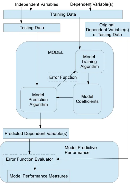
There are three main components of defect prediction: the independent variables which describe the code and what has happened to it (also known as the metrics), the dependent variable which describes the defectiveness of the code (sometimes called the label) and the model which is used to associate the independent variable to the dependent variable. The model is the part of the predictor which contains the equations and/or rules for predicting the dependent variable from the independent variables. The model is trained using historic data and an algorithm which derives the coefficients and decision rules. A function which determines how well the model fits the provided data is also required in order to be able to provide feedback to the trainer on how well the model fits the training data (see Fig2.1). A prediction function is used to predict dependent variables when presented with a set of independent variables from a test set with known labels for the defectiveness of each item. A second error function may be used to evaluate the performance of the model which can be used to compare one model against another. This second function does not have to be the same as the first error function used during training. In summary, the learner trains a model using training data, and the performance of the model is tested by predicting the defectiveness of test data which has not been used in the training set. Keeping the training and test data separate allows us to asses the ability of the model to predict future items with which the model has not previously been presented with.
2.2.3 Code Defects
Not all defects are the same. The set of defects which result from errors during coding are a subset of all possible defects which may cause a piece of software to fail. Defects can be characterised by where they come from, for example: code, configuration settings, hardware settings etc. Basili and Selby [1987] show that some defects are harder to find than others during testing. This suggests that some defects never leave the production line and are caught before the product is released. The post-release defects should have passed many of the tests created to trap defects before release and may therefore have different characteristics to pre-release defects [Radjenovi´c et al. 2013].
In this dissertation, I scope the definition of a defect to be: “in the source code”, because other defects are related to factors over which I had no control and were not discussed while carrying out the original studies reported in the main papers of this dissertation.
errorprogrammer →defect0code→ f ailureruntime
The scope of this dissertation is limited to defects in code which the developer can modify. I intend ignoring defects which are due to errors involving configuration files or any other settings for the soft-ware including the absence of: supporting libraries, an appropriate operating system or hardsoft-ware. It may not however be possible to limit the scope of this dissertation to defects in code because much research uses data derived from software systems which is not under the control of the researcher.Catal and Diri [2009] report that 60% of defect prediction datasets are based on commercial software. Companies are
2.2. What is a Defect? 9
Figure 2.1: A Diagram Showing How Dependent and Independent Variables are used to Build and Evaluate Models
reluctant to release source code for reasons of confidentiality and commercial advantage. Commercial companies are however occasionally happy to provide the software metrics which have been computed from the source code on the companies premises. For example, the NASA datasets3, currently located
10 Chapter 2. A Summary of Defect Prediction
in the PROMISE repository4, contain code metrics and the number of defects reported for closed source systems. Without the original source code or a detailed description of the measurement protocol of the closed source systems, it is not clear if the reported defects are code metrics or configuration defects. Hence it is not always possible to restrict the definition of defects todefect0
code5.
2.3 Variables Used in Defect Prediction Studies
The aim of defect prediction is to predict if a module of code is defect prone. As described earlier, the variables used to make the prediction (Lines of Code etc.) are called the independent variables and the predicted variable (defective or not, or the number of defects) is called the dependent variable. Both sets of variables need to be discussed further in order to be able to understand how they may impact on the models built and the performance of the models.
For the purpose of brevity, this dissertation will be limited to discussing variables as being either discrete or continuous. This is an oversimplification of variable types and the theory of scales of measurement which was first proposed byStevens [1946] and applied to software metrics by Fenton and Pfleeger [1997], Fenton [1991],Kitchenham et al. [1995], Morasca and Briand [1997], Shepperd [1988] and many others. Stevens [1946] proposed four types of measurement: nominal, ordinal, interval and ra-tio. Nominal measurement identifies items as belonging to a group or category. Ordinal measurement identifies items as belonging to a group, each of which can be placed in an order. Interval measurement identifies items as belonging to a group, each group can be ranked and the intervals between groups are the same. Ratio measurement is similar to nominal measurement with the added restriction that there is a zero value. Nominal, ordinal and interval measures together form the discrete measures and ratio measures form the continuous measures.
The measurement of software code was intensively studied during the 1970’s and the 1990’s byBaker et al. [1990],Fenton and Pfleeger[1997],Fenton [1991],Halstead [1977],Kitchenham et al.[1995], McCabe [1976], Morasca and Briand [1997],Shepperd [1988] and others. Baker et al. [1990] sum-marises the debate about software measurement and proposed a distinction between software measures and software metrics: metrics map the computed number to an ordering of the units, whereas measures result in values which are understandable and interpretable and consistent across different measurement protocols for the same measure.Baker et al.[1990] therefore allow length of a program to be considered as a measure because we have an intuitive understanding of what it means, and the length of different programs written in the same language can be compared and ordered. In this dissertation, I use the term metric rather than measure because the things being computed do not have a well defined common meaning. For example, in[Paper 2], we study how ‘code bad smells’ are identified and show that there is not a common understanding of what is meant by some of the common code bad smells.
4PROMISE is a well know repository of data used for defect prediction studies. The PROMISE repository [Menzies et al. 2012]http://code.google.com/p/promisedata/contains defect data for 40 projectsAs of 23/08/2012. Previous versions
of the repository can be found usingBoetticher et al.[2007],Shirabad and Menzies[2005].
5In this dissertation, I have been able to use the restricted definition (defect0
code) in[Paper 3]because the project being
2.4. Modelling Techniques 11
2.3.1 Independent Variables
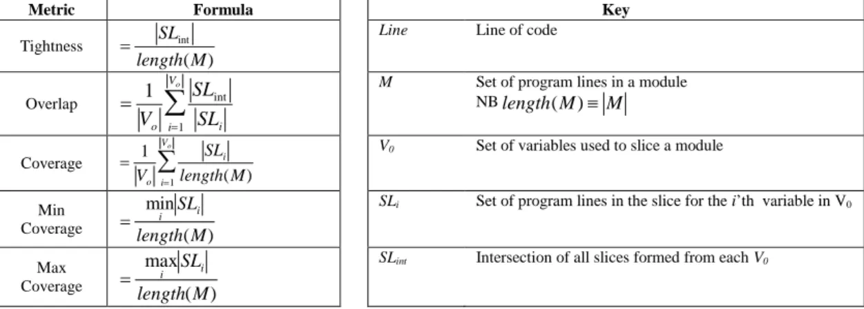
Independent variables are the set of variables used as the input for a model to make a prediction. They can be as simple as the number of Lines of Code, or as complicated as program slicing metrics such as tightness6 [Weiser 1979]. The independent variables are not confined to those which can be computed directly from the source code (sometimes referred to as static code metrics). Nagappan and Ball[2005] use a feature of software development called ‘churn’ which describes the amount of change in the code over time.Pinzger et al.[2008] describe how metrics based on the network of developers can be used to successfully predict defects. Many different independent variables have been used in defect prediction studies which are summarised in[Paper 4]and explained in detail in [Fenton and Pfleeger 1997].
2.3.2 Dependent Variables
The dependent variable, i.e. ‘defectiveness’ of the code being analysed, should be the output of defect prediction models. The variable can either be continuous (the ‘number of defects’ is frequently used by Weyuker et al. [2010]) or discrete (not defect prone or defect prone7). It is possible to convert a continuous variable into a discrete variable by splitting the data into ranges. For example,Menzies et al. [2007] binarises the NASA datasets into two ranges by labelling a module as not defect prone if the number of defects reported is zero otherwise the module is labelled as defect prone.
The initial labelling of the defectiveness of a module of code is perhaps the most difficult part of ac-quiring defect prediction data. There are many reasons which lead to defects being discovered in code including: manual inspection of code, failure of a test, failure report in a defect tracking system. Code inspection and test failure tend to happen pre-release and are dependent on developer effort. Identifica-tion of a defect due to a failure report happens post-release by users. The number of post-release defects will depend on how long the product has been released8and the number and diversity of users using the software. Latent defects will remain in the source code as long as either the failure is not reported or the code is not executed.
2.4 Modelling Techniques
The modelling technique is the method of building a model which associates the independent variable with the dependent variable. This allows a prediction of the unknown dependent variable of a new instance to be made. There are many different techniques available. Some techniques can deal with continuous data such as regression techniques and others can deal with categorical data such as Naïve Bayes . This next section describes a subset of techniques used in defect prediction studies. The subset of techniques presented here have been selected because they were used in the 36 studies identified in [Paper 4].
6Program Slicing metrics are defined later in[Paper 1].
7Other discretisation systems have been employed, for exampleKhoshgoftaar et al.[2005] uses a three way classification
of {not defect prone|low defect prone|high defect prone}
12 Chapter 2. A Summary of Defect Prediction
2.4.1 Continuous Techniques
There are a number of techniques which can predict the number of defects. Predicting the number of defects allows the developer to rank the modules by those which have the potential to have the most defects. Weyuker reports the Pareto effect [Newman 2005] is common with 20% of files containing 80% of defects [Oram and Wilson 2010, Chap. 9]. Weyuker also reports that inspecting 20% of the code is achievable in large systems. Therefore, as a software engineering exercise, ranking the modules by the number of defects and inspecting the top 20% is both practically achievable and likely to remove the greatest number of defects.
For the rest of the discussion on modelling techniques I will use a dummy data set to explain some of the techniques. The data is not real and has been constructed for demonstration purposes only. The data is based on a hypothetical analysis of some JAVA code where we are trying to predict the defect proneness of code by looking at the return type of a method and the number of parameters in the method signature. The data is presented in Table2.1.
Table 2.1: Demonstration Data Where Each Line is for a Method Labelled as Defective or Not with Independent Variables: Method Return Type and Method Parameter Count.
RowId Return Type Parameter Count Defect Count
1 void 1 0 2 void 2 0 3 void 1 0 4 void 2 0 5 void 2 0 6 void 2 0 7 void 4 0 8 void 2 0 9 int 0 0 10 boolean 1 0 11 void 1 2 12 int 4 4 13 ArrayList 8 8 14 JFrame 0 100 2.4.1.1 Regression
Regression techniques are based on a single mathematical equation. The equation has the dependent variable on one side and the independent variables on the other. A simple example of a regression model would be:
D=c0+c1×PC (2.1)
WhereDis the predicted number of defects,PCis the number of parameters passed to the method. c0 andc1are constants and can be estimated using:
2.4. Modelling Techniques 13 c0= ( PD)(PPC2) −(PPC)(PD ×PC) n(PPC2) −(PPC)2 (2.2) c1 = n( PD ×PC)−(PPC)(PD) n(PPC2) −(PPC)2 (2.3)
Equations2.2and2.3produce values ofc0andc1which minimise the following error function
S umsO f S quares=X
(PC−D)2 (2.4)
Multiple regression involves variables being added to the right of Equation2.5e.g.:
D=c0+c1×PC+c2×r (2.5)
Whereris 1 if the return type is void and 0 if the return type is not void. The constants can be calibrated to reduce the error by reformulating the above equation for each instanceiof the training data:
Di=c0+c1×PCi+c2×ri+εi (2.6)
Whereεis an error term for the particular instance. Wheni>v(v=the number of variables), it becomes possible to determine the coefficientsr0...rv by solving the set of simultaneous equations.
Negative Binomial Regression (NBR) is an especially useful regression technique for studies which use the number of defects per module as the dependent variable [Oram and Wilson 2010, Weyuker et al. 2010]. NBR is based on linear regression but uses a log transformation of the dependent variable, i.e. the log of the number of defects against the linear form from above, for example Equation2.7.
loge(D)=c0+c1×PC+c2×r (2.7)
2.4.1.2 Regression Decision Trees
Regression decision tree techniques are based on a simple tree model. A decision tree is composed of nodes which contain decision logic. The decision may be made on a single attribute of the independent data for example LOC > 4 which splits the data into different ranges. For each range the node will either lead to another node or to a final decision for example 5 defects. A tree is used by presenting the independent variables to the starting root node which then makes a decision. The attributes are passed down to other nodes until a final decision is made.
Choosing the variable to split the data on is done by observing the standard deviation of the dependent variable before the split and comparing it to the combined standard deviations of the data after the split using one of the independent variables.
Equation2.8is the usual equation for calculating the standard deviation of the original population:
S(x)= v u t 1 N N X i=1 (xi−µ)2 (2.8)
14 Chapter 2. A Summary of Defect Prediction Where µ= 1 N N X i=1 xi (2.9)
The combined standard deviation of the data after a potential split is calculated as follows:
S(T,X)=X
c∈X
P(c)S(c) (2.10)
Using the data from Table2.1.S =25.5730
If we split on the return type we get a standard deviation of 0.6898 (Table2.2). Table 2.2: Conditional Standard Deviation using Return Type
Return Type Probability Std.Dev. Combined
void 9/14 0.6285 0.4041 int 2/14 2.0000 0.2857 boolean 1/14 0.0000 0.0000 ArrayList 1/14 0.0000 0.0000 JFrame 1/14 0.0000 0.0000 Total 0.6898
Splitting the data on the number of Parameters>0, we get a standard deviation of 9.1783 (Table2.3). Table 2.3: Conditional Standard Deviation using Parameter Count
Parameter Count Probability Std.Dev. Combined
0 2/14 50.0000 7.1429
>0 12/14 2.3746 2.0354
Total 9.1783
This shows that the standard deviation after splitting onReturntypeis less than the standard deviation after splitting onParametercount. The lower standard deviation forReturntypeindicates that it would be better to split onReturntypethanParametercountbecause the items in the groups formed by splitting onReturntypeare more alike than items found in groups by splitting onParametercount. When the data can no longer be split, the average value of the dependent variable is reported.
2.4.2 Categorical Techniques
Sometimes we do not know the number of defects, we only know if the module is defective or not defective. Fortunately categorical techniques can predict variables with values on the nominal scale. In the case of defect prediction, this would be either not defect prone or defect prone. Many techniques exist for solving this problem which are detailed below.
2.4. Modelling Techniques 15
2.4.2.1 Statistical Methods
Logistic regression is a technique which produces a probability that the output is either 0 or 1. It uses a non linear equation based on the sigmoid function (see Equation2.11).
g(z)= 1
1+e−z (2.11)
The probability that the output is 1 is given by:
Pr[y=1|x;θT]= 1
1+e−f(x,θT) (2.12)
Where f(x, θT) is an expression such asθ
0+θ1x1+θ2x2+θ3x3andθT is a vector of constants andxis a vector of variables withx0=1 (i.e. the intercept).
θT is found by repeatedly updating the coefficients using Equation2.13until the change in error after updating the coefficients is less than a pre-determined threshold value.
θ0 j:=θj+α m X i=1 (f(X(i), θT)−Y(i))X(ji) (2.13) For clarity:
Xis a vector of vectors of independent variables.
θjis the j’th value ofθ.
αis a constant which defines the learning rate.
mis the number ofXvectors.
iis a variable to indicate which of themvectors ofXis being used.
Yis the label for thei’th vector.
Naïve Bayes is a statistical technique based in the probability theories of Thomas Bayes. It uses the following probability equation:
Pr[H|E]= Pr[E|H]Pr[H]
Pr[E] (2.14)
WherePr[H|E] means the probability of classHbased on the probability of classesE.
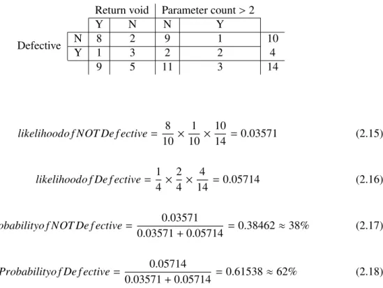
Naïve Bayes assumes that the independent variables are independent of each other (which is rarely the case) and that the presence of each independent variable has a different contribution to the probability of each dependent category (from now on called the class9). A simple example will help at this point. Consider the problem of predicting if a module is defective. We will use the data in Table2.1 which is further summarised Table2.4 and Table2.5. Note that Naïve Bayes can only deal with categorical variables, therefore the count of the number of parameters has been binarised with a threshold of 3 or more, and defectiveness has been binarised with a threshold of 1 or more indicating defectiveness. If we have a new method with a return type ofvoidand 5 parameters in the method call we do not know Pr[E]. We can however compute the probability of the method being defective using Equations2.15 and2.16resulting in Equations2.17and 2.18:
16 Chapter 2. A Summary of Defect Prediction
Table 2.4: Table of Methods Labeled as Defective or Not Based on the Return Type and Parameter Count.
RowId Defective Return void Parameter count>2
1 N Y N 2 N Y N 3 N Y N 4 N Y N 5 N Y N 6 N Y N 7 N Y Y 8 N Y N 9 N N N 10 N N N 11 Y Y N 12 Y N Y 13 Y N Y 14 Y N N
Table 2.5: Summary Table of Methods Labeled as Defective or Not Based on the Return Type and Parameter Count.
Return void Parameter count>2
Y N N Y
Defective NY 81 23 92 12 104
9 5 11 3 14
likelihoodo f NOT De f ective= 8
10 × 1 10 × 10 14 =0.03571 (2.15) likelihoodo f De f ective= 1 4× 2 4 × 4 14 =0.05714 (2.16)
Probabilityo f NOT De f ective= 0.035710.03571+0.05714 =0.38462≈38% (2.17)
Probabilityo f De f ective= 0.035710.05714+0.05714 =0.61538≈62% (2.18) Showing that the probability of a method with a void return and more than two parameters being de-fective is 62%. On the balance of probability, we will predict this method as being dede-fective. Naïve Bayes does give us some idea of the certainty that the method will be defective which is lost in the final
2.4. Modelling Techniques 17
classification based on the balance of probability. Naïve Bayes uses categorical data for all variables which is incompatible with LOC for example. This incompatibility is overcome by discretising none categorical data.
2.4.2.2 Classification Decision Trees
Classification decision tree techniques are another example of a tree model. Classification decision trees use InfoGain [Quinlan 1993] or Gini [Breiman et al. 1984] as the measure of how much a split is better when using a particular variable to split the data on. There are many implementations of decision classification decision tree techniques such as c4.5, J48, and rpart [Breiman et al. 1984,Quinlan 1993, Witten and Frank 2002].
For the rest of this section we will consider c4.5 as our example. c4.5 is a tree technique developed by Quinlan[1993]. c4.5 uses the measure called information entropy to decide which variable should be used at a node to divide up the data. The variable which results in the highest InfoGain is used at a node to split the data. InfoGain is the difference between the entropy of the original data and the conditional entropy of the data using a particular variable. Information entropy is a measure of how uniformly distributed different classes are in a population and was first proposed byShannon and Weaver[1948]. For example, if we have a dataset with 10 instances and 5 are defective and 5 are not defective, the entropy is 1. If all of the values are the same, entropy is 0. The formula for entropy is:
H(X)=− n
X
j=1
pjlog2(pj) (2.19)
Consider the example data in Table2.4, there are 10 none defective items and 4 defective items. The entropy of this data is:
H(De f ective)=−10 14log2 10 14 ! − 4 14log2 4 14 ! =0.3467+0.5164=0.8631 (2.20)
If we decide to split the data into two groups using the Return is void variable, we get:
H(De f ective|ReturnIsVoid)=−8 9log2 8 9 ! − 1 9log2 1 9 ! =0.1510+0.3522=0.5033 (2.21) H(De f ective|ReturnIsNotVoid)=−2 5log2 2 5 ! − 3 5log2 3 5 ! =0.5288+0.4422=0.9710 (2.22) The conditional entropy is the combined entropy of the two groups formed by splitting the data using the Return type variable. A low conditional entropy indicates that the groups are uniform, i.e. the items in the group are similar to each other. For the Return type, the conditional entropy is given by:
H(De f ective|ReturnType)=0.5033 9 9+5 ! +0.9710 5 9+5 ! =0.6703 (2.23)
If we consider splitting the data using the Parameter count variable we get:
H(De f ective|ParameterCount ≤2)=− 9 11log2 9 11 ! − 2 11log2 2 11 ! =0.2369+0.4472=0.6840 (2.24)
18 Chapter 2. A Summary of Defect Prediction H(De f ective|ParameterCount>2)=−1 3log2 1 3 ! − 2 3log2 2 3 ! =0.5283+0.3900=0.9183 (2.25) The conditional entropy using Parameter count variable is given by:
H(De f ective|ParameterCount)=0.6840 11 14 ! +0.9183 3 14 ! =0.7342 (2.26)
InfoGain is a measure of how much information has been gained by splitting the data using a variable. InfoGain is the difference between the original entropy (Equation2.20) and the conditional entropy for the variable (for example Equation2.26).
In f oGain(ReturnType)=0.8631−0.6703=0.1928 (2.27)
The InfoGain using Parameter count variable is given by:
In f oGain(ParameterCount)=0.8631−0.7342=0.1289 (2.28) This suggests that the best variable to split the data on is the Return type=voiddecision. Having split the data, the above technique is applied to both sub groups until the entropy of the group is 0 or some other stopping condition is met. This repetitive splitting is called recursive partitioning.
A c4.5 learner can also try to simplify the tree produced using a technique called pruning, so that there are fewer branches or nodes with single items. c4.5 can use continuous independent variables by deter-mining a threshold value of the variable to split on. J48 is a JAVA implementation of c4.5. J48 produces the tree seen in Fig.2.2for the data found in Table2.4.
Random ForestTMis an ensemble technique which uses a collection of decision trees [Breiman 2001]. The dataset for each tree is created using a technique called bagging. Bagging involves randomly select-ing a subset of independent variables from the original data set and then randomly selectselect-ing instances from the dataset with replacement. This creates a variety of models which perform differently for an item of data drawn from the original dataset. When a new item of data is presented to the Random For-est model, the predictions for each tree are aggregated together to form a collective decision. Random Forest techniques have been shown to work well for defect prediction studies [Lessmann et al. 2008].
2.4.2.3 Other Techniques
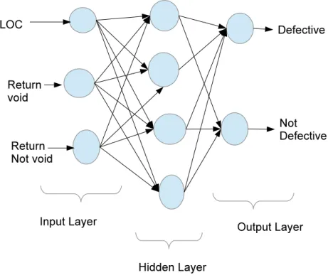
Artificial Neural Networks (ANN) are a technique which use parallel decision units which take input data and produce an output which may form the input of other decision units. A typical ANN uses a unit called a perceptron as the decision unit. The input to a perceptron is multiplied by a coefficient called a weight. The output of a perceptron is a function of the sum of the weighted inputs. An ANN is trained by repeatedly presenting input data to the ANN and then adjusting the weights using a method called back propagation. This is similar to the updating of coefficients described for logistic regression. Different arrangements of networks exist, the most common is a feed forward network with three layers: the input layer, the hidden layer and the output layer (see Fig. 2.3). It should be noted that the number of perceptrons in the hidden layer can be altered. Altering the size of the hidden layer has been observed to alter the ability of the network to predict the required outputs [Hertz et al. 1991]. The learning rate, the momentum of learning and the number of times the data is presented to the network for learning (epochs) are also known to have an impact on the ability to predict new items [Salehi et al. 1998].
2.4. Modelling Techniques 19
Figure 2.2: J48 Tree for the Simple Defect Data Found in Table2.4.
The values in brackets e.g. (9.0/1.0) shows the number of items in the group and the number which are incorrectly classified.
20 Chapter 2. A Summary of Defect Prediction
Support Vector Machines (SVM) were developed byVapnik[1963]. SVMs identify a separating plane which maximises the ‘distance’ between the plane and the vectors which are closest to it for linear separation problems. Boser et al. [1992] introduced the kernel trick which extended the capability of SVMs to allow solutions for non-linear problems. The kernel trick uses different functions to map the original data to a higher number of dimensions which when projected onto the original space form non linear surfaces. Such tricks usually require hype-parameters, for example the radial base function has a
γ coefficient. Cortes and Vapnik[1995] extended the technique to allow the misclassification of some items by adding a cost coefficientC. High values ofCresult in fewer training items being misclassified by building a more complex model. SVMs work best when the coefficients for exampleC andγ(for radial base kernel function) are optimised. Optimisation may involve a grid search which builds models using a grid ofC andγvalues. Tabu searches [Glover 1989;1990,Glover and McMillan 1986] have been used with success recently to find the optimal coefficients for SVM coefficients [Corazza et al. 2010].
K-Nearest Neighbour (kNN) is a simple technique which takes the average label for theknearest neigh-bours. For continuous independent data the Euclidian distance is used to measure the distance from the test item to the possible nearest neighbours. For categorical independent variables, the Hamming distance can be used as a measure of distance. Producing a good kNN model requires finding the best value ofkwhich can be achieved by increasing the value ofkfrom 1 to some maximum value.
2.5 Data Quality and Data Cleaning
Witten and Frank [2005] states that machine learning should be tolerant of noise in the data. Some learners such as Naïve Bayes can make predictions in the presence of noise. It is possible to use this argument that learners can cope with noise to justify ignoring the need for data cleaning. Recently, Gray et al.[2012] identified noise in the NASA datasets which could not have been computed from the raw data (for example 1.1 LOC) and should have been removed before being used in defect prediction studies. NASA data has been used by over 30 different studies, with only one other study [Boetticher 2006] making any comment about the incorrect data items. Data cleaning and simply eye-balling the data appears to have become a forgotten part of the researchers’ protocol.Gray et al.[2012] describes a sensible approach to cleaning the static code metrics of datasets used for defect prediction.
2.6 Model Building Approaches
This section describes the approaches used to build models which will work on data which has not been used to build the model. Model building approaches involve creating training and test data, as well as dealing with issues such as data quality.
2.6.1 Building Generalisable Models
Building a model which can correctly label the training set is important, however good models should have additional characteristics. Fenton and Neil[1999] describes the two aims of building prediction models as 1) building models which will correctly predict ‘new’ data (generalisability) and 2) building models which are understandable (comprehensibility). Some models are able to generalise the predic-tion problem to correctly predicting modules they have never seen before. Building models which can generalise well will depend on what data is used to train the model and what error function is used to
2.7. Issues of Model Building Specific to Machine Learning 21
determine how well the model performs and how the model is built [Gray 2013,Witten and Frank 2005]. Different leaners produce models of different comprehensibility. Decision trees are simple to interpret and SVMs are difficult10.
Feature reduction is sometimes applied to the independent variables to simplify the learning process, to remove highly correlated data and to build more generalisable models. Menzies et al.[2007] demon-strated that it is possible to achieve relatively good performance on a highly reduced set of independent variables. Feature reduction can be achieved by removing attributes which have a low entropy (see Equation2.19) and/or a high correlation with other independent variables.
2.6.2 Testing the Generalisability of Models
Testing the generalisability and hence the validity of a model involves testing it on some ‘new’ data. If the model can continue to perform well on ‘new’ data it can be considered to have been able to generalise the problem.
In software engineering, the new data could come from the next release of a software product [Weyuker et al. 2010]. Using the next release to check the model is called cross-release validation.
Some researchers also assess the performance of their models on data from different system because they want to know if a model is transferable to a wider range of environments. Testing models on different systems is called cross project validation and in defect prediction rarely works well [Turhan et al. 2009, Zimmermann et al. 2009].
The availability of data for performing cross project validation is has increased with the availability of online repositories. The PROMISE repository has made available defect data from many different systems which should allow cross project validation. Some datasets, for example, those for the Eclipse JAVA IDE development tool are available for different releases allowing cross-release validation to take place.
In the absence of data for different systems and different releases, it is possible to perform model val-idation by splitting the entire dataset into folds (sets of instances) and keeping one fold as the test set and the rest as the training set. This splitting of the data into folds in order to produce training and testing sets is called n-fold cross validation (wherenis the number of folds). Problems can occur when forming the folds with highly imbalanced data. It is possible that some folds may not have any instances of the minority class. Having no instances of a particular class causes problems when measuring the performance of a model because the divisor of some measures is the total number of that class, hence the performance measure has a divide by zero problem (see Table2.9for the formula for different per-formance measures). To overcome this, the folds should have roughly the same distribution of each class as the original population, i.e the folds are stratified.
2.7 Issues of Model Building Specific to Machine Learning
Machine learning techniques are affected by both internal settings and the charactersistic of the data they are being trained on. The major issues are discussed below.
10The use of Support Vector Inductive Logic Programming combines SVMs with a technique called inductive logic
22 Chapter 2. A Summary of Defect Prediction
2.7.1 Dealing with Datasets which are Unbalanced
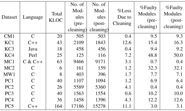
Most datasets used by defect prediction studies have few instances of the defective class in them (i.e. they are unbalanced). We would hope that this would be the case since defects are normally a bad thing. If we look at the NASA datasets in Table 2.7 we can see that the percentage of defective instances ranges from 0.4% in PC2, to 48.8% for KC4. The imbalance of most datasets changes after cleaning (see Table2.7). Unfortunately the lack of instances which are labelled as defective does not help the learner. The learner c4.5 is thought to struggle with imbalanced data ([Japkowicz and Stephen 2002] and [Liu et al. 2010]) and this may explain the poor performance of models found inArisholm et al. [2007;2010]. For techniques which are sensitive to imbalanced datasets, there are two ways of making the training set11more balanced. These include under-sampling the majority class or oversampling the minority class. Under-sampling involves selecting all items from the minority class and then randomly picking the same number of items from the majority class. Over-sampling involves synthetically creating extra examples from the minority class. SMOTE is an over-sampling technique which creates new items from the minority class by taking two ‘close’ items a third synthetic item with independent variable values which lie between the independent variables of the two items [Chawla et al. 2002].
2.7.2 Machine Learning Model Optimisation
Model optimisation is the process of finding the set of parameters for a learner which achieves a good predictive performance on the training set (for example the cost coefficient of SVMs needs to be opti-mised for different datasetsGray et al.[2010]) . During model optimisation, the algorithm which trains the model has to ‘know’ what is good performance and what is bad performance. Model optimisation algorithms search for models which minimise an error function such as Mean Magnitude of Relative Error (Equation2.30) for continuous dependent variables or Accuracy (Equation2.31) for categorical dependent variables. Different error functions can be used depending on the purpose of the model. Some error functions are not always appropriate.Miyazaki et al.[1994] show that MMRE is lower for models which underestimate, andFoss et al. [2003] show that MMRE can lead to counterintuitive examples. Lokan[2005] studied different error functions and concluded that functions which minimise actual error perform better than functions which minimise relative error. Port and Korte[2008] show that MMRE (see Equation 2.30) is more sensitive to outliers than PRED (see Equation2.32) as a measure of er-ror. Accuracy (see Equation2.31) should not be used as an optimisation function with imbalanced data because good values of accuracy can be achieved by simply predicting the majority class. A model opti-mised for Recall can be produced by making every prediction the preferred class (e.g. defective). Recent work byShepperd[2013]12would recommend using Mathews Correlation Coefficient (MCC see Table
2.9) as a measure of model accuracy because it is less biased to measuring the predictive capability on a particular class. Rezwan et al.[2013] also show that a binary classifier achieves better results when optimised on the same performance measure that will be used for the final performance measure.
MRE= |yi− prediction(xi)|
yi (2.29)
11Only the training set needs to be adjusted, because the performance of the final model should be representative of the
original data.
12The recent work byShepperd[2013] is based on the data we have extracted from[Paper 4]. Both Myself and Tracy Hall
2.7. Issues of Model Building Specific to Machine Learning 23
Technique Coefficients to Tune
Naïve Bayes Can be used without setting any initial coefficients. Random Forest Depth of Tree and min nodes per leaf
SVM Candγ
kNN kthe number of nearest neighbours
Neural Networks The number of nodes in each hidden layer, the number of hidden layers,the level of connectivity between layers.
Table 2.6: Hyper-Parameters for Some Learners.
MMRE= N1 N X i=1 |yi−prediction(xi)| yi ! (2.30) Accuracy= itemscorrect N (2.31) 2.7.3 Model Tuning
In order to produce good performance, some learners need tuning. Some learners (SVMs, RandomFor-est) have hyper-parameters which can be altered and will affect the ability to effectively learn a particular data set. Tuning involves searching for the best hyper-parameters either in a systematic manner for ex-ample a grid search or some other way such as a Tabu search [Corazza et al. 2010]. During the search, the training data is split into folds. Each fold is then used in turn as a validation fold, with the other folds being used to train a learner with a set of hyper-parameters. The performance on each validation set is then measured and averaged for all validation folds. The hyper-parameters which produce the highest average performance (or least error) are then chosen to build a model on the entire training set. Algorithm 1is taken from Rezwan et al. [2013] and succinctly describes a typical tuning setup for a SVM. Note that in the algorithm, data items which have the same values for the independent variables but different labels for the dependent variable13 are removed because they hinder SVMs in their ability to produce a suitable separating hyperplane. Table2.6describes some of the meta-parameters which can be altered for different learners.
2.7.4 Reordering the Training Data
Some learners will produce different results with the same dataset because the order in which the items are presented to the learner will affect the model. Witten and Frank [2005] report that the clusters produced for the famous Iris (plants) dataset are highly dependent on the ordering of the items presented to the learner. It is therefore common for the training set to be reordered after creating the training and testing sets from the different folds (as seen in Algorithm1).
24 Chapter 2. A Summary of Defect Prediction
Algorithm
Remove all inconsistent and repeated data points;
Split the data into two-third training from the new data set, one-third test from the original data set. Split the training data into 5 partitions;
This gives 5 different training (four-fifth) and validation (one-fifth) sets. The validation set is drawn from the original data set;
Use sampling to produce more training sets with equal numbers of each class; foreach pair of C/γSVM hyper-parametersdo
foreach of the 5 training setsdo Train an SVM;
Measure performance on the corresponding validation set, exactly as the final test will be measured. So use the Performance Measure, after the predictions on the validation set have been filtered;
end
Average the Performance Measure over the 5 trials; end
Choose the hyper-parameter C/γpair with the best average Performance Measure;
Pre-process the complete training set and train an SVM with the best C/γcombination Test the trained model on the unseen test set;
Post-processing the final prediction ;
Algorithm 1: Finding the best hyper-parameters with modified cross-validation method taken from [Rezwan et al. 2013].
Table 2.7: Summary Statistics for NASA Datasets before Cleaning
Dataset Language KLOCTotal
No. of Mod-ules (pre-cleaning) No. of Mod-ules (post-cleaning) %Loss Due to Cleaning %Faulty Modules (pre-cleaning) %Faulty Modules (post-cleaning) CM1 C 20 505 503 0.4 9.5 9.3 KC1 C++ 43 2109 1843 12.6 15.4 16.3 KC3 Java 18 458 456 0.4 9.4 9.2 KC4 Perl 25 125 116 7.2 48.8 50.0 MC1 C & C++ 63 9466 9171 3.1 0.7 0.4 MC2 C 6 161 159 1.2 32.3 32.1 MW1 C 8 403 396 1.7 7.7 7.1 PC1 C 40 1107 1094 1.2 6.9 6.4 PC2 C 26 5589 5360 4.1 0.4 0.4 PC3 C 40 1563 1554 0.6 10.2 10.0 PC4 C 36 1458 1396 4.3 12.2 12.6 PC5 C++ 164 17186 15278 11.1 3.0 3.1
2.8. Measuring the Performance of a Model 25
2.8 Measuring the Performance of a Model
Having produced a model on a dataset, we would like to know how it performs on ‘new’ data. Cross-validation described earlier provides a mechanism for providing the ‘new’ test sample, but does not give us an indication of the performance. Measuring the performance of a learner on the test set is an important aspect of defect prediction because it gives us some idea of how good a model/technique is on a particular dataset. The performance measures which have commonly been used in the past to measure model performance can be categorised into two groups based on whether the de