Face Detection and Verification using Local Binary Patterns

(1)

Face Detection and Verification

using Local Binary Patterns

THÈSE No_{3681 (2006)}

PRESENTÉE LE 26 OCTOBRE 2006

Á LA FACULTÉ DES SCIENCES ET TECHNIQUES DE L’INGÉNIEUR Laboratoire de l’IDIAP

SECTION DE GÉNIE ÉLECTRIQUE ET ÉLECTRONIQUE

ÉCOLE POLYTECHNIQUE FÉDÉRALE DE LAUSANNE

POUR L’OBTENTION DU GRADE DE DOCTEUR ÈS SCIENCES

PAR

Yann RODRIGUEZ

ingénieur en microtechnique EPF

de nationalité suisse et originaire de Bagnes (VS)

acceptée sur proposition du jury: Prof. J.R. Mosig, président du jury

Prof. H. Bourlard, Dr. S. Marcel, directeurs de thèse Prof. T. Cootes, rapporteur

Prof. M. Pietikäinen, rapporteur Prof. J.-Ph. Thiran, rapporteur

Lausanne, EPFL 2006

(2)

(3)

Abstract

This thesis proposes a robust Automatic Face Verification (AFV) system using Local Binary Pat-terns (LBP). AFV is mainly composed of two modules: Face Detection (FD) and Face Verification (FV). The purpose of FD is to determine whether there are any face in an image, while FV involves confirming or denying the identity claimed by a person. The contributions of this thesis are the following: 1) a real-time multiview FD system which is robust to illumination and partial occlusion, 2) a FV system based on the adaptation of LBP features, 3) an extensive study of the performance evaluation of FD algorithms and in particular the effect of FD errors on FV performance.

The first part of the thesis addresses the problem of frontal FD. We introduce the system of Viola and Jones which is the first real-time frontal face detector. One of its limitations is the sensitivity to local lighting variations and partial occlusion of the face. In order to cope with these limitations, we propose to use LBP features. Special emphasis is given to the scanning process and to the merging of overlapped detections, because both have a significant impact on the performance. We then extend our frontal FD module to multiview FD.

In the second part, we present a novel generative approach for FV, based on an LBP description of the face. The main advantages compared to previous approaches are a very fast and simple training procedure and robustness to bad lighting conditions.

In the third part, we address the problem of estimating the quality of FD. We first show the influence of FD errors on the FV task and then empirically demonstrate the limitations of current detection measures when applied to this task. In order to properly evaluate the performance of a face detection module, we propose to embed the FV into the performance measuring process. We show empirically that the proposed methodology better matches the final FV performance.

Keywords:Face Detection and Verification, Boosting, Local Binary Patterns.

(4)

(5)

Résumé

Cette thèse présente un système d’authentification biométrique basé sur la reconnaisance de visage. Le système est composé de deux modules: détection et authentification. Le but du premier module consiste à détecter si un visage est contenu dans l’image. Le second module détermine si ce visage appartient ou non à la personne qui tente de s’authentifier. Les contributions de cette thèse sont les suivantes: 1) un module de détection temps-réel robuste à lumière et capable de localiser des visages non frontaux, 2) un module d’authentification basé sur l’adaptation de filtres locaux appelés LBP (Local Binary Pattern), 3) une étude sur l’évaluation de la qualité des modules de détection.

La première partie de ce travail discute le problème de la détection de visages. Les principales limites des systèmes existants résident dans le manque de robustesse à la lumière et aux occulta-tions partielles du visage. Pour y remédier, nous proposons une représentation du visage basée sur les LBP. Une attention particulière est apportée aux processus de recherche dans l’image et de la fusion des multiples détections, qui peuvent avoir un impact significatif sur les performances du système.

Dans la deuxième partie, nous présentons une nouvelle méthode d’authentification, basée sur une représentation LBP de l’image. Elle offre une meilleure robustesse aux conditions de lumière et une procédure d’entrainement plus simple et rapide.

La troisième partie adresse le problème de l’évaluation de la qualité de la détection de visages. En premier lieu, nous analysons l’influence des erreurs de détection sur l’authentification. Ensuite, nous démontrons empiriquement les limites des mesures de détection existantes, puis nous pro-posons d’encapsuler le module d’authentification dans le processus d’évaluation. La méthodologie proposée améliore l’évaluation de la performance finale du module d’authentification.

Mots-clés:Détection et authentification de visages, Boosting, Local Binary Patterns.

(6)

(7)

Acknowledgement

The research presented in this thesis has been carried out at the IDIAP Research Institute in Martigny, between the years 2002 and 2006, under the supervision of Dr. Sébastien Marcel and Dr. Samy Bengio. I would like to thank them for their guidance, availability and enthusiasm dur-ing this thesis. It was great to work with them. Many thanks to Sébastien who always support me along these four years. Beside the hot discussions about C++ code cleaning and Torchvision data management, I will keep very nice memories of the CeBIT (darts, box of cookies, Japanese restau-rant..) and also of the wonderful "Médaillon de cerf" we had after the private defense! I would also like to thank IDIAP for funding my research and Prof. Hervé Bourlard for his encouragement and valuable advice.

Thanks to my officemates and colleagues at IDIAP over the years, and especially to Agnes for the interesting discussions, for sometimes being my secretary, for helping me when I was desperate with latex and generally for the nice working atmosphere. Special thanks to Ronan and Johnny for their C++ support and teaching in machine learning. I do not want to forget Frank, Norbert and Tristan of the system group, always available, efficient and very nice guys.

I would like to thank the jury members of my thesis committee for the many interesting com-ments and criticism that helped improve this manuscript.

Lastly and most importantly, I am deeply grateful to my lovely parents and my brother for their unconditional support, and to Sandra for her encouragement, her smile, her delicious food and her constant love.

(8)

(9)

List of Figures

1.1 Structure of an automatic face verification system . . . 4

2.1 Five types of Haar-like features . . . 12

2.2 Haar-like feature computation with the integral image . . . 13

2.3 Overview of the cascade architecture . . . 14

2.4 Extended Haar-like feature set (1) . . . 16

2.5 Extended Haar-like feature set (2) . . . 16

2.6 The basic Local Binary Pattern operator . . . 19

2.7 Robustness of the LBP features . . . 19

2.8 The extended LBP operator with (8,2) neighborhood . . . 20

2.9 Pixel classifier and its associated look-up table . . . 21

2.10 Face criterion . . . 23

2.11 Face anthropometric measures . . . 25

2.12 Virtual face training examples . . . 26

2.13 Nonface training examples . . . 26

2.14 Image examples of the XM2VTS database (standard set) . . . 27

2.15 Image examples of the XM2VTS database (darkened set) . . . 27

2.16 Image examples of the BioID database . . . 28

2.17 Image examples of the Purdue database . . . 29

2.18 Overlapped detections merging . . . 30

2.19 Performance evaluation on the XM2VTS database . . . 33

2.20 Performance evaluation on BioID and BANCA databases . . . 34 xi

(14)

2.21 Performance evaluation on the Purdue database . . . 36

2.22 Influence of the merging parameters . . . 37

2.23 Influence of the training set size . . . 38

3.1 Different architectures of multiview face detection systems . . . 43

3.2 Overview of the architecture of the multiview face detector . . . 45

3.3 In-plane and out-of-plane view partitions . . . 46

3.4 Overview of the architecture of the out-of-plane detector . . . 46

3.5 Overview of the architecture of the in-plane detector . . . 47

3.6 Merging overlapped multiview face detections . . . 50

3.7 Output of the multiview face detector illustrating the merging process . . . 51

3.8 Examples of correct and incorrect detections . . . 52

3.9 Results on the CMU-MIT Frontal Test Set . . . 54

3.10 Results on the CMU Rotated Test Set . . . 56

3.11 Results on the CMU Profile Test Set . . . 57

3.12 Some results obtained on Web and Cinema Test Sets . . . 59

3.13 Out-of-plane pose estimation example . . . 61

4.1 Three levels of information of the LBP face representation . . . 66

4.2 Client model composed of histogram of LBP codes . . . 68

4.3 Illustration of the client model adaptation . . . 69

4.4 Example of images from the XM2VTS (standard set) . . . 71

4.5 Example of images from the XM2VTS (darkened set) . . . 71

4.6 Examples of images from the BANCA Database . . . 72

4.7 Performance evaluation on the XM2VTS database for automatic face localization . . . 77

5.1 A relative error measure for face localization . . . 83

5.2 Conceptual representations of the two face verification systems . . . 86

5.3 Face verification performance as a function of face localization errors . . . 88

5.4 Bounding boxes for several face localization errors . . . 90

(15)

LIST OF FIGURES xiii A.1 Face image example annotated with 68 landmarks . . . 104 A.2 Local appearance representation using LBP . . . 105 A.3 Mean and median of the Jesorsky’s measure on the XM2VTS database . . . 106 A.4 Example of search on a darkened image using the original ASM and the LBP-ASM . 107 B.1 The Jochen Triesch hand posture database . . . 110 D.1 FaceTracker demonstration system . . . 117 D.2 BioLogin authentication demonstration system . . . 118

(16)

(17)

List of Tables

3.1 Bounding box color codes to differentiate face poses . . . 53

3.2 Frontal vs. multiview face detector on the CMU-MIT Test Set . . . 53

3.3 Multiview face detection results on CMU Rotated and CMU Profile Test Sets . . . 55

3.4 Multiview face detection results on Web and Cinema Test Sets . . . 58

3.5 Out-of-plane pose estimation on Sussex Face Database . . . 60

4.1 HTER performance on the XM2VTS database for manual face localization . . . 75

4.2 HTER performance on the BANCA database for manual face localization . . . 76

4.3 HTER performance on the XM2VTS database for automatic face localization . . . 77

5.1 HTER performance for manually pertubed face localization . . . 89

5.2 Face localization performance measure evaluation . . . 95

B.1 Classification rate (in%) on the test set . . . 111

B.2 Recognition rate (in%) on the test set . . . 112

C.1 HTER performances on the standard and the darkened sets of the XM2VTS database 114 C.2 HTER Performances on the different protocols of the BANCA database . . . 114

(18)

(19)

1

List of selected publications

This thesis is mainly based on the following papers:

I. Y. Rodriguez, F. Cardinaux, S. Bengio, and J. Mariéthoz, Measuring the Performance of Face Localiza-tion Systems,Image and Vision Computing Journal, 24(8):882-893, 2006

II. Y. Rodriguezand S. Marcel, Face Authentication Using Adapted Local Binary Pattern Histograms,9th European Conference on Computer Vision (ECCV’06), pages 321-332, Graz, Austria, 2006.

III. G. Heusch, Y. Rodriguezand S. Marcel, Local Binary Patterns as an Image Preprocessing for Face Authentication,7th IEEE Int. Conf. on Automatic Face and Gesture Recognition (AFGR’06), pages 9-14, Southampton, UK, 2006.

IV. A. Just, Y. Rodriguez and S. Marcel, Hand Posture Classification and Recognition using the Modi-fied Census Transform7th IEEE Int. Conf. on Automatic Face and Gesture Recognition (AFGR’06), Southampton, UK, 2006.

V. Y. Rodriguez, F. Cardinaux, S. Bengio, and J. Mariéthoz, Estimating the Quality of Face Localization for Face Verification,11th IEEE Int. Conf. on Image Processing (ICIP’04), pages 581-584, Singapore, 2004.

VI. V. Popovici, J.-P. Thiran,Y. Rodriguezand S. Marcel, On Performance Evaluation of Face Detection and Localization Algorithms,17th Int. Conf. on Pattern Recognition (ICPR’04), pages 313-317, Cambridge, UK, 2004.

VII. Y. Rodriguezand S. Marcel, Boosting Pixel-Based Classifiers for Face Verification,8th European Con-ference on Computer Vision, BIOAW Workshop, Prague, Czech Republic, 2004.

VIII. S. Marcel, J. Keomany,Y. Rodriguez, Robust-to-illumination face localisation using Active Shape Mod-els and local binary patterns,Technical report IDIAP-RR-06-47(submitted for publication), 2006.

IX. S. Marcel,Y. Rodriguez, G. Heusch, On the Recent Use of Local Binary Patterns for Face Authentica-tion,Technical report IDIAP-RR-06-34(submitted for publication), 2006.

X. T. Sauquet,Y. Rodriguezand S. Marcel, Multi-View Face Detection,Technical report IDIAP-RR-05-49, 2005.

(20)

(21)

Chapter 1

Introduction

Face Recognition involves recognizing people with their intrinsic facial characteristics. Compared to other biometrics, such as fingerprint, DNA, or voice, face recognition is more natural, non-intrusive and can be used without the cooperation of the subject. Since the first automatic system of Kanade [44], a growing attention has been given to face recognition. Due to powerful computers and recent advances in pattern recognition, face recognition systems can now perform in real-time and achieve satisfying performance under controlled conditions, leading to many potential applications. A face recognition system can be used in two modes: verification (or authentication) and identi-fication. A face verification system involves confirming or denying the identity claimed by a person (one-to-one matching). On the other hand, a face identification system attempts to establish the identity of a given person out of a pool of N people (one-to-N matching). When the identity of the person may not be in the database, this is called open set identification. While verification and iden-tification often share the same classification algorithms, both modes target distinct applications. In verification mode, the main applications concern access control, such as computer or mobile de-vice log-in, building gate control, digital multimedia data access. Over traditional security access systems, face verification has many advantages: the biometric signature can not be stolen, lost or transmitted, like for ID card, token, badges or forgotten like passwords or PIN codes. In iden-tification mode, potential applications mainly involve video surveillance (public places, restricted areas), information retrieval (police databases, multimedia data management) or human computer interaction (video games, personal settings identification).

(22)

1.1

Automatic Face Verification

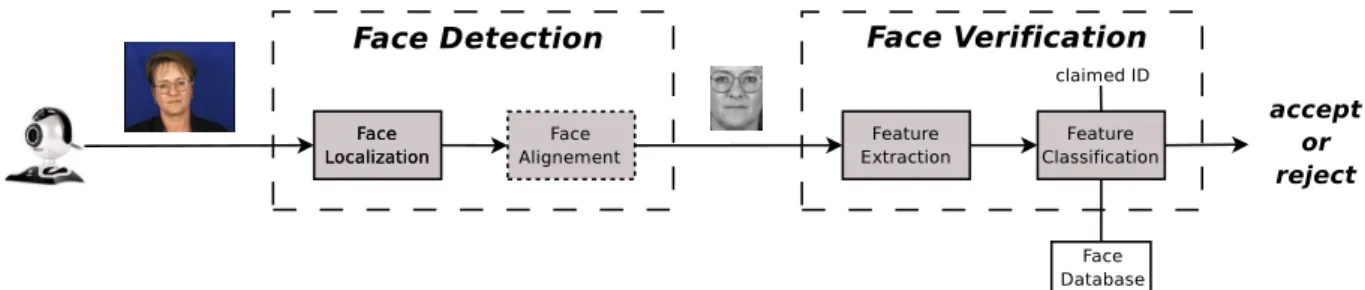
Figure 1.1. Structure of an automatic face verification system, composed of two main modules: face detection and face verification.

An automatic face verification system is composed of two main modules (Fig. 1.1): face detection and face verification. The purpose of the face detection module is to determine whether there are any faces in an image (or video sequence), and if so, to return their position and scale. The term face localization is employed when there is one and only one face in the image. When the localization step only provides a rough segmentation of the face region, a post-processing face alignment step may be required. This step involves locating facial features, such as eyes, nose, mouth or chin, in order to geometrically normalize the face region. Face detection is an important area of research in computer vision, because it serves, as a necessary first step, any face processing system, such as face recognition, face tracking or expression analysis. Most of these techniques assume, in general, that the face region has been perfectly localized. Therefore, their performance significantly depend on the accuracy of the face detection step.

The face verification module consists in two steps: feature extraction and classification. Ideal features should have a discriminant power to differentiate people’s identities and should be robust to intra-class variability, due for instance to illumination, expression changes or slight variation of the pose. Furthermore, as real-time operation is often needed in real-life scenarios, features should be fast to compute. In the classification step, the extracted features (or face representation) is compared to the face model of the claimed identity and the face access is either accepted (client) or rejected (impostor).

(23)

1.2. CHALLENGES 5

1.2

Challenges

Although face detection receives considerable attention, it still remains a difficult pattern recog-nition task, because of the high variability of the face appearance. Faces are non-rigid, dynamic objects with a large diversity in shape, color and texture, due to multiple factors such as head pose, lighting conditions (contrast, shadows), facial expressions, occlusions (glasses) and other facial fea-tures (make-up, beard).

Large variability in face appearance also affects face verification. Furthermore, quoting Moses et al., "the variations between the images of the same face due to illumination and viewing direction are almost always larger than the image variation due to change in face identity" [70]. Another difficulty comes from the lack of reference images to train face templates. In real-life applications, the enrolment procedure has to be fast and is generally done once. The few available training data are usually not enough to cover the intra-personal variability of the face. Moreover a significant mismatch between training and testing conditions may happen (especially lighting). Finally, the verification performance is highly related to the quality of the face localization step.

1.3

Scope and Contributions

This thesis aims to build a fully automatic face verification system which works in real-time. The system must be robust enough to small head pose and lighting variations in order to be used in a real-life low level application such as computer access log-in. Most research has been done in face detection, face alignment and face verification, but few works treat these distinct modules as an ensemble. Most of the papers on face detection do not consider the final application for which the detector is designed and most of the papers on face verification assume a perfect localization of the face, which is not realistic. In this thesis, we consider the automatic face verification as a unified task. The main contributions of this work are briefly presented in the following:

• performance evaluation of face detection systems[80]: several aspects make perfor-mance comparisons very difficult. We underline the importance of a unified face criterion, assessing what is a correctly detected face, when reporting detection rates. We also show how the image scanning process, the overlapped detections merging or even the size of the training

(24)

dataset may affect the performance of a detection system.

• multiview face detection[93]: we propose a novel architecture, based on a pyramid of de-tectors trained for each view. Individual dede-tectors are based on the boosting of Local Binary Pattern (LBP) features. The system works in real-time and shows high performance on bench-mark test sets. Compared to traditional approaches based on Haar-features [105], the detector is more robust to illumination changes and partial occlusion of the face.

• face verification[84]: we propose a new generative approach based on the adaptation of LBP histograms. Generative approaches have proven to be more effective than discriminative ones, mainly because of the lack of training data. Our system shows improved performance compared to other state-of-the-art LBP based techniques.

• face alignment[59]: we extend the Active Shape Model (ASM) [13] method by using an LBP representation instead of pixel intensities. The LBP-ASM system achieves more accurate alignment and is more robust to illumination.

• system-dependent performance measure[82, 83]: we explain that face localization errors may have different impacts depending on the final application. We analyze the effect of the different kinds of localization errors (shift, scale, rotation) on the specific task of face verifi-cation. To properly evaluate the performance of face localization algorithms, we propose to embed the final application (here verification) into the performance measuring process. We empirically demonstrate that the proposed measure gives a better estimate of the quality of the face localization step.

• demonstrators[60]: based on the findings of this thesis, we built several demonstrators, such as a bi-modal (face and speech) biometric demonstrator, a computer access log-in and a face tracking system.

• Torch3vision: it is an open source machine vision library, written insimpleC++, designed for scientific research. It includes standard image processing and feature extraction algorithms and is available from: http://torch3vision.idiap.ch/. All experiments in this thesis have been implemented with Torch3vision.

(25)

1.4. ORGANIZATION OF THE THESIS 7

1.4

Organization of the Thesis

This thesis is organized as follows:

Chapter 2 addresses the problem of frontal face detection. The main previous approaches are reviewed and a method based on boosting LBP features is presented. Special attention is also given to the important issue of performance evaluation. (Papers V, VI)

Chapter 3 extends the frontal face detection system in order to deal with multiview faces. Some recent approaches are reviewed and a novel pyramid architecture is introduced. Experimental analysis is provided for different kinds of head rotations. (Paper X)

Chapter 4 describes a new face verification system based on the adaptation of LBP histograms. Experimental evaluation is provided for both manual and automatic segmentation of the face. (Pa-pers II, VII, IX)

Chapter 5 concerns the performance evaluation of face localization algorithms. It first analyzes the effect of localization errors on the performance of a face verification system. It then presents a new measure which takes into account the performance of the final application. An empirical evaluation is provided for the particular case of face verification. (Papers I, V, VI)

Chapter 6 summarizes the main findings and remarks of the previous chapters and discusses some ideas for future research.

Appendices present additional LBP-based works, respectively on face alignment (Appendix A, Paper VIII), hand posture recognition (Appendix B, Paper IV) and image normalization (Appendix C, Paper III), as well as some demonstrators on face detection and verification (Appendix D).

(26)

(27)

Chapter 2

Frontal Face Detection

Face detection is the first module of the automatic face verification system illustrated in Fig. 1.1. In a verification scenario, we generally assume that the user will cooperate with the system, and thus that the detection module will deal with frontal faces. This is the subject of this chapter.

We first present some previous approaches to the frontal face detection task (Section 2.1). Spe-cial attention is given to boosting-based methods which have been so far the most effective in prac-tice, both in terms of accuracy and speed. One of the main limitations in early boosting-based approaches is the robustness to illumination and partial occlusion of the face. To cope with these limitations, we propose to use Local Binary Pattern (LBP) features (Section 2.2). We also discuss the fundamental problem of evaluating the quality of the face detection step, because its reliability largely affects the performance of the whole verification system (Section 2.3). A detailed description of the experimental setup is then provided (Section 2.4). While not mentioned in the majority of the papers, experiments show that the scanning and overlapped detection merging processes may sig-nificantly influence the accuracy and/or speed of the face detection process (Section 2.5). We finally give some concluding remarks (Section 2.6).

2.1

Related Work

Numerous methods have been proposed to detect faces in images. Many of them are reviewed in two recent survey papers by Yang et al. [111], and by Hjelmas and Low [33]. These methods can be

(28)

organized in two categories: feature-based approaches and appearance-based approaches.

Feature-based approaches make explicit use of face knowledge. They are usually based on the detection of local features of the face, such as the nose, the mouth or the eyes, and the structural relationship between these facial features. Feature-based methods are generally used for face lo-calization (one face) in good quality images. They are robust to illumination conditions, occlusions and viewpoint, but may also be computationnaly expensive.

Appearance-based approaches consider face detection as a two-class pattern recognition prob-lem. They rely on statistical learning methods to build a face/nonface classifier from training sam-ples. These methods are used for multiple face detections in lower image resolutions. Although both classes of methods do not deal with the same problems and environments, appearance-based approaches have recently received considerable attention and have proven to be more successful and robust than feature-based approaches. We will discuss them in more detail hereafter.

2.1.1

Appearance-based Approaches

The concept ofscanning windowis the root idea of appearance-based methods. A sliding window scans the input image at different locations and scales. Each subwindow is then given to a classifier whose goal is to classify the subwindow as eitherfaceornonface. The different appearance-based methods mainly differ in the choice of this classifier. Among the most popular learning classifiers, Support Vector Machines [75, 88, 79], Neural Networks [85, 112], Bayesian classifiers [14] or Hid-den Markov Models [72] have been tried. Some of the most significant approaches are reported below.

Turk and Pentland [101] proposed to perform Principal Component Analysis (PCA) on training face images and to use the eigenvectors, also called eigenfaces, as a face template. A candidate sub-window region is classified according to the distance computed in the PCA subspace after projection. This distance can be interpreted as a measure of faceness.

Sung and Poggio [97] developed a distribution-based system which consists of two steps. First, they partition the face distribution into 6 clusters, approximated by Gaussian functions, and de-compose each cluster in the PCA subspace. The same is done to model the nonface distribution. A distance is then computed between a candidate subwindow and its projection onto the PCA sub-space for each of the 12 clusters. In a second step, a neural network is trained to classify face and

(29)

2.1. RELATED WORK 11 nonfaces based on these distances.

Rowley et al. [85] presented an ensemble of Neural Networks which works on pixel intensities of candidate regions. Each network has a different structure with retinal connections to capture the spatial relationships of pixels (facial features). Detections from individual networks are then merged to provide the final classification decision.

Féraud et al. [19] proposed another Neural Network model, based on the Constrained Gen-erative Model (CGM). CGMs are auto-associative connected Multi-Layer Perceptrons (MLP) with three large layers of weights, trained to perform a non-linear PCA. Classification is obtained by considering the reconstruction errors of the CGMs.

One of the most accurate face detector was reported by Roth et. al [112] who use the Sparse Net-work of Winnows (SNoW) learning architecture. SNoW is a single layer Neural NetNet-work, composed of linear threshold units, that uses the Littlestone’s Winnow update rule [50]. Their system uses boolean features that encode the positions and intensity of pixels. A comparative analysis of SNoW with Neural Networks and Support Vector Machines (SVM) can be found in [113] and [18].

Appearance-based methods reported above provide accurate detection results with few false alarms. However, all of them need several seconds at best to process an image, mainly because candidate subwindows need to be geometrically and photometrically normalized before classifica-tion. This limitation is restrictive for real-life applications that need real-time face detection (>15

frames per second).

In 2001, Viola and Jones [105] introduced the first real-time frontal face detection system. In-stead of using pixel information, they proposed to use a new image representation and a set of simple features that can be computed at any position and scale in constant time. Boosting learning is both used for feature selection and classifier design. [105] is the first work of a new family of face detection methods, called boosting-based methods, which we will describe in more details in the next section.

(30)

2.1.2

Boosting-based Approaches

Boosting learning

Recently, most of the attention has been paid to boosting-based approaches since the famous work of Viola and Jones [105]. These approaches show very good results both in terms of accuracy and speed, and are then well suited for real-time applications. The Viola and Jones face detector is presented in more details in this section because a lot of recent work has concentrated on improving this detector and because it will serve as a baseline comparison system in our experiments.

A complete introduction to the theoretical basis of boosting and its applications can be found in [65]. The underlying idea of boosting is to linearly combine simple classifiers hj(X)to build a

strong ensembleH(X): H(X) = n X j=1 wjhj(X). (2.1)

The selection of the weak classifiershj(X)as well as the estimation of the weightswj are learned

by the boosting procedure. Each classifierhj(X)aims to minimize the classification training error

on a particular distribution of the training samples. At each iteration (i.e. for each weak classifier), the boosting procedure updates the weight of each sample such that the misclassified ones get more weight in the next iteration. Boosting hence focuses on the examples that are hard to classify. Several variants of Boosting exist. They mainly differ in the iterative reweigting process of the training samples.AdaBoost[20] is probably the most well known.

Haar-like feature classifiers

In 2001, Pavlovic and Garg [77] proposed to boost pixel-based classifiers for face detection. Instead of directly using pixel information, Viola and Jones introduce a set of simple features (Fig. 2.1), derived from Haar wavelets. A feature is computed by summing the pixels in the white region and

(31)

2.1. RELATED WORK 13 subtracting those in the dark region. Haar-like features can be computed efficiently with the

inte-gral imagerepresentation orsummed area table, first introduced by Crow [16] for texture mapping.

At a given location(x;y)in an image, the value of theintegral imageii(x;y)is the sum of the pixels above and to the left of(x;y):

ii(x;y) = X

x0_≤x,y0_≤y

i(x0;y0),

wherei(x0_;_y0₎_{is the pixel value of the original image at location}₍_x0_;_y0₎_{. If}_s₍_x_;_y₎_{is the cumulative}

row sum, withs(x;−1) = 0ands(−1;y) = 0, theintegral imagecan be computed in one pass over the original image using the following pair of recurrences:

s(x;y) = s(x;y−1) +i(x;y), (2.2)

ii(x;y) = ii(x−1;y) +s(x;y). (2.3)

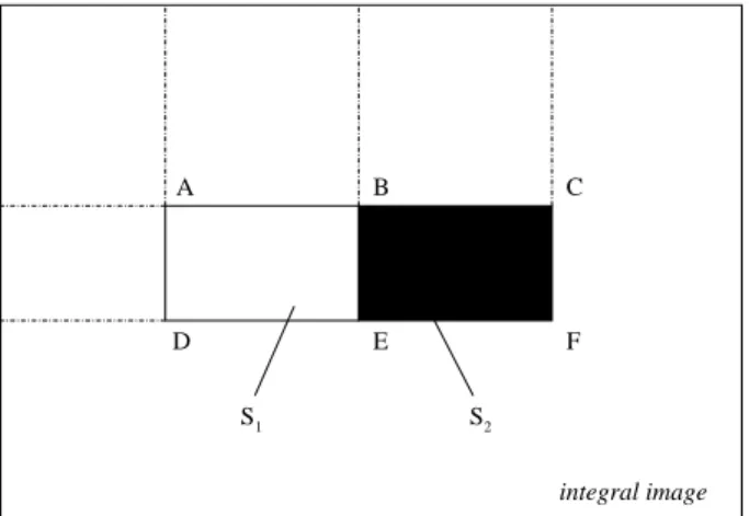
An example is given in Fig. 2.2. To compute the illustrated feature, only 6 table accesses and 7 simple operations are needed. Haar-like features can then be computed very quickly at any scale and position in constant time.

B A D E F C S1 S2 integral image

Figure 2.2.Haar-like feature computation with the integral image. The feature value is:S1−S2, withS1=E−B−D+A

andS2=F−C−E+B

The feature set is obtained by varying the size and position of each type of Haar-like features. To select the weak classifiershj(X)of Eq. 2.1, the learning procedure works as follows. Each candidate

(32)

The weak classifier then determines the optimal threshold θi which minimizes the classification

error. The task of the learning procedure is to find the featuref such that the minimum number of samples are misclassified. A weak classifierhj(X)thus consists of a Haar-like featuref, a threshold θand a paritypindicating the direction of the inequality:

hj(X) =      1 ifpf(X)< pθ, 0 otherwise. (2.4)

Such classifier can be seen as a single-node decision tree, also calleddecision stump.

Cascade architecture

Considering a set of images, thedetection rateof a face detector is defined as the number of correctly detected faces over the total number of faces in the test set. Afalse alarmis accounted each time the system badly classifies a background region as a face. A higher detection rate (with less false alarms) can be achieved by increasing the numbernof weak classifiershj(X)of the ensembleH(X)

of Eq. 2.1 . On the other hand, increasingnwill also increase the complexity of the ensemble and then the computation time.

To deal with the trade-off performance vs. computation time, Viola and Jones propose a cascade structure of ensembles. This framework is motivated by the nature of the problem which is a rare event detection problem. In an image, only a very small number of subwindows contain a face (generally<0.1%). 2

τ

> >

τ

_M 1

τ

< <

τ

₂ <

τ

_M 1

τ

> M

H (x)

reject subwindow (Non Face)

Face

all candidate

subwindows

H (x)

1

H (x)

2

Figure 2.3. Overview of the cascade architecture which works as a degenerated decision tree. At each stage, the classifier either rejects the sample and the process stops, or accepts it and the sample is forwarded to the next stage.

(33)

2.1. RELATED WORK 15 The cascade, illustrated in Fig. 2.3, works as follows: Each ensembleHi(X)is designed to detect

almost all faces (>99%) while rejecting as much background regions as possible. This is done by adjusting the thresholds τi on a validation set. The first ensemble H1(X), composed of only two

features, rejects approximately 50% of the background subwindows. As the task becomes more difficult, the next ensembles contain more weak classifiers. With such a simple-to-complex ap-proach, most of the background regions are quickly discarded early in the cascade and only face subwindows should pass over all the cascade. Viola and Jones compare a cascade of ten 20-feature classifiers with a monolithic 200-feature classier. They report that the accuracy of both classifiers is not significantly different, but that the cascade version performs almost 10 times faster.

2.1.3

Discussion

Since the work of Viola and Jones [105] published in 2001, most of the research in face detection has focused on the improvement of their cascade architecture. Related works can be classified in three directions, whether they provide alternative feature set, boosting algorithm or architecture design.

Alternative boosting algorithms

At each iteration, AdaBoost selects the weak classifier which minimizes the (weighted) classification error, regardless if the error is a false positive or false negative. The goal of the detection cascade is however to achieve high detection rates (>99%) with moderate false alarm rates (>50%) for each stage. In [106], Viola and Jones proposed a modified version of the original boosting algorithm, called Asymmetric AdaBoost, which gives more weight to the positive examples. A very similar cost-sensitive algorithm,CS-AdaBoost, has been published by Ma and Ding [56].

Wu et al. [108] also observed that AdaBoost is an indirect way to meet the learning goals of the cascade. They proposed a cascade learning procedure based on direct forward feature selection which is much faster than AdaBoost while yielding similar performance. McCane and Novins [64] also proposed an alternative to boosting. They explained that since the feature set is parame-terizable (size and position of the Haar-like masks), the feature selection is a form of numerical optimization, and they provided a fast (300-fold) heuristic to find (suboptimal) features.

(34)

and showed that the latter performs slightly better. However, according to [9], the choice of the boosting algorithm has more impact on the speed of the detector than on classification performance. Li et al. [46] proposed a new boosting algorithm, called FloatBoost, to solve the monotonicity problem encountered in the sequential forward search procedure of AdaBoost. After each iteration,

FloatBoost removes the least significant weak classifier which leads to a higher error rate of the

global classifier. Compared to the sequential AdaBoost, FloatBoost needs fewer weak classifiers to achieve the same error rate. The cost of such improvement is a learning time of about 5 times longer.

Other variants of AdaBoost have been tried for face detection, like Kullback-Leibler Boost-ing[51],LogitBoost[21],Jensen-Shannon Boosting[37],Vector Boosting[34] orMRC-Boosting[110]

Alternative feature sets

Lienhart et al. [49] proposed an extended set of Haar-like features, including45◦ _{rotated features}

(Fig. 2.4). To compute these features, they described a fast calculation scheme for rotated rectangles, which is very similar to the integral image. At a given detection rate, the authors reported a 10% false alarm (non-face regions classified as being faces) improvement with this extended features set. Li and Zhang [46] also extended the original Haar-like feature set by including features with non-adjacent regions (Fig.2.5).

Figure 2.4.Extended Haar-like feature set used by Lienhart et al. [49].

dx dy dx’ x y dx dy y x dx’ dx dy y x

Figure 2.5.Extended Haar-like feature set used by Li et al. [46].

Zhang et al. remarked in [115] that in the last stages of the cascade, the nonface examples collected by bootstrapping become very similar to face examples and that weak classifiers based on local Haar-like features reach their limit. Instead, they proposed to switch to a global representa-tion of the face and boost PCA coefficients.

(35)

2.1. RELATED WORK 17 Mita et al. [68] proposed new features based on co-occurrence of multiple Haar-like features, called joint Haar-like features, which capture the structural similarities within the face class. Given the same number of features, they reported improved performance compared to the original system. In [22], Fröba and Ernst used a Modified version of the Census Transform (MCT) to build weak classifiers, while Hadid et al. [29], Jin et al. [40] or Zhang et al. [117] chose LBP features (cf. Section 2.2.1).

Alternative cascade architecture

The two main limitations of the detector of Viola and Jones [105] are a long training procedure and the choice of the cascade parameters. A lot of effort has been given on finding training alternatives, but much less attention has been paid to the fundamental problem of the cascade architecture design.

In [54], Luo published a method to adjust the stage thresholds after the training of the cascade. He reported improved performance compared to the original Viola and Jones detector. However, his post-processing technique does not help to chose the threshold values during training and then does not solve the problem of when to stop training the current stage and go for the next one.

McCane and Novins [64] pointed out that the root idea of the cascade architecture is to quickly discard nonface subwindows. Since there are much less faces than nonfaces regions, the speed of the detector can be seen as the average speed to reject a nonface subwindow. McCane and Novins argued that the speed of the detector is the function to minimize and proposed a method to deter-mine the optimal cascade speed.

Grossman [28] first trained a single-stage classifier with AdaBoost. Using dynamic program-ming, he then partitioned the weak classifiers of this single stage to build a cascade of optimal speed with almost identical behavior to the original single-stage classifier. The main drawback of Grossman’s method is to produce more false alarms, because it does not take advantage of the bootstrapping technique of the original cascade training approach.

Li and Satoh [45] proposed to sequentially combine a classical boosted cascade with a cascade of three SVM classifiers, trained with the features selected by AdaBoost in the last stage of the classical cascade.

(36)

clas-sifiers instead of simple decision stumps (Eq. 2.1). They reported improved results for the same computation time.

Wu et al. [107] described a nested cascade structure. The difference with the classical cascade approach is that each layer is used as the first weak classifier of the following layer, thus retaining the discriminative power of previous layers (confidence of the predecessor). A similar approach was proposed by Xiao et al. [109].

Brubaker et al. [9] introduced a new criterion for cascade training to select stage thresholds (balance between detection and false alarm rates) and number of weak classifiers (when to stop training in one stage and move on to the next one), based on a probabilistic model of the overall cas-cade’s performance. They also evaluated several feature selection methods to speed up the training process and investigated CART as weak classifiers.

2.2

Frontal Face Detection Using Local Binary Patterns

The face detection algorithm introduced in this section is an extension of Viola and Jones sys-tem [105] based on boosted cascades of Haar-like features. As pointed out by Zhang et al. [115], these features are very efficient early in the cascade to quickly discard most of the background regions. However, in the last stages of the cascade, a large number of Haar-like features (several hundreds) are necessary to reach the desired detection/false acceptance rate trade-off. It results in a long training procedure and cascades with several dozens of stages which are difficult to design. Furthermore, Haar-like features are not robust to local illumination changes.

To cope with the limitation of Haar-like features, we propose to use LBP features (Section 2.2.1). The method to build the weak classifiers is inspired by the work of Fröba and Ernst [22] and the cascade training is done with AdaBoost [20] (Section 2.2.2).

2.2.1

LBP Features

The LBP operator is a non-parametric 3x3 kernel which summarizes the local spacial structure of an image. It was first introduced by Ojala et al. [73] who showed the high discriminative power of this operator for texture classification. At a given pixel position(xc, yc), LBP is defined as an ordered

(37)

2.2. FRONTAL FACE DETECTION USING LOCAL BINARY PATTERNS 19 83 75 126 99 95 141 91 91 100 0 0 0 1 0 1 1 1 binary: 00111001 decimal: 57 comparison

with the center binary intensity

Figure 2.6.The basic Local Binary Pattern (LBP) operator.

pixels (Fig. 2.6). The decimal form of the resulting 8-bit word (LBP code) can be expressed as follows: LBP(xc, yc) = 7 X n=0 s(in−ic)2n, (2.5)

where ic corresponds to the grey value of the center pixel (xc, yc), in to the grey values of the 8

surrounding pixels, and functionsis defined as:

s(x) =      1 if x>0, 0 if x <0. (2.6)

Note that each bit of the LBP code has the same significance level and that two successive bit values may have a totally different meaning. Actually, The LBP code may be interpreted as a kernel structure index. By definition, the LBP operator is unaffected by any monotonic gray-scale transformation which preserves the pixel intensity order in a local neighborhood (Fig. 2.7).

Later, Ojala et al. [74] extended their original LBP operator to a circular neighborhood of dif-ferent radius size. Their LBPP,R notation refers toP equally spaced pixels on a circle of radius

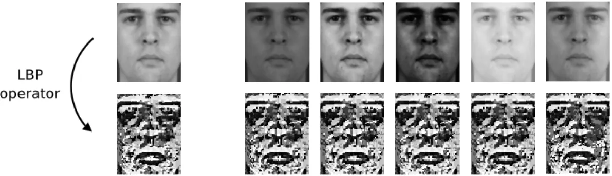
Figure 2.7. LBP robustness to monotonic gray-scale transformations. On the first row, the original image (left) as well as several images (right) obtained by varying the brightness, contrast and illumination. The second row depicts the corresponding LBP images which are almost identical.

(38)

R. In [74], they also noticed that most of the texture information was contained in a small subset of LBP patterns. These patterns, called uniform patterns, contain at most two bitwise 0 to 1 or 1 to 0 transitions (circular binary code). 11111111, 00000110 or 10000111 are examples of uniform patterns. They mainly represent primitive micro-features such as lines, edges, corners. LBPu2

P,R

denotes the extended LBP operator (u2for only uniform patterns, labelling all remaining patterns with a single label). TheLBP8,2operator is illustrated in Fig. 2.8.

Figure 2.8. The extended LBP operator with (8,2) neighborhood. Pixel values are interpolated for points which are not in the center of a pixel.

Recently, new variants of LBP have appeared. For instance, Jin et al. [40] remarked that LBP features miss the local structure under some certain circumstance, and thus they introduced the

ImprovedLocal Binary Pattern (ILBP). Huang et al. [38] pointed out that LBP can only reflect the

first derivation information of images, but could not present the velocity of local variation. To solve this problem, they proposed anExtendedversion of Local Binary Patterns (ELBP).

Due to its texture discriminative property and its very low computational cost, LBP is becom-ing very popular in pattern recognition. Recently, LBP has been applied for instance to face de-tection [40], face recognition [116, 1], image retrieval [98], motion dede-tection [31], visual inspec-tion [102], hand posture recogniinspec-tion [43] (see Appendix B) or image normalizainspec-tion [43]1 _(see

Ap-pendix C). We finally point out that, approximately in the same time the original LBP operator was introduced by Ojala [73], Zabih and Woodfill [114] proposed a very similar local structure fea-ture. This feature, calledCensus Transform, also maps the local neighborhood surrounding a pixel. With respect to LBP, theCensus Transform only differs by the order of the bit string. Later, the

Census Transformhas been extended to become theModified Census Transform(MCT) [22] which

takes into account the center pixel in the bit string and compares to the average intensity value within the neighborhood. Again, one can point out the same similarity between ILBP and MCT (also published at the same time).

1_a _more _exhaustive _list _of _applications _can _be _found _on _Oulu _University _web _site _at: http://www.ee.oulu.fi/research/imag/texture/lbp/lbp.php

(39)

2.2. FRONTAL FACE DETECTION USING LOCAL BINARY PATTERNS 21 In this chapter, we will consider the ILBP version (or MCT), described in [40] (or in [22]), which outputs a 9-bit word (ILBP code). In the rest of this chapter, we will use theLBPnotation to refer to ILBP (or MCT) features.

2.2.2

Weak Classifiers and Cascade Training

Weak classifiers

A weak classifierhp(x)consists of a look-up table of29−1 = 511bins2, which is the total number

of possible LBP codesx, and is associated to a specific pixel locationp. Each bin of the look-up table contains a real value which corresponds to the weight of the related LBP code. In a test image, at a given locationp, the output of classifierhp(x)is the value of the binx, wherexis the LBP code

computed at locationp. LetHn(X)be the ensemble classifier of stagen:

Hn(X) =

X

p∈Wn

hp(x), (2.7)

where Wn is the set of pixel locations for stagen. Fig. 2.9 illustrates a stage ensemble of 5 weak

classifiers, as well as the look-up table for one of them.

Figure 2.9.Pixel classifier (left) and its associated look-up table (right).

Cascade training

In the AdaBoost framework, the algorithm selects the weak classifier which minimizes the clas-sification error rate on a weighted distribution of positive and negative samples. Here, a weak classifier consists of a look-up table associated to a pixel location. Then, AdaBoost aims to select

(40)

pixel locations and to build the associated look-up tables. The training algorithm is detailed in [22] and is explained below.

At each stagenof the cascade, the numberPn of weak classifiers is fixed, as well as the number Tnof boosting iterations. Pn is then the size of the set of pixel locationsWn.

At each boosting iteration t, to select the best pixel classifier, two look-up tables Lf ace

p and

Lnonf ace

p are allocated for each pixel location of Wn. Then, for each locationp, the LBP operator

is applied on a training set of face samples. For each sample, the computed LBP code is used to identify the bin ofLf ace

p , which is increased by an amount equal to the weight of the sample. The

same is done with a training set of nonfaces to populate theLnonf ace

p tables. The classification error at positionpis given by:

p= 511

X

j=1

min(Lf acep [j], Lnonf acep [j]). (2.8)

The look-up tableLp∗ of the selected pixel classifier at iterationtis then computed for each binj:

Lp∗[j] =      1 ifLf ace p [j]> Lnonf acep [j], 0 otherwise. (2.9)

A pixel classifier thus consists of a look-up table of 0s and 1s. During the boosting learning, a discriminative pixel location may be selected several times. At the end of the boosting procedure, look-up tables associated to the same pixel location are merged into a single table. For each bin, a weighted (by coefficientwtof AdaBoost, Eq. 2.1) sum is done on the bin values of each table. Weak

classifiershp(x)of Eq. 2.7 consist of these single weighted look-up tables.

Note that this boosted cascade of LBP framework has been successfully applied to the task of hand posture recognition [43] and described in Appendix B.

(41)

2.3. PERFORMANCE EVALUATION 23

2.3

Performance Evaluation

2.3.1

Performance Measure

On a given test database, the performance of a face detection system is measured in terms of De-tection Rate (DR), which is the proportion of faces detected, and the number of False Acceptances (nFA), which is the number of background regions badly classified as face regions. DR and nFA are related. Increasing (resp. decreasing) DR usually means increasing (resp. decreasing) nFA as well. Then, instead of providing a single operating point, it is more appropriate to provide the Free Receiver Operator Characteristic (FROC) curve, which plots DR versus nFA. The ROC curve is very similar. It represents the detection rate versus the false acceptance rate. However, the ROC curve is not adapted for face detection because the false acceptance rate, which is defined as the number of false acceptances over the total number of scanned windows containing no face, depends on the scanning process.

2.3.2

Face Criterion

Reporting detection and error rates is not enough to allow fair performance comparisons. The way detections and errors are accounted should also be clearly described. In other words, a face criterion, assessing what is a correctly detected face, should be defined. Fig. 2.10 illustrates the problem. Some people will account five correct face detections, while other people, using a more restrictive face criterion, will only report the detection on the left. Recently, Jesorsky et al. [39] introduced a relative error measure based on the distance between the detected and the expected (ground-truth) eye center positions. Let Cl (respectivelyCr) be the true left (resp. right) eye coordinate position

and letC˜l(resp. C˜r) be the left (resp. right) eye position estimated by the face detection algorithm.

(42)

This measure can be written as:

deye=

max(d(Cl,C˜l), d(Cr,C˜r)) d(Cl, Cr)

(2.10)

where d(a, b) is the Euclidean distance between positions a and b. A successful detection is ac-counted if deye < 0.25, which corresponds approximately to half the width of an eye. This is, to

the best of our knowledge, the first attempt to provide a unified face localization measure. This fundamental problem of face criterion is analyzed in Chapter 5.

2.3.3

Application-dependent Evaluation

The performance evaluation should depend on the purpose of the detector. The balance between detection rate, number of false acceptances and speed should be properly weighted. If the detector is used for face recognition, the detection rate must be maximized, to the detriment of the number of false acceptance which will be rejected by the recognition process. On the other hand, if the detector is used for active tracking in video conferencing, accuracy may need to be sacrificed for speed. One may use temporal information to refine the accuracy and remove false acceptances. A clear description of the scenario (final application) and of the evaluation protocol (DR, nFA, speed) is needed when assessing the performance of face detection systems.

2.4

Experimental Setup

2.4.1

Training Data

Appearance-based face detection methods highly rely on the training sets to find a discriminant function between face and nonface classes. Robustness to appearance variability of the face is achieved by incorporating this variability into the training set. For instance, to detect the face of people wearing glasses, several samples of faces with glasses are added into the face training set. We proceed similarly to deal with small pose variations of the head, facial expressions, people gen-der, aging and so on. Actually, the richness of the training set is fundamental for the performance of the face detector system.

(43)

2.4. EXPERIMENTAL SETUP 25

Faces

Many face databases are available on the Internet. Among them, we selected face images from BANCA [3] (Spanish corpus), Essex3_{, Feret [78], ORL [89], Stirling}4_{and Yale [6] databases. The}

extraction of each face is done as follows:

1. Each face is labelled by manually locating the center position of both eyes. These two land-mark points (groundtruth) are used to geometrically align the faces.

2. Face/head anthropometric measures are used to determine the face bounding box and crop the face region. The widthbbxwof this region (in pixels) is defined by:

bbxw=

zy_zy

2∗pupil_se∗dGT (2.11)

wheredGT is the distance (in pixels) between both eye centers, andzy_zy= 139.1(mean width

of a human face in [mm]) andpupile_se = 33.4 (half of the inter-pupil distance in [mm]) are anthropometric constants given by Farkas in [17]. According to Fig 2.11 and giveny_up =

pupile_se, the position of the bounding box can be computed.

3. The cropped face is then subsampled to the size of 19x19 pixels. This template size was also used by Sung et al. [97], Papageorgiou et al. [76] or Osuna et al. [75], while Rowley [85] chose a template of 20x20 and Viola and Jones [105] a template of 24x24. In his thesis [15], Cristinacce showed that the choice of an optimal face template size is not trivial. The set of faces is then split in two sets of equal size (training and validation).

The concept of scanning window is a discrete process. Due to time constraints, a test image can not be scanned at each position and scale. To detect faces which do not exactly fit the scanning window, small localization errors are artificially generated by slightly shifting, scaling and rotating the original face. Training and validation sets can be further extended by mirroring each face example (Fig. 2.12). From each original face image, 10 virtual samples are randomly created.

3_{images available from: http://cswww.essex.ac.uk/mv/allfaces/index.html} 4_{images available from: http://pics.psych.stir.ac.uk/}

(44)

face bounding box eye center coordinates

2 * pupil_se zy_zy

y_up

(square)

Figure 2.11.Face bounding box determined by face anthropometric measures defined in [17].

Figure 2.12.Virtual face training examples (right), created from the original cropped face (left).

Nonfaces

Several hundreds of images containing no face have been collected on the Internet. Scanning these images at different positions and scales provide potentially billions of nonface examples. Again, variability of the training set is crucial for the classifier to appropriately estimate the decision boundary. However, in the nonface case, it is not easy to define what is a nonface and choose relevant examples (i.e. close to the face/nonface boundary). We also considered face images and extracted multiple subwindows containing small parts of face regions. Some examples are shown in Fig. 2.13.

(45)

2.4. EXPERIMENTAL SETUP 27

Figure 2.13.Nonface training examples.

Figure 2.14.Image examples of the XM2VTS database (standard set).

2.4.2

Benchmark Test Sets

XM2VTS database

The XM2VTS database [55] has been designed for multi-modal biometric authentication. It con-tains synchronized image and speech data recorded on 295 subjects during four sessions taken at one month intervals. Two shots were recorded per session, resulting in 2360 images. These images represent the XM2VTS standard set. Each color image of size 720x576 contains one person on a uniform blue background and in controlled lighting conditions (Fig. 2.14). For each of the 295 iden-tities, 4 extra shots have been acquired with left/right side directional lighting. This set of 1180 images is calleddarkened set. Fig. 2.15 shows some examples.

(46)

Figure 2.16.Image examples of the BioID database.

BioID database

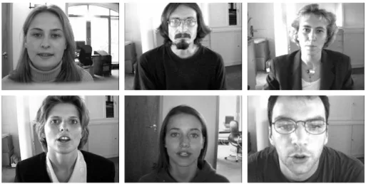
The BioID database [39] has been recorded to test face detection algorithms onreal worldconditions (variation in illumination, background and face size). The dataset consists of 1521 gray level images of 23 individuals with a resolution of 384x286 pixel (Fig. 2.16).

Purdue AR database

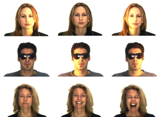
The Purdue AR database [63] contains over 3000 color images of 126 people taken in controlled lightning and background conditions. This database has been created to test face recognition algo-rithms under several mixed factors: facial expressions (neutral, smile, anger and scream), illumi-nation (left, right and both side light on) and occlusion (wearing glasses and scarf). Some examples are given in Fig. 2.17.

2.4.3

Image Scanning

To detect faces in an image, the face detector (i.e. the face/nonface classifier) scans the image at multiple locations and scales. At each position, the subwindow is evaluated by the detector and is classified as either a face or a nonface with a certain confidence. The scanning window process is the root idea of the detection system.

(47)

2.4. EXPERIMENTAL SETUP 29

Figure 2.17.Image examples of the Purdue database.

Scanning parameters

The choice of the scanning parameters has a direct impact on the number of subwindows to be classified, and thus on the computation time. Let us introduceSW the size of the scanning window,

SWf acemodel the size of the face template (i.e. smallest possible value ofSW), ands = _SW_{f acemodel}SWi

the scale of the scanning window. These scanning parameters are then defined as:

• SWmin, SWmax: the min/max sizes (in pixels) of the scanning window, with SWf acemodel ≤ SWmin≤SWmax≤min(Imagewidth, Imageheight)

• ds: the scale factor (ratio between two consecutive scales)

• dx,dy: the horizontal/vertical shift steps (in pixels)

The scanning process starts with a scanning window of sizeSWmin. The subwindow is horizontally

(resp. vertically) shifted in the image by[s·dx](resp. [s·dy]), where[]is the rounding operator and

s= SWmin

SWf acemodel is the scale. The scanning window is then scaled to a size ofSWmin·dsand shifted

(48)

Two types of scanning

Scaling can be achieved in two different ways:

1. the image is iteratively subsampled, while the size of the scanning window is kept constant. This method is referred to aspyramidscanning.

2. the scanning window is resized for each scale level, rather than subsampling the image. We refer to this method asmultiscalescanning.

When the computation cost to classify a subwindow does not depend on the size of the subwindow (scale invariant), the multiscale mode is much faster, because no image subsampling nor subwin-dow cropping is needed. Features based on summed area of pixels, like Haar-like or LBP features, can be computed in constant time at different scales with the integral image representation. Those features are then candidates for multiscale scanning. On the other hand, features based on inde-pendent pixel values can not take advantage of this scanning method (the pixel interpolation cost is scale dependent). In this work, we will only usemultiscalescanning.

2.4.4

Merging Overlapped Detections

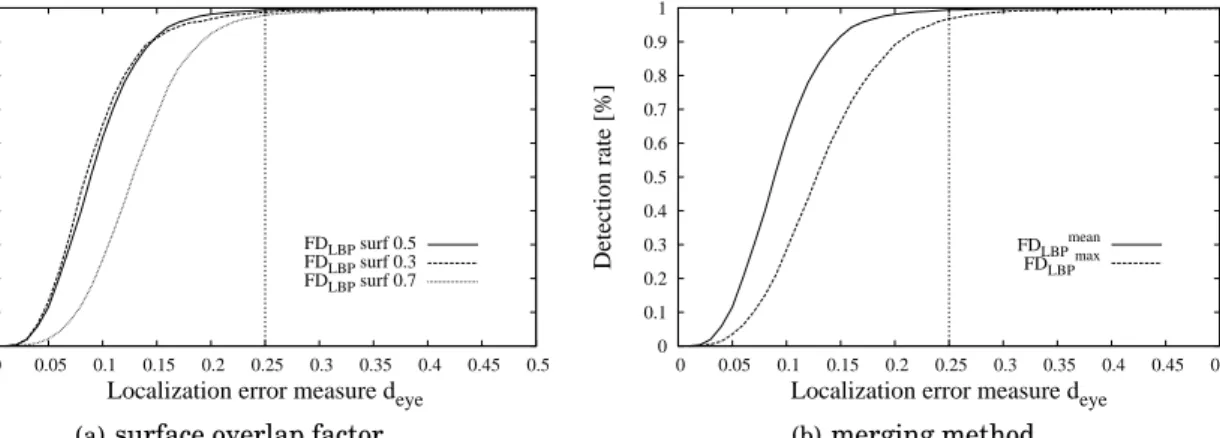
Multiple detections at different locations and scales may occur around a face in the image, because the face classifier is trained to be insensitive to small localization errors. The same behavior may happen around a background region. However, overlapped false alarms usually appear with less consistency than true detections. This assumption is useful to reduce the number of false alarms and to combine true detections, as illustrated in Fig. 2.18. The image on the left shows a scanned image with multiple detections around the face and some false alarms in the background. In the image on the right, false alarms have been removed and the detections around the face have been merged. After the image scanning, the processing of the multiple detections consists in two steps:

1. clustering: two detections belong to the same cluster if the detected regions overlap by a given percentageφ. A cluster is a candidate for merging (next step) if the number of detec-tions (or sum of confidence detection) is above a given threshold η. Another variant could consider the aggregate confidence score (output of the classifier) of the detections instead of their occurrence. If a cluster is not candidate, all detections of this cluster are removed.

(49)

2.4. EXPERIMENTAL SETUP 31

Figure 2.18.Merging of multiple detections (isolated detections are removed).

2. merging: various heuristics exist to combine multiple detections of a cluster. The simplest one selects the detection with the highest confidence score. However, a more precise face localization is obtained by averaging the bounding boxes of each detected region (upper left and down right positions). Again, each bounding box could also be weighted by its confidence score.

Parametersφandηare not easy to choose. Ifφis too small, overlapped detections of the same cluster may be separated, while ifφis too large, two close clusters may merge (ex: partially occluded faces in a crowd). Similarly, If η is too small, overlapped false alarms may be considered as a candidate cluster, while ifηis too large, true candidate clusters may be discarded (balance between detection rate and false alarms). Furthermore, η is related to the choice of scanning parameters, because the finer the scanning, the larger the number of detections. The design of an efficient clustering/merging module is therefore not trivial and may significantly affect the performance of the face detector system in terms of detection rate and number of false alarms (clustering), and of detection accuracy (merging).

2.4.5

Benchmark Face Detectors

FDLBP face detector

This face detector is based on the boosting of LBP features and is described in Section 2.2. The baseline system is composed of 3 stages of respectively 5, 10, and 50 classifiers (empirically chosen), trained with respectively 50, 100, and 300 boosting iterations (following [22] using a training set

(50)

and a validation set of ∼50.000 faces. The decision threshold of each stage has been chosen on the face validation set to achieve 99% detection rate. On a 3GHz Pentium 4 with 1Go RAM, the training of the whole cascade lasts around 5 hours. The scanning and overlap merging parameters were chosen as follows:

• step x factor:dx= 0.05(corresponds to a shift of 1 pixel for a bounding box of size19×19)

• step y factor:dy= 0.10(empirically chosen twice the step x factor)

• scale factor:ds= 1.125(according to [105])

• min scanning window size: depends on the experiment

• min scanning window size:SWmax= size of the image

• surface overlap factor:φ= 0.5(empirically chosen; depends on the step factors)

• detection confidence threshold:η= 1.5

FDHaar face detector

We use the face detector included in the OpenCV library available at: http://sourceforge. net/projects/opencvlibrary/. The detector has been implemented by Lienhart and is related to his paper [49]. We chose the model called alt tree. The 47-stage cascade is composed of 8468 Haar-like stump classifiers. We have no information on the training of the model (training set size, threshold selection, face model, training duration, ..). Because the system only outputs bounding boxes, we empirically estimated the coordinates of the eyes from the boxes by running the detector on a set of simple face images and computing the average detected face image.

2.5

Frontal Face Detection Results

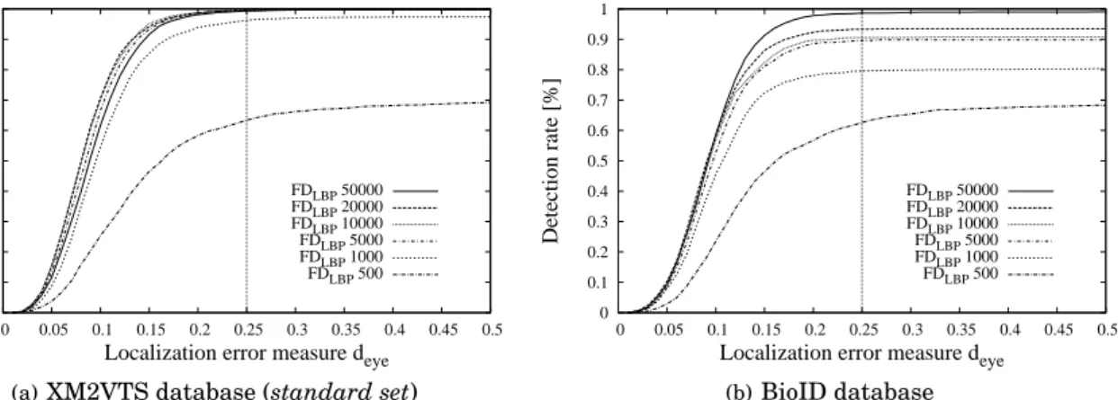
In this Section, face detection experiments will be done in localization mode (only one face per image). For each detector, we only consider the detection with the highest confidence score. In order to assess the localization accuracy of a system, cumulative distributions of Jesorsky’sdeyemetric are

(51)

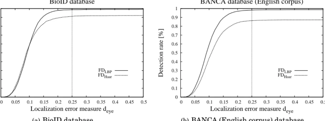
2.5. FRONTAL FACE DETECTION RESULTS 33 detectors in several conditions: controlled (XM2VTSstandard set), uncontrolled lighting (XM2VTS

darkened set), realistic office scenario (BioID), facial occlusions and expression variation (Purdue),

uncontrolled environment (BANCA English). In a second set of experiments, we will only consider FDLBP and show the effect of several parameters such as scanning or merging parameters, which may affect detection performance, both in terms of accuracy and speed.

In the following experiments, we will consider that system A is significantly better than system B, when system A will give statistically better results than system B with a confidence level of 99%, with a standard proportion test, assuming a binomial distribution for the errors, and using a normal approximation.

2.5.1

LBP vs. Haar Face Localization Results

Evaluation on the XM2VTS database (standard set₎

Thedeyecumulative distributions were collected forF DLBP andF DHaarface detectors. The XM2VTS

database has been recorded in well controlled conditions (uniform background and frontal lighting). Both systems are supposed to give similar performance. Fig. 2.19(a) confirms this assumption. For

deye≤0.255,F DLBP achieves99.5%detection rate compared to97.7%forF DHaar.

Evaluation on the XM2VTS database (darkened set₎

The XM2VTSdarkened setset has been recorded with the same setup than thestandard set, but with directional lighting respectively illuminating the left and the right side of the face. We ex-pect that the resulting shadows on the face should more affect theF DHaar system, because of the

sensitivity to local variations of pixel values. However, Fig. 2.19(b) shows that both systems are similarly affe