https://doi.org/10.17576/jkukm-2020-32(1)-11
Optimizing Hopfield Neural Network for Super-Resolution Mapping
Anuar M. Muad*, Siti Khadijah Mohd. Zaki and Sarah Abbood JasimCenter for Integrated Systems Engineering and Advanced Technologies (INTEGRA), Faculty of Engineering & Built Environment, Universiti Kebangsaan Malaysia, Malaysia
*Corresponding author; email: [email protected] Received 27 February 2019, Received in revised form 12 June 2019
Accepted 16 September 2019, Available online 28 February 2020
ABSTRACT
Remote sensing is a potential source of information of land covers on the surface of the Earth. Different types of remote sensing images offer different spatial resolution quality. High resolution images contain rich information, but they are expensive, while low resolution image are less detail but they are cheap. Super-resolution mapping (SRM) technique is used
to enhance the spatial resolution of the low resolution image in order to produce land cover mapping with high accuracy. The mapping technique is crucial to differentiate land cover classes. Hopfield neural network (HNN) is a popular approach
in SRM. Currently, numerical implementation of HNN uses ordinary differential equation (ODE) calculated with traditional
Euler method. Although producing satisfactory accuracy, Euler method is considered slow especially when dealing with large data like remote sensing image. Therefore, in this paper several advanced numerical methods are applied to the formulation of the ODE in SRM in order to speed up the iterative procedure of SRM. These methods are an improved Euler,
Runge-Kutta, and Adams-Moulton. Four classes of land covers such as vegetation, water bodies, roads, and buildings are used in this work. Results of traditional Euler produces mapping accuracy of 85.18% computed in 1000 iterations within 220-1020 seconds. Improved Euler method produces accuracy of 86.63% computed in a range of 60-620 iterations within 20-500 seconds. Runge-Kutta method produces accuracy of 86.63% computed in a range of 70-600 iterations within 20-400 seconds. Adams-Moulton method produces accuracy of 86.64% in a range of 40-320 iterations within 10-150 seconds. Keywords: Euler; optimization; ordinary differential equation; remote sensing; super-resolution mapping
ABSTRAK
Penderiaan jauh merupakan suatu sumber maklumat berkenaan tentang litupan tanah di atas permukaan bumi. Pelbagai jenis imej penderiaan jauh menawarkan kualiti resolusi spatial yang berbeza. Imej dengan resolusi tinggi mengandungi maklumat yang banyak tetapi harganya mahal, manakala imej dengan resolusi rendah mengandungi maklumat yang kurang terperinci tetapi harganya murah. Teknik pemetaan resolusi super (PRS) digunakan bagi meningkatkan resolusi
spatial imej resolusi rendah itu supaya dapat menghasilkan pemetaan litupan tanah yang berketepatan tinggi. Teknik pemetaan ini penting bagi membezakan kelas litupan tanah yang berbeza. Rangkaian neural Hopfield (RNH) merupakan
suatu pendekatan yang popular dalam PRS. Pada masa ini, implementasi kaedah berangka RNH menggunakan persamaan
kebezaan biasa (PKB) yang dilakukan menggunakan kaedah Euler tradisional. Walaupun menghasilkan ketepatan yang
memuaskan, kaedah Euler ini didapati agak perlahan terutamanya apabila perlu memproses data yang besar seperti imej penderiaan jauh. Oleh itu, di dalam kertas kerja ini beberapa kaedah berangka lanjutan telah digunakan untuk memformulasi RNH dalam PRS bagi meningkatkan lagi kepantasan semasa proses lelaran PRS. Kaedah berkenaan adalah
kaedah Euler lanjutan, Runge-Kutta, dan Adams-Moulton. Empat kelas litupan tanah iaitu tumbuh-tumbuhan, air, jalan dan bangunan digunakan. Hasil daripada kaedah Euler tradisional menunjukkan ketepatan pemetaan 85.18% yang dikira sebanyak 1000 lelaran dalam masa 220-1020 saat. Kaedah Euler lanjutan menghasilkan ketepatan 86.63% yang dikira dalam julat 60-620 lelaran dalam masa 20-500 saat. Kaedah Rungke-Kutta menghasilkan ketepatan 86.63% yang dikira dalam julat 70-600 lelaran dalam masa 20-400 saat. Kaedah Adams-Moulton menghasilkan ketepatan 86.64% yang dikira dalam julat 40-320 lelaran dalam masa 10-150 saat.
INTRODUCTION
Remotely sense imagery has been providing land cover information in many scientific studies related to the surface of the earth. SRM has been used to enhance spatial resolution of land cover mapping in the remote sensing imagery (Beltran et al. 2017; Yang et. al. 2018). There are many variation of SRM techniques, such as Hopfield neural network (HNN) (Tatem et al. 2001; Ling et al. 2010; Su et al. 2012; Li et al. 2014; Zaki et al. 2015; Wang et al. 2015), pixel swapping (Atkinson et al. 2005; Su et al. 2012), multi agent system (Xu et al. 2014; Ling et al. 2016), and Markov random field (Ardila et al. 2011).
HNN is one of the most popular SRM techniques because of its flexibility to map land covers at a subpixel scale. It typically consists of goal and area proportion constraints that were formulated as an energy function. HNN treats the problem as an optimization task in order to minimize the energy function (Tatem et al., 2001). The original version HNN SRM only works for binary classes and assume isotropic dependence, but there are other versions that can classify multiple land covers, use prior information (Tatem et al. 2002), incorporate multispectral (MS) and panchromatic bands (Nguyen et al. 2011), apply with time series images (Ling et al. 2010), combine with contour technique (Su et al. 2012), and consider anisotropic dependence cases.
The implementation of the HNN SRM employs iterative operation, which increases the cost of computation. Previously, the minimization of the HNN SRM energy function used a basic Euler method (Press et al. 2007). Euler method is a numerical technique used to compute the ordinary differential equation of the HNN SRM energy function. Euler method updates the energy function one step a time. However, Euler method has several disadvantages and not recommended for practical applications. Other numerical methods would be more appropriate to minimize the energy function but are neglected in many HNN SRM studies. Improved Euler is the more accurate ordinary differential equation than Euler equation (Press et al. 2007). Fourth-order Runge-Kutta has its own startup characteristic before it changed to predictive-correction method. It typically has higher accuracy than Euler method. Adam-Moulton is an equation with multi-step method that uses predictive-correction technique. Adam-Moulton equation is twice as efficient as Runge-Kutta and it has higher accuracy compared to Euler (Epperson et al. 2013).
Therefore, the objectives of this paper are to increase the speed of the iterative operation while maintaining the accuracy of land cover mapping. We formulate the HNN SRM energy function in the form of improved Euler, Runge-Kutta, and Adams-Moulton (Press et al. 2007). The speed of iteration process and the land cover mapping accuracy generated by each method are presented.
METHODOLOGY
HOPFIELD NEURAL NETWORK SUPER-RESOLUTION MAPPING The formulation of SRM using HNN consist of two functions: goal, G and area, A functions as defined in Equation 1
( )
( )
E G u= +A u (1) (1) where u is the input neuron. The goal function emphasis isotropic dependence between pixels and the area function preserve the area of land cover mapping in a pixel. Details of the SRM using HNN are presented in (Tatem et al. 2001). From Equation 1, the energy function is formulated in Equation 2
!
(2)
where neuron uij corresponding to subpixel of the satellite image. The rate of change for the energy function of neuron (i,j) is defined in Equation 3
ij ij ij
dE dG dA
dv = dv + dv
!
(3)The state of neuron uij is updated using a nonlinear activation function based on a hyperbolic tangent as given in Equation 4.
(
)
1 tanh 2 ij ij u v = + ! (4)The λ parameter determines the steepness of the activation function. The rate of energy in Equation 3 is proportional to the rate of change of the neuron as given in Equation 5.
ij ij
du dE
dt = ! dv
!
(5)EULER METHOD
The rate of energy (Equation 3) and the rate of change (Equation 5) are in the form of ordinary differential equation (ODE) and can be solved numerically using as simple as Euler method (Press et al. 2007). The state of each HNN neuron can be updated from state uij(t) to uij(t+∆t) using Equation 6.
(
)
( )
ij( )
ij ij du t u t t u t t dt +! = + ! (6)For simplicity, we assume that u = uij, and rewrite Equation 6 into Equation 7. 1 t t t du u u t dt + = + ! (7) (7)
Although simple and direct, basic Euler method tends to produce round-off error and truncation or discretization error. Round-off error can happen when there are limited numbers of significant figures set by the computer.
Discretization error consists of two types, which are local truncation error and global truncation error. Local truncation error occur because of the estimation slope point at the beginning of the interval is used to estimate the slope along the entire interval. The global truncation error is the cumulative effects of the local truncation errors that occur in each step.
IMPROvED EULER METHOD
Euler method assumes that the slope of convergence of the energy function is constant for all interval ∆t. It also assumes that the energy function is a liner function. In reality, the slope is not constant across the interval and the function may be a nonlinear. Euler method can be improved averaging the value of the slopes at states ut and ut+1 as given in Equation 8. Improved Euler (Epperson et al., 2013) method is more accurate and stable compared to conventional Euler method. 1 1 1 2 t t t t du du u u t dt dt+ + ! " = + $ + %# & ' (8)
FOURTH-ORDER RUNGE-KUTTA METHOD
Apart from Euler method, the ODE can be solved using the fourth-order Runge-Kutta (Butcher et al. 2008) method as given in Equation 9. It is averaging the slopes at various extrapolated points.
[
]
1 16 1 2 2 2 3 4 t t u+ =u + k + k + k +k !t (9) (9) where(
)
1 1 2 2 3 4 3 2 2 2 2 t t t t t t t du k t dt du t k k u t dt du t k k u t dt du k t u k t dt = ! ! " # " # =$ + %$ + %! & ' & ' ! " #" # =$ + %$ + %! & ' & ' " # =$ +! % + ! & 'k1 is the increment of the slope at the beginning of the interval and k2is the increment based on the slope at the midpoint of the interval using u and k1. While k3 is the increment based on the slope at midpoint of the interval using u and k2 and k4 is the increment of the slope at the end of the interval using u and k3.
ADAMS-MOULTON METHOD
Adams-Moulton is a predictor-corrector method, which is also known as a multistep method, in ODE. This method does not suffer from instability problem and more efficient than the Runge-Kutta method. Adams-Moulton requires only two evaluations of the function per step size. This
Adams-Moulton equation uses an iterative procedure. It does not have its own startup characteristics and requires information about the preceding point (Gebregeorgis & Gofe 2016). The predictor and corrector are given in Equations 10 and 11, respectively. Predictor: 3 2 1 1 241 9 t 37 t 59 t 55 t t t du du du du u u t dt! dt! dt! dt + " # = + %! + ! + &$ ' ( (10) (10) Corrector: 2 1 1 1 241 t 5 t 19 t 9 t t t du du du du u u t dt! dt! dt dt+ + = + "% ! + + #&$ ' ( (11) (11) DATASETS
The study areas are located in Bandar Baru Bangi, Selangor, Malaysia. It is situated between latitudes 2o56’36”N and 2o55’37”N and between longitudes 101o46’1”E and 101o47’6”E. The area contains several land covers such as vegetation, water bodies, buildings, and roads. Quickbird (DigitalGlobe, 2014) image was acquired on 19 February 2008. The satellite image has 4 spectral bands which are blue (450-520), green (520-600 nm), red (630-690 nm), and Near Infra-Red (760-900 nm). The spatial resolution of these multispectral bands is 2.4 m while the spatial resolution of the panchromatic band (450-900 nm) is 0.6 m.
RESULTS
Two sites of the Quickbird image as shown in Figure 1a, 1b and 1c were selected with spatial resolution of 800×800 pixels, 600×600 pixels, and 160×160 pixels, respectively. The pixels corresponding to the neurons in the HNN network. The spatial resolution of the images was degraded from 2 to 20 zoom factor. Higher zoom factor indicates more spatial resolution degradation. HNNs were used to map vegetation and water bodies in Figure 1a and Figure 1c while, buildings and roads in Figure 1b. Results of different ODEs of HNN are presented in Figure 2a-2c.
(a) (b) (c)
FIGURE 1. (a) False color image containing vegetation and water bodies. (b) False color image containing buildings and roads. (c)
False color image containing vegetation and pools. visual comparison between the land cover representation using different ODE methods of HNN in Figure 2, Figure 3 and Figure 4, shows only slight difference between the outputs of each method.
In Figure 2, it is apparent from the visual observation that land cover representations derived from different ODE methods tend to produce similar results. It should be noted that the size of the image is between 800×800 pixels and 600×600 pixels, therefore small differences may not be noticeable. However, in the following results, the differences between those ODE methods in terms of speed and number of iterations will become more significant.
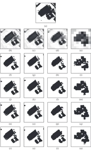
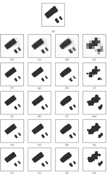
Figure 3 and figure 4 is an image of vegetation and pool. Figure 3(a) is the ground truth image for the vegetation and figure 4(a) is the ground truth image for the pool. While figure 3(b)-3(e) and 4(b)-4(e) is the coarse image for zoom factor 2, 5, 10 and 20. From the output image, for both types of classes, it is shown that the HNN techniques generates better output in zoom factor of 2 than the output in zoom factor of 20. The output image accuracy is affected by the coarse image resolution. As the zoom factor is increased; the output accuracy for each method is decreased. But the output image of each method is almost the same to each other. Therefore it is proven that there are only a slight different of accuracy between the four methods.
vegetation Water bodies Buildings Roads
Table 1 presents the accuracy of each method to classify land covers in different level of image spatial degradation, from a zoom factor of 2 to a zoom factor of 20. Table 2 presents the number of iterations, time taken and accuracy of each method in different zoom factor, from zoom factor of 2 to zoom factor of 20.
Table 1 and Table 2, verifies that the accuracy produced by different ODE methods of HNN only show slight difference. Table 2 shows that Adams-Moulton used the least number of iterations compared to the other three ODE methods. From table 2, there are a huge different in number of iterations taken by each method. As shown, Euler method take 1000 iteration to generates almost the same accuracy as the other three methods. And Adams-Moulton uses just a small number of iterations to generate the same output as Euler.
FIGURE 2. Land cover representation for Figure 1(a) and 1(b) with zoom factor of 20 using different ODE methods for HNN. (a)-(d) Ground truth image. (e)-(h) Coarse images (i)-(l) Results of Euler
ODE (m)-(p) Results of improved Euler ODE (q)-(t) Results of Runge-Kutta ODE. (u)-(x) Results of Adams-Moulton ODE.
FIGURE 3. vegetation’s class representation of figure 1(c) with zoom factor of 2, 5, 10, and 20 using different ODE methods for
HNN. (a) Ground truth image. (b)-(e) Coarse spatial resolution images (f)-(i) Results of Euler ODE (j)-(m) Results of improved Euler ODE (n)-(q) Results of Runge-Kutta ODE. (r)-(u) Results of
FIGURE 4. Pool’s class representation of figure 1(c) with zoom factor of 2, 5, 10, and 20 using different ODE methods for HNN. (a) Ground truth image. (b)-(e) Coarse spatial resolution images,
(f)-(i) Results of Euler ODE, (j)-(m) Results of improved Euler ODE, (n)-(q) Results of Runge-Kutta ODE, (r)-(u) Results of
Adams-Moulton ODE.
TABLE 1. Accuracy of Figure 1(a) and 1(b) for ODE methods s for HNN with different zoom factors.
Zoom Land Improved Runge- Adams-
factor covers Euler Euler Kutta Moulton
2 Plants 84.39 89.79 89.79 89.83 Water 97.62 97.09 97.13 97.11 Building 80.06 79.78 79.72 79.77 Roads 86.87 87.11 87.12 87.08 5 Plants 85.49 91.76 91.84 91.77 Water 97.05 96.11 96.12 96.09 Building 77.92 79.55 79.58 79.54 Roads 85.88 86.65 86.67 86.60 8 Plants 85.59 90.70 90.71 90.74 Water 96.24 95.25 95.22 95.31 Building 75.20 78.26 78.28 78.22 Roads 84.78 85.61 85.61 85.55 10 Plants 85.53 90.04 90.08 90.08 Water 95.56 94.54 94.61 94.63 Building 75.35 77.70 77.81 77.81 Roads 83.99 84.55 84.46 84.56 20 Plants 85.16 86.52 86.59 86.68 Water 92.32 91.36 91.49 91.25 Building 71.99 73.95 73.51 73.92 Roads 76.60 76.37 76.20 76.26
Table 2 also certifies that the other three methods which are Improved Euler, Runge-Kutta and Adams-Moulton are faster than Euler method. Most of it have more than 90% faster than Euler. Table 2 also shows that Adams-Moulton have the lowest time taken to classify the class for the land cover mapping using SRM better than the other three methods.
General trend demonstrated that as the image spatial degradation increased, the average accuracy of all the methods decreased as shown in Figure 5. This situation arises because higher zoom factor reduces the image quality severely. Analysis on the speed of the numerical iteration of different ODE methods of HNN is illustrated in Figure 6. The speed of conventional Euler is the slowest, while Adams-Moulton ODE is the fastest. Adams-Moulton ODE took about half than the time for the Euler to map the land covers output.
FIGURE 6. Average speed by different ODE methods FIGURE 5. Average accuracy by different ODE methods and
CONCLUSION
This paper present different ODE methods to solve HNN problems. As the remote sensing data involve huge data, the speed of the iteration of the HNN is important. Here, using advanced ODE methods, especially Adams-Moulton, demonstrated faster land cover mapping representation than that using conventional Euler method while maintain its accuracy that is comparable to the conventional method. Future works will investigate larger area of site and more land cover classes.
ACKNOWLEDGEMENT
Funding by the Ministry of Higher Education Malaysia under the research grant FRGS/2/2013/TK03/UKM/02/5 is gratefully acknowledged.
REFERENCES
Ardila, J. P., Tolpekin, v. A., Bijker, W. & Stein, A., 2011. Markov-random-field-based super-resolution mapping for identification of urban trees in vHR images. Journal of Photogrammetry and Remote Sensing 66(6): 762-775.
Atkinson, P.M., 2005. Sub-pixel target mapping from soft-classified, remotely sensed imagery. Photogrammetric Engineering and Remote Sensing 71(7): 839-846. Beltran, R.F., Carmona, P.L. & F. Pla, 2017. Single-frame
super-resolution in remote sensing: a practical overview.
International Journal of Remote Sensing 38(1): 314-354.
Butcher, J. C. 2008. Numerical Methods for Ordinary Differential Equations. 2nd edition. John Wiley & Sons.
DigitalGlobe. 2014. QuickBird. https://www.satimagingcorp. com/satellite-sensors/quickbird/
Epperson, J. F. 2013. An Introduction to Numerical Methods and Analysis. Second edition. John Wiley & Sons. Gebregiorgis, S. & Gofe, G. 2016. Research article the
comparison of runge-kutta and adams-bashforh-moulton methods for the first order ordinary differential equations. International Journal of Current Research 8(03): 27356-27360.
Li, X., Du, Y., Ling, F., Feng, Q. & Fu, B., 2014. Superresolution mapping of remotely sensed image based on Hopfield neural network with anisotropic spatial dependence model. IEEE Geoscience and Remote Sensing Letters 11(7): 1265-1269.
Ling, F., Du, Y., Xiao, F., Xue, H. & Wu, S., 2010. Super-resolution land-cover mapping using multiple sub-pixel shifted remotely sensed images. International Journal of Remote Sensing 31(19): 5023-5040.
Ling, F., Foody, G. M., Ge, Y., Li, X. & Du, Y. 2016. An Iterative Interpolation Deconvolution Algorithm for Superresolution Land Cover Mapping. IEEE Transactions on Geoscience and Remote Sensing 54(12): 7210-7222.
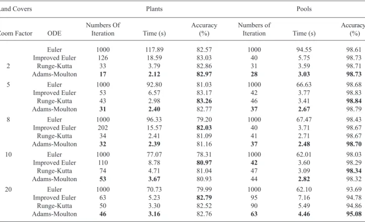
Nguyen, Q. M., Atkinson, P. M., Lewis, H. G. & Al, E, 2011. Super-resolution mapping using Hopfield neural network TABLE 2. Results of Figure 1(c) for ODE methods for HNN with different zoom factors
Land Covers Plants Pools
Numbers Of Accuracy Numbers of Accuracy
Zoom Factor ODE Iteration Time (s) (%) Iteration Time (s) (%)
Euler 1000 117.89 82.57 1000 94.55 98.61 Improved Euler 126 18.59 83.03 40 5.75 98.73 2 Runge-Kutta 33 3.79 82.86 31 3.59 98.71 Adams-Moulton 17 2.12 82.97 28 3.03 98.73 5 Euler 1000 92.80 81.03 1000 66.63 98.68 Improved Euler 53 6.57 83.17 42 3.77 98.83 Runge-Kutta 43 2.98 83.26 46 3.41 98.84 Adams-Moulton 31 2.40 82.77 37 2.67 98.79 8 Euler 1000 96.33 79.20 1000 67.47 98.43 Improved Euler 202 15.57 82.03 40 3.71 98.67 Runge-Kutta 34 2.41 81.09 41 2.71 98.67 Adams-Moulton 32 2.39 81.16 37 2.48 98.70 10 Euler 1000 77.07 78.31 1000 62.01 98.03 Improved Euler 110 8.78 80.97 42 3.60 98.29 Runge-Kutta 74 4.71 81.04 47 3.09 98.34 Adams-Moulton 53 3.67 80.93 44 2.82 98.32 20 Euler 1000 70.73 79.99 1000 62.10 93.69 Improved Euler 63 5.23 82.79 95 7.16 94.78 Runge-Kutta 50 3.30 82.52 90 5.49 94.86 Adams-Moulton 46 3.16 82.76 63 4.46 95.08
with panchromatic imagery. International Journal of Remote Sensing 32(21): 6149-6176.
Press, W. H., Teukolsky, S. A., vetterling, W. T. & Flannery, B. P, 2007. Numerical Recipes: The Art of Scientific Computing. Third edition. New York: Cambridge University Press.
Su, Y., Foody, G. M., Member, S., Muad, A. M. & Cheng, K, 2012. Combining Hopfield neural network and contouring methods to enhance super-resolution mapping. IEEE Journal of Selected Topics in Applied Earth Observations and Remote Sensing 5(5): 1403-1417.
Su, Y., Foody, G. M., Member, S., Muad, A. M. & Cheng, K, 2012. Combining pixel swapping and contouring methods to enhance super-resolution mapping. IEEE Journal of Selected Topics in Applied EarthObservations and Remote Sensing 5(5): 1428-1437.
Tatem, A.J., Lewis, H.G., Atkinson, P.M. & Nixon, M.S., 2001. Super-resolution target identification from remotely sensed image using a Hopfield neural network. IEEE Transactions on Geoscience and Remote Sensing 39(4): 781-796.
Tatem, A.J., Lewis, H.G., Atkinson, P.M. & Nixon, M.S., 2001. Multiple-class land-cover mapping at the sub-pixel scale using a Hopfield neural network.
International Journal of Applied Earth Observation and Geoinformation 3(2): 184-190.
Tatem, A.J., Lewis, H.G., Atkinson, P.M. & Nixon, M.S., 2002. Super-resolution land cover pattern prediction using a Hopfield neural network. Remote Sensing of Environment 79: 1-14.
Wang, Q., Shi, W., Atkinson, P. M., Li, Z. & Member, S. 2015. Land Cover Change Detection at Subpixel Resolution With a Hopfield Neural Network. IEEE Journal of Selected Topics in Applied Earth Observations and Remote Sensing8(3): 1339-1352.
Xu, X., Zhong, Y., Zhang, L. & Member, S, February 2014. Adaptive subpixel mapping based on a multiagent system for remote-sensing imagery. IEEE Transactions on Geoscience and Remote Sensing 52(2): 787-804. Yang, X., Xie, Z., Ling, F., Li, X., Zhang, Y. & Zhong, M,
2018. Spatio-temporal super-resolution land cover mapping based on fuzzy c-means clustering. Journal of Remote Sensing 10: 1212.
Zaki, S. K. M. & Muad, A. M. 2015. Estimating Location of Land Cover Patch in Super-Resolution Mapping By Hopfield Neural Network. 2015 IEEE Symposium on Computer Applications and Industrial Electronics (ISCAIE) Langkawi, 42-47.