Reducing the Impacts of Intra-class Spectral Variability on the Accuracy of
Soft Classification and Super-resolution Mapping of Shoreline
Huong.T.X. Doan 1, Giles M.Foody 2, and Dieu Tien Bui 3,4,*
1 Department of International Cooperation, Ministry of Natural Resources and Environment, Hanoi, Vietnam. E-mail: [email protected]
2 School of Geography, University of Nottingham, Nottingham, NG7 2RD, UK. E-mail: [email protected]
3 Geographic Information Science Research Group, Ton Duc Thang University, Ho Chi Minh City, Vietnam
4 Faculty of Environment and Labour Safety, Ton Duc Thang University, Ho Chi Minh City, Vietnam
* Corresponding author: [email protected] (D. Tien Bui)
ABSTRACT
The main objective of this research is to assess the impact of intra-class spectral variation on the accuracy of soft classification and super-resolution mapping. The accuracy of both analyses was negatively related to the degree of intra-class spectral variation, but the effect could be reduced through use of spectral sub-classes. The latter is illustrated in mapping the shoreline at a sub-pixel scale from Landsat ETM+ data. Reducing the degree of intra-class spectral variation increased the accuracy of soft classification, with the correlation between predicted and actual class coverage rising from 0.87 to 0.94, and super-resolution mapping, with the RMSE in shoreline location decreasing from 41.13 m to 35.22 m.
Keywords: Intra-class spectral variability; Soft classification; Super-resolution mapping; Hopfield Neural Network; Contouring Based method; Shoreline mapping
1.
Introduction
Land cover mapping through the means of an image classification is one of the most common applications of remote sensing. However, the full potential of remote sensing as a source of land cover information is often unrealized due mainly to a set of technical problems. One of the most important problems limiting classification accuracy is that of mixed pixels (Fisher 1997; Cracknell 1998; Foody 2002b; Costa, Foody, and Boyd 2017), which are often abundant in remotely sensed imagery and cannot be appropriately or accurately classified by conventional (hard) image classifiers that associate each pixel to a single land cover class. Soft or fuzzy classification techniques allow for the partial and multiple class membership within each mixed pixel, and, therefore, may be used to refine the standard mapping process as well as increase the accuracy of land cover mapping from remote sensing (Wang 1990; Foody and Cox 1994; Doan and Foody 2007; Mather and Tso 2016).
The output of a soft classification is typically a set of fraction images that show the predicted coverage of each thematic class in the area represented by each pixel. This fractional value is often expressed as a proportion of the area of the pixel covered by the relevant class. Soft classifications have been found to provide more informative and potentially more accurate representations of land cover than conventional hard classifications (Foody 1996; Khatami, Mountrakis, and Stehman 2017). Although soft classifications predict the proportion of each land cover class within each pixel they do not indicate where the land cover classes are spatially located within the pixels. The sub-pixel class components may, however, be located geographically through super-resolution mapping analysis (Tatem et al. 2001; Atkinson 1997).
SRM may be considered as a downscaling technique that predicts the location of land cover classes within each image pixel from the fraction images derived from soft classification. Basically, SRM in remote sensing, a pixel is delineated in a matrix of sub-pixels where each sub-pixel will be predicted to a land-cover class based on the spatial dependence concept. A variety of methods have been used for super-resolution mapping in remote sensing, including those based on spatial
Markov random fields (MRF) (Kasetkasem, Arora, and Varshney 2005), attraction models (Mertens et al. 2006; Wang and Wang 2017), indicator geostatistics (Boucher and Kyriakidis 2006), interpolation method (Ling et al. 2013; Wang, Shi, and Atkinson 2014), adaptive mapping methods (Zhong et al. 2015; Xu, Zhong, and Zhang 2014), and spatial distribution mapping strategy (Ge et al. 2016). Moreover, combinations of methods may be used such as PSM, HNN and MRF (Li, Ling, et al. 2016), BpNN and GA (Li et al. 2015) and contouring and PSM (Su et al. 2012b). In addition, methods may be refined to accommodate for sensor variables such as the point spread function (Wang and Atkinson 2017) and availability of ancillary data sets such as maps or fine spatial resolution imagery (Li et al. 2017). Central to each is the aim to locate the sub-pixel class composition provided by some form or pixel unmixing or soft classification analysis.
To reduce the impact of soft classification error, some algorithms have been proposed to release the constraints of class area fractions i.e. regularization model (Ling et al. 2014) and local endmember method (Li, Zhang, et al. 2016). Some approaches seek to maintain the class proportion information predicted by the unmixing (Foody, Muslim, and Atkinson 2005; Foody and Doan 2007). This may be unwise as it effectively assumes that each class can be represented by a single spectral end-member. Since land cover classes generally display some degree of intra-class spectral variation this assumption is untenable. Moreover, as a result of the intra-class spectral variation it must be noted that the spectral response noted for an image pixel could be associated with a range of land cover compositions, not just a single composition associated with the use of a single end-member per-class.
Indeed, the accuracy of unmixing or soft classification analyses may be negatively related to the degree of intra-class variation present (Foody and Doan 2007; Jay et al. 2017; Huang et al. 2016) and approaches to refine basic unmixing methods to accommodate for this issue have been developed (Song 2005; Xie et al. 2016). Rather than use a single end-member per-class to derive a single class composition estimate in an unmixing analysis a bundle of end members may be used (Bateson, Asner, and Wessman 2000) or a distribution of possible fractional covers could be obtained (Foody and Doan 2007). This distribution may provide a richer description of the possible sub-pixel class compositions of mixed pixels. Although this provides more information, perhaps in the form of a range of possible locations for a class boundary it may be preferable to reduce the impacts of intra-class variability on unmixing and so on super-resolution mapping.
This paper aims to explore and assesss impacts of intra-class spectral variability on the accuracy of unmixing and ultimately super-resolution mapping. Particular attention is focused on the potential to increase the accuracy of the soft classification and super-resolution mapping by reducing the degree of intra-class variation, here through the inclusion of spectral sub-class information into the analysis. Attention is focused on a simple scenario, the fitting of an instantaneous shoreline to imagery unmixed into land and water classes.
2.
Backgound of the methods used
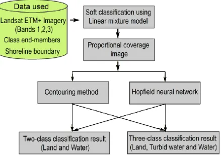
Because the input to a super-resolution mapping analysis is fraction imagery describing the class composition of the image pixels; therefore, many techniques may be used to derive the latter information (Settle and Drake 1993; Song 2005). The resulting fraction images provide the class composition information which may then be located in space via a super-resolution analysis. In this research, Linear mixture model, which is an efficient method for estimating fractional compositions from multispectral images (Settle 2006), was used. From the range of super-resolution mapping methods available, two methods were selected for this study, Contouring method (Foody, Muslim, and Atkinson 2005) and Hopfield neural network (HNN) (Tatem et al. 2002). The contouring method was selected because it is considered as the easiest method used for predicting the location of a boundary at a sub-pixel scale (Su et al. 2012a) whereas HNN has proven in providing accurate sub-pixel classification (Nguyen, Atkinson, and Lewis 2011; Li, Du, et al. 2014), and recently, HNN has been demonstrated to be a successful tool and considered as the most widely used for super-resolution land cover mapping (Su et al. 2012a; Li, Ling, et al. 2014; Wang et al. 2015).
2.1 Linear mixture model
Linear mixture model (LMM) uses a linear mixture assumption that the derived spectral response at an image pixel is a linear combination of the reflectance of all components within that pixel (Settle and Drake 1993); therefore LMM can be expressed in a mathematical form (Haertel and Shimabukuro 2005) as below:
The fraction fjis subjected to the following constrains: 0 and m1 j 1
j
j f
f
(2)2.2 The contouring method
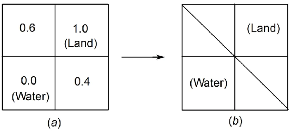
The contouring method is a simple generalization of the soft classification output in which a contour or isoline of class membership is fitted to the fraction imagery to represent the shoreline (Figure 1). The contouring approach to super-resolution mapping involves fitting of a 0.5 class membership contour to the soft classification that indicates the proportional cover of the two classes to be represented. In other words, regardless of fraction value of pixel, the 0.5 class membership is always assigned equally for each of the two classes.
The contour fitted to the output of a soft classification provides a representation of the boundary of land cover patches. Here, a 0.5 class membership contour was used to separate two classes: a target object and its background. This approach allows the contour to run through pixels and can provide smooth boundaries rather than unrealistic jagged ones that arise when boundaries are fitted to hard classifications and constrained to lie between pixels.
Figure 1. Contouring process: (a) a proportion image of soft classification: 0.6 and 0.4 are values which indicate the proportions that are predicted to be land; (b) a contouring line derived from soft classification output.
This method has been applied previously to mapping the shoreline from remotely sensed data (Foody 2002a; Foody, Muslim, and Atkinson 2005) and is simple and quick to undertake. However, one potential drawback of the contour method to shoreline mapping is that the class proportional information provided by the soft classification is not maintained in fitting the contour. Thus, the generalization process involved in fitting the contour can lead to a different class composition
within the area represented by a pixel than that predicted from the unmixing analysis, which could be problematic if the unmixing analysis was highly accurate.
2.3 Hopfield neural network
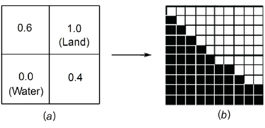
The HNN based approach is computationally more demanding than the contour-based approach; however, this method has been demonstrated to be a successful tool for super-resolution land cover mapping based on the output of soft classification (Nguyen, Atkinson, and Lewis 2011; Su et al. 2012a; Li, Ling, et al. 2014; Wang et al. 2015). With the HNN-based approach the area represented by each pixel is sub-divided into a large number of sub-pixels. Each sub-pixel is given a hard class label with the proportion of a pixel’s sub-pixel components allocated to a class reflecting that predicted for the pixel by the unmixing analysis. The sub-pixels are then spatially re-arranged within the area represented by a pixel until a suitable geographical representation has been derived. A fuller detail on this method can be found in Tatem et al. (2002) but some of the salient features are outlined below.
The HNN is used as an optimization tool, in which, it is initialized randomly using the class composition estimates from a soft classification and run until it converges to a monotonic stable state (Tatem et al. 2002). The zoom factor, z, determines the increase in spatial resolution from the original remotely sensed imagery, which was used to derive soft classification output, to the new fine spatial resolution image. After convergence to a stable state, the output values of all neurons of the network were either 0 or 1, representing a binary classification of the land cover at the finer spatial resolution. The specific goals and constraints of the HNN energy function determined the final distribution of neuron output values. The energy function can be defined as,
( G11 i j, 2G2i j, 3 i j, 4 i j, ) i j
E
k k k P k M (3)where k1, k2, k3and k4 are weighting coefficients which define the effects of the corresponding two goal functions (G1i,j and G2i,j), proportion constraint (Pi,j) and multi-class constraint (Mi,j) to the
Figure 2. HNN process: (a) a proportion image of soft classification: 0.6 and 0.4 are values which indicate the proportions that are predicted to be land; (b) a binary image derived from soft classification output.
Using the class proportion images derived from soft classification (i.e. LMM) as the input, the HNN is implemented using carefully selected settings for the parameters, k1, k2, k3 and k4, as they control the optimisation process of the network. Typically, identifying the optimum weighting constraint values is a difficult and tedious task, so estimates based on certain assumptions and multiple network trial runs are often used (Tatem et al. 2002). In addition, a zoom factor, z, which determines the increase in spatial resolution from the original remotely sensed imagery to the new fine spatial resolution imagery, should also be specified. Finally, the analyst must also define the number of iterations for the analysis.
The output of the HNN approach is a set of binary images with a spatial resolution that is z
times finer than that of the input class proportional images derived from soft classification (Figure 2). The number of the binary images is equal to the number of land cover classes to be mapped with each image representing the location of a defined class. When, as in this study, only two classes are used the boundary between them may be represented by a vector line fitted between sub-pixels with different labels.
3.
Methodology
Figure 3. Methodological flow used in this research
3.1 Data used
Methodological flow of this study is shown in Figure 3. The focus was on mapping part of the shoreline of the Isle of Wight, UK, from Landsat ETM+ data (Figure 4a). It was apparent from Figure 4 that there was a large degree of intra-class spectral variation. The water class, for example, showed clear variation in terms of turbidity. Since the spectral variability, which is central to this research, was most evident in the shorter wavelength data only, the three shortest wavelength bands (ETM+ band 1, band 2 and band 3) were used for the analyses.
The original 30 m spatial resolution ETM+ image was classified visually into two classes, land and water, for use as a ground or reference data set. The classified image was then vectorised along the boundary between land and water classes to generate the reference shoreline. The same procedure was used for separating two spectral sub-classes, turbid water and clear water.
Figure 4. (a) Location of the study area in part of Isle of Wight, UK. (b) Three-band composite Landsat ETM+ images using bands 3, 2, and 1 mapped to red, green, and blue. (c) Black and white image which was converted from the three-band composite Landsat ETM+ images. (d)
Spatially degraded image derived from the black and white image.
The Landsat ETM+ image was spatially degraded by a factor of 10 to simulate data sets with a relatively coarse spatial resolution of 300 m (Figure 4b). This coarse spatial resolution is comparable, in terms of pixel size, to that of the system such as MODIS and MERIS (Justice and
Tucker 2009). The spatially degraded image was obtained by aggregating pixels to the desired spatial resolution, with each degraded DN expressed as the mean DN of the original undegraded pixels it comprised; this is not an ideal simulation of coarse spatial resolution data but provides a common, spatially coarse, data set for the research similar to that used in other studies. The simulated coarse spatial resolution image produced by the degradation process was used in the analyses to predict the shoreline location using super-resolution mapping methods based on the outputs of a soft classification. Since the shoreline mapping is based on a soft classification, the accuracy of the soft classification is critical as it will impact on the ability to derive an accurate representation of the shoreline. The testing set used to assess the accuracy of the soft classifications contained 5000 pixels drawn randomly from the degraded data.
3.2 The impacts of intra-class spectral variation on the use of soft classification for
super-resolution mapping
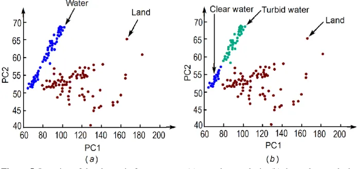
Using the simulated coarse spatial resolution image, a soft classification of the image into the land and water classes was derived through the use of the linear mixture model (Settle and Drake 1993). This analysis was called the two-class analysis. The class end-members required for the linear mixture model were derived from a sample of 180 randomly selected pure pixels, comprising 90 pixels of each class. For illustrative purposes, the data set was also subjected to a principal components analysis, and the first two components were used to display the classes in feature space (Figure 5a). The accuracy of the soft classification was evaluated using correlation coefficient (r) and root mean square error (RMSE) between the predicted and reference coverage.
Figure 5. Location of the classes in feature space: (a) two-class analysis; (b) three-class analysis. The output of the soft classification was an estimate of the proportional coverage of the two classes in each pixel. The contouring and HNN approaches were then used to derive super-resolution maps depicting the shoreline from the soft classification. The zoom factor, z, of the HNN was set to 10, to illustrate the potential to zoom from 300 to 30 m. As in previous studies i.e. Tatem et al. (2001); (2002), the weighting coefficients in equation 3 in this research were be set equal values. The magnitude of the weighting coefficients was, however, varied and six different scenarios set over the range from 70 to 200 were evaluated. The accuracy of the shoreline predictions derived from both the contouring and HNN based approaches to super-resolution mapping was compared against the shoreline represented in a hard classification of the original, spatially undegraded, Landsat ETM+ imagery.
Initially, the shoreline boundary was derived using the single prediction from the conventional linear mixture model in which the centroid of each class was taken to represent its end-member response. The class centroids derived from the training data, however, do not fully describe the characteristics of the classes spectrally; the centroid represents just one point in the data cloud for a class in feature space. The use of a single pixel provides only one possible description of the endmember and does not recognize the potentially large amount of endmember variability and associated impacts (Somers et al. 2011). Since a single class endmember and single composition estimate for each pixel may be unrealistic a distribution of possible class composition estimates for each pixel was derived (Foody and Doan 2007). This was based on running the linear
mixture model repeatedly, using the spectral response of every training pixel as the end-member of the relevant class. The distributional information could be used to indicate the variety of possible class compositions with, for example, the range between the 5th and 95th percentiles of the distribution used to summarise key characteristics.
The accuracy of the shoreline mapping was evaluated using the average distance and RMSE between the predicted and reference shoreline locations. The perpendicular distance between the predicted and actual location of the shoreline was measured at each point every 10 m along the selected stretch of shoreline (Figure 4) and its RMSE was calculated. The length of the shoreline in this study area was about 41.68 km. The range of possible shoreline positions was indicated by the average distance between the shorelines represented by the 5th and 95th percentiles of the class composition generated.
To reduce the impacts of intra-class spectral variation on the soft classification and super-resolution mapping, the water class was divided into two spectral sub-classes, turbid water and clear water. In this case, the unmixing analysis essentially focused on three classes, yielding fraction images depicting the proportion cover of land, turbid water and clear water. For comparability with the earlier work, the training set for each class comprised 90 pixels (Figure 5a). This analysis is hereafter described as the three-class analysis. Comparison of the accuracy of the soft classification derived in this way and of the shorelines fitted to those associated with the earlier analysis would indicate the potential value of reducing the intra-class spectral variation on super-resolution mapping.
4.
Results and Discussion
Sub-pixel class composition estimates for the two original classes, land and water, were derived for each pixel in the spatially degraded imagery. Initially, the end-members were defined as the class centroids for input to the conventional LMM. There was a strong relationship between predicted and actual fractional cover (r = 0.87; RMSE = 0.26) (Table 1). This suggests that the soft classification outputs were accurate and could be used to derive shoreline map.
Two-class analysis Water 0.87 0.27
Average 0.87 0.27
Land 0.94 0.20
Three-class analysis Turbid water 0.96 0.20
Clear water 0.92 0.21
Average 0.94 0.20
The shorelines were derived using two approaches, the contouring and HNN, based on the output of the sub-pixel class compositions. Using the class proportion images derived from a soft classification as the input, the HNN is implemented using a selected set of parameters (Equation 3) which should be carefully chosen by the user. They are four weighting constants: k1,k2,k3 and k4
, a zoom factor z and the number of iterations for the performance of the network. The values of the goal and weighting constraints estimation were derived via certain assumptions and multiple network trial runs. Tatem et al. (2001, 2002) suggest that the weighting constants should be equal for obtaining the highest performance and found, for their study, that an optimal value was 150. In this research, several trial networks were run with different values of the weighting constants (Table 2), the zoom factor of 10, and number of iterations of 5000. The highest accuracy of shoreline mapping was obtained with the weighting constants of k1 k2 k3 k4 70 and all the HNN-based results presented in this paper are HNN-based on analyses that used these settings.
Table 2. Accuracy of shoreline mapping derived from trial HNN (k1,k2,k3,k4are the two goal functions, proportion, and multi- class weighting constants, respectively).
Weighting constants Accuracy of shoreline mapping
1
k k2 k3 k4 Average distance (m) RMSE (m)
70 70 70 70 45.00 41.13
100 100 100 100 53.10 44.92
150 150 150 150 47.50 43.37
170 170 170 170 47.06 42.90
200 200 200 200 47.31 43.12
The output of the HNN approach is a set of binary images with a spatial resolution that is z times finer than that of the input class proportional images derived from soft classification. In the analyses of this research the HNN was undertaken with a zoom factor of 10. With that zoom factor applied for the input proportion images with spatial resolution of 300 m, the HNN was produced the output maps with a spatial resolution of 30m which was equal to the spatial resolution of reference image. The number of the binary images is equal to the number of land cover classes to be mapped with each image is shown the location of a defined class. In this study, with the purpose of shoreline mapping, the remotely sensed imagery used was mapped to two land cover classes water and land. The binary images derived from the HNN approach were then vectorised along the boundary between the land and water classes to generate the shoreline.
Figure 6a shows the shoreline in a part of study area derived from the HNN approach as an example and Table 3 illustrates the accuracy of the predicted shorelines derived.
Method Contouring HNN Average distance (m) RMSE (m) Average distance (m) RMSE (m) Two-class analysis 41.91 38.57 45.00 41.13 Three-class analysis 32.76 28.12 37.70 35.22
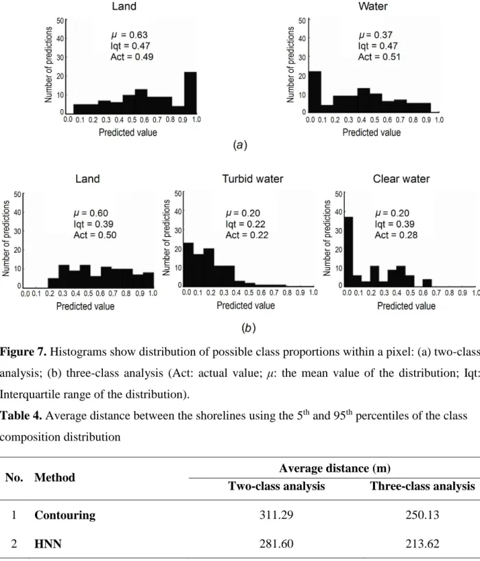
For each image pixel, a distribution of possible class proportion was derived by mixing the distributions of the pure land and water pixels used to train the mixture model (Figure 7). The distributions derived for the area represented by a pixel in each image may then use to derive an alternative indication of shoreline and it may be preferable to be aware of the range of possible shoreline positions. For illustrative purposes, the locations of the shorelines using the 5th and 95th percentiles of the class composition distributions were generated. The nature of the distribution of possible mixing predictions for an image pixel will depends on the location of the point in feature space and the degree of intra-class variation and class co-variation present. This may impact on the width of the zone of possible shoreline locations, bounded by the 5th and 95th percentiles of land coverage.
Figure 7. Histograms show distribution of possible class proportions within a pixel: (a) two-class analysis; (b) three-class analysis (Act: actual value; μ: the mean value of the distribution; Iqt: Interquartile range of the distribution).
Table 4. Average distance between the shorelines using the 5th and 95th percentiles of the class composition distribution
No. Method Average distance (m)
Two-class analysis Three-class analysis
1 Contouring 311.29 250.13
the single set of class proportion predictions as input for super-resolution mapping may be unwise and the distribution of possible predictions may be used to provide a richer interpretation for this process. Furthermore, if the uncertainty of the distribution is large, there may be a problem for the applications of using soft classification such as change detection and super-resolution mapping (Foody and Doan, 2007).
Figure 8. The zone of possible shoreline locations in the area highlighted in Figure 4a, bounded by the 5th and 95th percentiles using HNN approach (a) two-class analysis; (b) three-class analysis. The potential to reduce the impacts of intra-class spectral variation on the accuracy of soft classification and super-resolution mapping by a defining spectral sub-class was illustrated by the three-class analysis. It was apparent that the accuracy of the predictions from three-class analysis (r = 0.94, significant at 0.01 significance level) was much higher than that from two-class analysis (r = 0.87, significant at the 0.01 significance level).
Figure 8 shows the shoreline positions derived from the output of soft classification of both the two-class and three-class analyses using HNN based approach as an example. For the purpose of the comparison, Table 3 shows the accuracy of the shoreline mapping from these two analyses and highlights that with both approaches used to generate shorelines the accuracy of the shoreline mapping in three-class analysis was higher than that in two-class analysis. For example, using HNN based approach to derive shoreline mapping, three-class analysis provided the shoreline with higher accuracy (RMSE = 35.22 m) than two-class analysis (RMSE = 41.13 m). It was suggested that the reduction of the intra-class spectral variability increased the accuracy of soft classification and shoreline mapping.
In terms of the distribution of class composition estimates for each pixel, according to Table 4, the average ranges of possible shoreline positions derived from both the contouring and HNN
based approaches in three-class analysis was smaller than that from two-class analysis. For example, using HNN based approach the width of the zone of possible shoreline locations, bounded by the 5th and 95th percentiles of land coverage, was narrower, 213.62 m, from the three-class analysis (Figure 6b) than that from two-class analysis (Figure 6a), 281.60 m. Similar trends were noted for the results based on the contouring approach (Table 4).
5.
Conluding remarks
Mixed pixels are one of the main problems limiting the accuracy of mapping land cover from remotely sensed imagery. Soft classifications allow for partial and multiple class membership of mixed pixels and can give a more accurate and realistic representation of land cover than a hard classification. A further refinement may be made by locating geographically the sub-pixel class composition estimates depicted in a soft classification through super-resolution mapping. Some super-resolution mapping approaches attempt to maintain the class proportion information output from a soft classification as based on the assumption that a class can be represented by a single spectral end-member. This may be unrealistic as classes typically display a degree of spectral variability and the accuracy of soft classification is negatively related to the degree of intra-class variation present.
The impacts of intra-class spectral variation on the accuracy of soft classification and super-resolution mapping were investigated through analyses with two land cover classes ( land and water) and then three classes (with the water class sub-divided into turbid and clear water). The three-class approach led to the reduction of the intra-class variation of water class compared with two-class analysis and ultimately to an increase in the accuracy of the super-resolution mapping. In terms of the sub-pixel class composition estimates derived by a soft classification, the accuracy of the predictions from three-class analysis (e.g., r = 0.94 and RMSE = 0.20) was higher than that from two-class analysis (e.g., r = 0.87 and RMSE = 0.27). In terms of shoreline mapping, with both approaches used to generate shorelines, the accuracy of the shoreline in three-class analysis was higher than that in two-class analysis. For example, using HNN based approach to derive shoreline
three-class analysis than from two-class analysis. For example, using the contouring approach to derived shorelines, the average distance between the possible shorelines in three-class analysis was 250.13 m, while this number in two-class analysis reached to 311.29 m.
In conclusion, intra-class spectral variation has negative impacts on the accuracy of soft classification and super-resolution mapping derived from the output of soft classification. Reducing the intra-class class spectral variability was a possible approach to decrease the negative impacts of intra-class spectral variability on soft classification and super-resolution mapping. Specifically, reducing the degree of intra-class variation increased the accuracy of soft classification and shoreline mapping accuracy and reduce the range of possible shoreline positions.
Acknowledgement
The authors wish to thank the Global Land Cover Facility (GLCF) sponsored by the University of Maryland for producing Landsat ETM+ data in their present form and distributing them. This paper is an extension of an article presented at the IGARSS conference in Barcelona and submitted with permission of the conference organisers.
Reference
Atkinson, Peter M. 1997. "Mapping sub-pixel boundaries from remotely sensed images." Innovations in
GIS 4:166-80.
———. 2005. "Sub-pixel target mapping from soft-classified, remotely sensed imagery."
Photogrammetric Engineering & Remote Sensing 71 (7):839-46.
Bateson, C Ann, Gregory P Asner, and Carol A Wessman. 2000. "Endmember bundles: A new approach
to incorporating endmember variability into spectral mixture analysis." IEEE Transactions on
Geoscience and Remote Sensing 38 (2):1083-94.
Boucher, Alexandre, and Phaedon C Kyriakidis. 2006. "Super-resolution land cover mapping with indicator geostatistics." Remote Sensing of Environment 104 (3):264-82.
Costa, Hugo, Giles M. Foody, and Doreen S. Boyd. 2017. "Using mixed objects in the training of
object-based image classifications." Remote Sensing of Environment 190:188-97. doi:
https://doi.org/10.1016/j.rse.2016.12.017.
Cracknell, AP. 1998. "Review article Synergy in remote sensing-what's in a pixel?" International Journal of Remote Sensing 19 (11):2025-47.
Doan, Huong TX, and Giles M Foody. 2007. "Increasing soft classification accuracy through the use of an
ensemble of classifiers." International Journal of Remote Sensing 28 (20):4609-23.
Fisher, P. 1997. "The pixel: a snare and a delusion." International Journal of Remote Sensing 18 (3):679-85.
Foody, Giles M. 1996. "Approaches for the production and evaluation of fuzzy land cover classifications
from remotely-sensed data." International Journal of Remote Sensing 17 (7):1317-40.
———. 2002a. "The role of soft classification techniques in the refinement of estimates of ground control
point location." Photogrammetric Engineering and Remote Sensing 68 (9):897-903.
———. 2002b. "Status of land cover classification accuracy assessment." Remote Sensing of Environment
Foody, Giles M, and HTX Doan. 2007. "Variability in soft classification prediction and its implications for sub-pixel scale change detection and super resolution mapping." Photogrammetric Engineering & Remote Sensing 73 (8):923-33.
Foody, Giles M, Aidy M Muslim, and Peter M Atkinson. 2005. "Super‐resolution mapping of the waterline
from remotely sensed data." International Journal of Remote Sensing 26 (24):5381-92.
Foody, GM, and DP Cox. 1994. "Sub-pixel land cover composition estimation using a linear mixture model
and fuzzy membership functions." Remote Sensing 15 (3):619-31.
Ge, Yong, Yuehong Chen, Alfred Stein, Sanping Li, and Jianlong Hu. 2016. "Enhanced subpixel mapping with spatial distribution patterns of geographical objects." IEEE Transactions on Geoscience and Remote Sensing 54 (4):2356-70.
Haertel, Vitor F, and Yosio Edemir Shimabukuro. 2005. "Spectral linear mixing model in low spatial
resolution image data." IEEE Transactions on Geoscience and Remote Sensing 43 (11):2555-62.
Huang, Longhui, Chen Chen, Wei Li, and Qian Du. 2016. "Remote sensing image scene classification using multi-scale completed local binary patterns and fisher vectors." Remote Sensing 8 (6):483.
Jay, Sylvain, Mireille Guillaume, Audrey Minghelli, Yannick Deville, Malik Chami, Bruno Lafrance, and Véronique Serfaty. 2017. "Hyperspectral remote sensing of shallow waters: Considering environmental noise and bottom intra-class variability for modeling and inversion of water
reflectance." Remote Sensing of Environment 200:352-67.
Justice, Christopher Owen, and CJ Tucker. 2009. "Coarse spatial resolution optical sensors." The SAGE
Handbook of Remote Sensing, Sage, London:139-50.
Kasetkasem, Teerasit, Manoj K Arora, and Pramod K Varshney. 2005. "Super-resolution land cover
mapping using a Markov random field based approach." Remote Sensing of Environment 96
(3-4):302-14.
Khatami, Reza, Giorgos Mountrakis, and Stephen V Stehman. 2017. "Predicting individual pixel error in
remote sensing soft classification." Remote Sensing of Environment 199:401-14.
Li, Linyi, Yun Chen, Tingbao Xu, Rui Liu, Kaifang Shi, and Chang Huang. 2015. "Super-resolution mapping of wetland inundation from remote sensing imagery based on integration of back-propagation
neural network and genetic algorithm." Remote Sensing of Environment 164:142-54. doi:
https://doi.org/10.1016/j.rse.2015.04.009.
Li, Wenbo, Xiuhua Zhang, Feng Ling, and Dongbo Zheng. 2016. "Locally adaptive super-resolution
waterline mapping with MODIS imagery." Remote sensing letters 7 (12):1121-30.
Li, Xiaodong, Yun Du, Feng Ling, Qi Feng, and Bitao Fu. 2014. "Superresolution mapping of remotely
sensed image based on hopfield neural network with anisotropic spatial dependence model." IEEE
Geoscience and Remote Sensing Letters 11 (7):1265-9.
Li, Xiaodong, Feng Ling, Yun Du, Qi Feng, and Yihang Zhang. 2014. "A spatial–temporal Hopfield neural network approach for super-resolution land cover mapping with multi-temporal different resolution
remotely sensed images." ISPRS Journal of Photogrammetry and Remote Sensing 93:76-87.
Li, Xiaodong, Feng Ling, Giles M Foody, and Yun Du. 2016. "Improving super-resolution mapping through
combining multiple super-resolution land-cover maps." International Journal of Remote Sensing 37
(10):2415-32.
Li, Xiaodong, Feng Ling, Giles M Foody, Yong Ge, Yihang Zhang, and Yun Du. 2017. "Generating a series of fine spatial and temporal resolution land cover maps by fusing coarse spatial resolution remotely
196:293-Mertens, Koen C, Bernard De Baets, Lieven PC Verbeke, and Robert R De Wulf. 2006. "A sub‐pixel mapping algorithm based on sub‐pixel/pixel spatial attraction models." International Journal of Remote Sensing 27 (15):3293-310.
Mertens, Koen C, Lieven PC Verbeke, Toon Westra, and Robert R De Wulf. 2004. "Sub-pixel mapping
and sub-pixel sharpening using neural network predicted wavelet coefficients." Remote Sensing of
Environment 91 (2):225-36.
Nguyen, Quang Minh, Peter M Atkinson, and Hugh G Lewis. 2011. "Super-resolution mapping using
Hopfield neural network with panchromatic imagery." International Journal of Remote Sensing 32
(21):6149-76.
Settle, Jeff. 2006. "On the effect of variable endmember spectra in the linear mixture model." IEEE Transactions on Geoscience and Remote Sensing 44 (2):389-96.
Settle, JJ, and NA Drake. 1993. "Linear mixing and the estimation of ground cover proportions."
International Journal of Remote Sensing 14 (6):1159-77.
Somers, Ben, Gregory P Asner, Laurent Tits, and Pol Coppin. 2011. "Endmember variability in spectral
mixture analysis: A review." Remote Sensing of Environment 115 (7):1603-16.
Song, Conghe. 2005. "Spectral mixture analysis for subpixel vegetation fractions in the urban environment:
How to incorporate endmember variability?" Remote Sensing of Environment 95 (2):248-63.
Su, Yuan-Fong, Giles M Foody, Anuar M Muad, and Ke-Sheng Cheng. 2012a. "Combining Hopfield neural
network and contouring methods to enhance super-resolution mapping." IEEE Journal of Selected
Topics in Applied Earth Observations and Remote Sensing 5 (5):1403-17.
———. 2012b. "Combining pixel swapping and contouring methods to enhance super-resolution mapping." IEEE Journal of Selected Topics in Applied Earth Observations and Remote Sensing 5 (5):1428-37.
Tatem, Andrew J, Hugh G Lewis, Peter M Atkinson, and Mark S Nixon. 2001. "Super-resolution target
identification from remotely sensed images using a Hopfield neural network." IEEE Transactions on
Geoscience and Remote Sensing 39 (4):781-96.
———. 2002. "Super-resolution land cover pattern prediction using a Hopfield neural network." Remote
Sensing of Environment 79 (1):1-14.
Verhoeye, Jan, and Robert De Wulf. 2002. "Land cover mapping at sub-pixel scales using linear
optimization techniques." Remote Sensing of Environment 79 (1):96-104.
Wang, Fangju. 1990. "Fuzzy supervised classification of remote sensing images." IEEE transactions on
geoscience and remote sensing 28 (2):194-201.
Wang, Peng, and Liguo Wang. 2017. "Soft-then-hard super-resolution mapping based on a spatial attraction model with multiscale sub-pixel shifted images." International Journal of Remote Sensing 38 (15):4303-26.
Wang, Qunming, and Peter M Atkinson. 2017. "The effect of the point spread function on sub-pixel
mapping." Remote Sensing of Environment 193:127-37.
Wang, Qunming, Wenzhong Shi, and Peter M Atkinson. 2014. "Sub-pixel mapping of remote sensing
images based on radial basis function interpolation." ISPRS Journal of Photogrammetry and Remote
Sensing 92:1-15.
Wang, Qunming, Wenzhong Shi, Peter M Atkinson, and Zhongbin Li. 2015. "Land cover change detection
at subpixel resolution with a Hopfield neural network." IEEE Journal of Selected Topics in Applied
Earth Observations and Remote Sensing 8 (3):1339-52.
Xie, Dengfeng, Jinshui Zhang, Xiufang Zhu, Yaozhong Pan, Hongli Liu, Zhoumiqi Yuan, and Ya Yun. 2016. "An improved STARFM with help of an unmixing-based method to generate high spatial and
temporal resolution remote sensing data in complex heterogeneous regions." Sensors 16 (2):207.
Xu, Xiong, Yanfei Zhong, and Liangpei Zhang. 2014. "Adaptive subpixel mapping based on a multiagent
system for remote-sensing imagery." IEEE Transactions on Geoscience and Remote Sensing 52
Zhong, Yanfei, Yunyun Wu, Xiong Xu, and Liangpei Zhang. 2015. "An adaptive subpixel mapping method based on MAP model and class determination strategy for hyperspectral remote sensing imagery."