Metaheuristic tuning of type-II fuzzy
inference systems for data mining
Conference or Workshop Item
Accepted Version
Ojha, V. ORCID: https://orcid.org/0000-0002-9256-1192,
Abraham, A. and Snasel, V. (2016) Metaheuristic tuning of
type-II fuzzy inference systems for data mining. In: 2016 IEEE
International Conference on Fuzzy Systems (FUZZ-IEEE),
25-29 Jul 2016, Vancouver, Canada, pp. 610-617. doi:
https://doi.org/10.1109/FUZZ-IEEE.2016.7737743 Available at
http://centaur.reading.ac.uk/93557/
It is advisable to refer to the publisher’s version if you intend to cite from the
work. See
Guidance on citing
.
Published version at: http://www.scopus.com/inward/record.url?eid=2-s2.0-85006817813&partnerID=MN8TOARS
To link to this article DOI: http://dx.doi.org/10.1109/FUZZ-IEEE.2016.7737743
All outputs in CentAUR are protected by Intellectual Property Rights law,
including copyright law. Copyright and IPR is retained by the creators or other
copyright holders. Terms and conditions for use of this material are defined in
the
End User Agreement
.
www.reading.ac.uk/centaur
CentAUR
Central Archive at the University of Reading
Reading’s research outputs online
Metaheuristic Tuning of Type-II Fuzzy Inference
Systems for Data Mining
Varun Kumar Ojha
∗, Ajith Abraham
†,V´aclav Sn´aˇsel
∗∗IT4Innovations, V ˇSB Technical University of Ostrava, Ostrava, Czech Republic †Machine Intelligence Research Lab, Auburn, WA, USA
[email protected], [email protected], [email protected]
Abstract—Introduction of the fuzzy-set enabled the modeling of uncertain and noisy information. Type-2 fuzzy set took this further ahead by allowing fuzzy membership function to be fuzzy itself. In this work, we discussed an interval type-2 fuzzy inference system (IT2FIS). The training of the IT2FIS was provided in supervised manner by using metaheuristic algorithms. We comprehensively illustrated the formulation of the IT2FIS into an optimization problem. A precise genotype (a real vector) mapping of IT2FIS and a population-based strategy for optimum rule-base selection is described in this work. Since the IT2FIS learning is computationally difficult and costly, which we described in detail in this work, a comprehensive comparison between the performances of the metaheuristic algorithms were examined. The obtained results suggest that the IT2FIS learning was faster at the initial iterations of the metaheuristic learning, but tend to slow and get stuck in local minima. However, the metaheuristic algorithms, differential evaluation and bacteria foraging optimization offered significantly better results when compared to artificial bee colony, gray wolf optimization, particle swarm optimization and the other fuzzy inference models chosen for comparisons from literature.
I. INTRODUCTION
Fuzzy inference system has a vast range of application domain since it does human-like reasoning by modeling am-biguous, uncertain, incomplete, inaccurate, and noisy infor-mation. Initially, we had only type-1 fuzzy set, introduced by Zadeh [1], to addressed such problems, but the fuzzy set type-2 development has drawn much attention towards handling nosy and imprecise data [2]. A fuzzy inference system (FIS) is composed of a fuzzifier that fuzzify input information, an inference-engine that infer information from a rule-base, and a defuzzifier that returns the crisp information. In simple words, an FIS infer the information from a rule-base. Hence, FIS can be described as a set of rules, where rules are in the form: IF-THEN that is antecedent and consequent form. Takagi-Sugeno model [3] is a widely used FIS model that embraced this IF-THEN form, where the antecedent part consists of membership functions (MFs) and the consequent part consists of real value or a function that infer the information depending on the antecedent part.
Type-2 fuzzy-set and type-1 fuzzy-set differs when it comes to the representation of the antecedent part and the represen-tation of the consequent part of a rule in FIS. Unlike the crisp outputs of the type-1 fuzzy set MFs, the output of type-2 fuzzy set MFs are fuzzy in nature. Such nature of MFs in type-2 fuzzy set is advantageous in processing uncertain information
effectively than that of the 1 fuzzy set [4]. Hence, type-2 fuzzy set is able to overcome certain limitations of the type-1 fuzzy set [4]. However, type-2 fuzzy inference system is computationally expensive because of the large number of parameters in the optimization and the type-reduction mechanism required at the defuzzification part. Interval type-2 FIS (ITtype-2FIS), because of its simplification of type-type-2 MF, reduces the computational cost. The MFs in interval type-2 fuzzy set are bounded by an upper MF and a lower MF and the area between the upper MF and the lower MF is called thefootprint of uncertainty[2]. The MFs for FIS are designed by using optimization and the design of MFs for an IT2FIS means the optimization of its parameters. Hence, it is called the optimization of FIS. Therefore, the optimization of the FIS parameters is crucial and the metaheuristics are best suited in this role. Such form of optimization in known as parameter learning or training. In this work, an FIS system was designed by selection of an optimal subset of rules from a population of rules. Such selection was met by using a genetic representation of FIS. Hence, from a population of rules, an optimal subset of rules was selected [5]. Each rule was designed by using type-2 Gaussian MFs, whose parameters were subjected to optimization together with the parameters of the consequent parts of the each rule. Therefore, for a given dataset, FIS posed supervised learning task. The significance of FIS optimization is supported by several successfully application in engineering problems [6], [7].
The metaheuristics are nature-inspired (bio-inspired) algo-rithms that optimize a real vector by searching a vast real-valued search-space. The optimization is met by minimiz-ing/maximizing an objective function. In this, work, the pa-rameters of IT2FIS were formulated into a real vector that was optimized by using different metaheuristic algorithms: artifi-cial bee colony [8], bacteria foraging optimization [9], differ-ential evolution [10], gray wolf optimization [11], and particle swarm optimization [12]. Additionally, different benchmark datasets taken from UCI machine learning repository [A] were used for the experiments. In this work, a comprehensive comparative study between the metaheuristic algorithms was presented. We observed that FIS training was faster at initial stage of metaheuristic training, but tend to slow at the later stages of learning. Additionally, comparative study between metaheuristics from FIS suggest that there differential evolu-tion and bacteria foraging performed in two distinct data set
and none of one algorithm excel in all the case, which is what, no free lunch theoremdescribed by Wolpert and Macready [13] says. Moreover, the performance of the optimized FIS was compared with FIS methods chosen from literature [14], [15], [16], [17], [18].
In the past, researcher used various metaheuristic for FIS optimization [19], [20]. A list of several bio-inspired meta-heuristic algorithms used for the optimization of FIS is offered in [21]. The list consist of detail study of particle swarm optimization, genetic algorithm, and ant colony optimization. Additionally, they offer a comparative study of these bio-inspired algorithm over a mobile robot [22]. Since type-2 FIS is inspired by type-1 FIS, it inherits the idea of modeling for its parameter optimization from type-1 FIS [23]. A detail description of modeling of FIS is provided in [24]. In this work, our focus was on the following dimensions of FIS optimization:
1) Introduction of interval type-2 FIS (Section II-A). 2) Introduction of the metaheuristics (Section II-B). 3) Formulation of interval type-2 FIS as metaheuristic
optimization (Section III).
4) Evaluation of the FIS and metaheuristics (Section IV). 5) Analysis of no free lunch theoremeffect (Section IV). The primary goal of this work was to illustrate usefulness of different metaheuristic in the optimization of IT2FIS for data mining tasks. Specifically, IT2FIS was applied to model regression problems and the performance of IT2FIS was compared to other models available in literature. Additionally, strength of individual metaheuristics were compared.
II. PRELIMINARIES
This section describes the interval type-2 fuzzy inference system (IT2FLS) and the metaheuristic algorithms which are used for optimizing IT2FLS.
A. Interval Type-2 Fuzzy Inference System
A type-2 fuzzy set A˜ is characterized by a 3-dimensional membership function [25]. The three axes of type-2 fuzzy set are defined as follows. The x-axis is called primary variable, the y-axis is called secondary variable (or primary MF, which is denoted by u), and the z-axis is called the MF value (or secondary MF value, which is denoted by µ). Hence, in a universal set X, a type-2 fuzzy set A˜has the form:
˜
A={((x, u), µA˜(x, u))|∀x∈X,∀u∈[0,1]}. (1)
Hence, µ has a 2-dimensional support called the foot print of uncertainty of A˜, which is bounded an upper MF µ¯A˜(x)
and a lower MF µ˜
A(x). The foot print of uncertainty is the
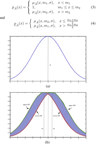
area enclosed within the upper MF and the lower MF (see Fig. 1(b)). A Gaussian function with uncertain mean within
[m1, m2] and standard deviation σ is a interval type-2 MF
(see Fig. 1, which is expressed as:
µA˜(x, m, σ) = exp −1 2 x−m σ , m∈[m1, m2]. (2)
In this work, the upper MF and the lower MF were defined as [2]: ¯ µA˜(x) = µA˜(x, m1, σ), x < m1 1, m1≤x≤m2 µA˜(x, m2, σ), x > m2 (3) and µ˜ A(x) = µA˜(x, m2, σ), x≤ m1+2m2 µA˜(x, m1, σ), x > m1+2m2 (4) 0 1 2 3 4 5 6 7 8 9 10 0 0.1 0.2 0.3 0.4 0.5 0.6 0.7 0.8 0.9 1 m (a) 0 1 2 3 4 5 6 7 8 9 10 0 0.1 0.2 0.3 0.4 0.5 0.6 0.7 0.8 0.9 1 m1 m2 upper MF lower MF lower MF upper MF (b)
Fig. 1. Type-1 MF (a) with meanm= 5.0. Type-2 Fuzzy MF (b) with fixed σ= 2.0and meansm1= 4.5andm2= 5.5. Upper MF in green and lower
MF in red are defined as per (3) and (4).
A FIS with one or more interval type-2 MF is an interval type-2 FIS. The basic blocks of a type-2 FIS is shown in Fig 2. FIS depends on the rule-base, which is in IF-THEN form. Hence, a general form ofMrules for an input vectorx=
{x1, x2, . . . , xn}and corresponding outputyhas the following
form:
Ri:IFx1isA˜i1and . . .andxnisA˜inTHENy isB
i n (5)
Fuzzifier Rule-base Defuzzifier
Type-reducer Inference Engine Crisp Input Crisp Output
where B = [¯b, b] is weights at consequent part of the rule
and i = 1,2, . . . , M. The firing strength of interval type-2
Fi= [ ¯f i, fi]is computed as: ¯ fi= n Y j ¯ µA˜i j and fi= n Y j µ˜ Ai j (6) At this stage, inference engine fires the rule and the type-reducer reduces the type-2 fuzzy set to type-1 fuzzy set. Here, in this work, center of set type-reducer, prescribed by Karnik [2], was used. The center of set ycos is computed as:
ycos= [ fi∈Fn PM i=1f ibi fi = [yl, yr], (7)
where yl and yr are left and right end of interval. For the
acceding order of¯bi andbi
,yl andyr are computed as:
yl= PL i=1f¯ i¯bi+PM i=L+1f ibi PL i=1f¯i+ PM i=L+1f i , (8) yr= PR i=1f i bi+PM i=R+1f¯ i¯bi PR i=1f i +PM i=R+1f¯i , (9)
whereL andR are the switch point, determined by
bL≤yl≤bL+1 and¯bR≤yr≤¯bR+1,
respectively. The defizzified crisp output was computed as:
ˆ
y(x) =yl+yr
2 . (10)
We resorted to using IT2FIS for supervised learning. Hence, for a dataset having N input-output pair{x, y}, the fitness of model created from IT2FIS was computed using root of mean squared error (RMSE). The RMSEE is expressed as:
E= v u u t1 N N X i=1 (yi−yˆi) 2 , (11)
whereyˆandy are the predicted and desired outputs. B. Meta-heuristic Algorithms
Metaheuristic algorithms are nature inspired algorithms that optimize real vector by searching vast search space. To searches through the search-space, metaheuristic algorithms efficiently combines two techniques: exploitation and explo-ration. By exploitation, it creates new solution from the already discovered solutions and by exploration, it searches through new areas of a search space or in other words, it avoids already visited areas of a given search space. There are several types of metaheuristic algorithms. Each metaheuristic algorithm is inspired by a form of natural heuristics. For example, artificial bee colony (ABC), bacteria foraging optimization (BFO), gray wolf optimization (GWO), and particle swarm optimization (PSO) are inspired from the foraging behavior of swarm or animals. On the other hand, differential evolution (DE) and genetic algorithm (GA) are inspired by evolutionary process of natural selection. However, the metaheuristic algorithms
follows a common procedure as laid down in Algorithm 1, but they differ in their respective design of metaheuristic operators, i.e., the heuristics.
Algorithm 1 Meta-heuristic Framework for Optimization 1: procedure META-HEURISTICS-NN(W, )
2: Initialize W0
3: Fittest solutionw∗=f ittest(W0)
4: repeat 5: Wt+1:=MHOperator(Wt) 6: wˆ =f ittest(Wt+1) 7: if w<w∗ then 8: w∗=w 9: end if
10: until Stopping criteria satisfied 11: return w∗
12: end procedure
1) Artificial bee colony (ABC): Karaboga [8] proposed ABC, which is inspired by foraging behavior of honey bee swarm. To find an optimal solution for a given problem ,the ABC algorithm uses a population of bees (solutions) and explore the given search-space. The ABC algorithm works as follows. First, a memory W of initial food positions (solution)
wi={w1, w2, . . . , wD} ∀i= 1,2, . . . , P is initialized, where
P is size of population. Second, the food position wi is
updated by the artificial bees in iterative fashion. Thus, in ABC, thej-th variable of i-th solution is computed as:
wij =wij+rand(−1,1)×(wij−wkj) (12)
where, k ∈ [1, P], j ∈ [i, D], and xij is the comparison
between thei-th food source and a randomly chosen neighbor
k. If no good solution is found for some number of trialstabc
by using (12), then, new solution is computed as:
wij =wmin,j+rand(0,1)(wmax,j−wmin,j), (13)
whereminandmaxis the bound of thej-th variable. Simi-larly, other metaheuristics have their nature inspired heuristics procedure for real vector computation.
2) Bacteria Foraging Optimization (BFO): The heuristic of BFO imitates the social and foraging behavior of bacteria [9]. It mathematical defines the tumbling and the swimming be-havior of bacteria to represent exploration in a search space. Additionally, BFO imitates a bacteria reproduction and death to improve the algorithm’s performance. Hence, the parameters used in BFO are: number reproduction step Nr, number of
death steps Nd, number of tumbling and swim steps Ns,
and, death ratedr. BFO is a complex and efficient algorithm,
provided a careful setting of these parameters.
3) Differential Evolution (DE): DE proposed by Storn and Price [10] is a metaheuristic that uses crossover operator inspired by the mechanisms of “natural selection.” The basic principle of DE is as follows. First, an initial population ofD -dimensional solutions wi are initialized. The creation of new
distinct solutionsa, b, andcand the best solutiongare chosen from P many solutions. Then, a random indexk ∈[1, P] is chosen. Hence, a new solution w0i is constructed as:
w0i=
ai+F(gi−ai) +F(bi−ci) ifri<CR ori=P
xi ifri≥CR ori6=P
(14) where CR indicates the crossover rate, F indicates the weight factor andri is a uniform random sample chosen in (0,1).
4) Genetic Algorithm (GA): GA is inspired by the dynam-ics of evolutionary strategies, i.e., the principles of “the natural selection.” It explores a real-valued search-space by using the genetic operators such as: selection, crossover, and mutation. Theses operators are applied over a current population to generate a new population, iteratively [5]. To generate a new population, a selection operator selects some individuals (solution vectors) from a current population for crossover and mutation operators to create the new individuals for the new population. The selection procedure (e.g., tournament selec-tion), the crossover frequency pcand the mutation frequency
pmgoverns the performance of GA. Letw1∈Wandw2∈W
are two individual solutions. Then a new solution is created by using crossover operator as:
wnew= r.w1+ (1−r).w2 if w∈Rn w1 1, . . . , w1r, wr2+1, . . . , w2n if w∈B (15) whereris a vector of random numbers taken from[0,1]with a uniform distribution, andris a random integer within[1, n]. Similarly, the mutation operator mutates a solution wi as:
wnew= wi+a.r.wi ifw∈Rn wi1, . . . ,∼wri, . . . , w2n ifw∈B (16)
whereris a vector of random numbers taken from[0,1]with a Gaussian distribution,ris a random integer from[1, n],ais a scaling factor, and “∼” indicates a flip operation (i.e., 0 to 1 or 1 to 0). There are other form of crossover and mutation operators defined in literature [5].
5) Gray Wolf Optimization (GWO): GWO algorithm is inspired by the social and foraging behavior of Gray wolves. A folk of gray wolves works in a social hierarchy such as: alpha (leader), beta, and gamma wolves. Mathematically, a solution vector is update as:
wti = (X1+X2+X3)/3, (17)
whereX1,X2,X3are computed by using knowledge of alpha,
beta and gamma wolves. Mirjalili et al. [11] provides a detail study on GWO algorithm.
6) Particle Swarm Optimization (PSO): PSO proposed by Eberhart and Kennedy [12] is a population based meta-heuristic algorithm imitates the mechanisms of the foraging behavior of swarms. The PSO depends on the velocity and position update of a swarm. The velocity in PSO is updated in order to update the position of the particles in a swarm. Therefore, the whole population moves towards an optimal solution. The PSO uses a population of motile candidate par-ticles characterized by their positionwi and velocityviinside
theD-dimensional search space. Each particle remembers the best position (in terms of fitness function) it visited bi and
knows the best position discovered so far by the whole swarm g. At each iteration, the velocity of a particlei is updated as:
vti+1=c0vti+c1r1t(bi−wti) +c2rr2(g
t
−wti), (18) where c0 indicates inertia factor, c1 and c2 indicates the
positive acceleration constants, and r1 and r2 indicates the
random vectors sampled from a uniform distribution. The vector bti denotes i-th particles best position at the t-th iteration. Similarly, the vectorgtis the best position visited by the whole swarm at time thet-th iteration. Hence, the position of thei-th particle att-th iteration is computed as:
wti+1=wti+vti+1 (19) In this work, the described algorithms were applied for optimizing interval type-2 FIS and their performances were evaluated accordingly.
III. FRAMEWORK OFIT2FIS OPTIMIZATION First step in IT2FIS or simply FIS design was the formation of a rule-base. In this work, rules were created by using Gaussian MFs as described in (2) andM rules were randomly generated for the rule-base. From the randomly generated rules, the subset of rules that offered the best fitness as per (11) was selected for the parameter optimization. For the selection of the best subset of rules, each rule in an FIS were randomly assigned a status “0” (inactive) or “1” (active) that tells whether to select thei-th rule for the FIS or not. Hence, a population of Qmany FIS was generated. Thek-th rule-base or a FISCk was defined as:
Ck={R1, R2, . . . , RM} ∀ k= 1,2, . . . , Q, (20)
where status of ruleRiis either “0” or “1”. Such population is
a genetic population, where the individuals (sayk-th FIS) were coded into a binary vectorw∈B[5]. Hence, using a randomly
generated population of binary vector and genetic evolution an optimal FIS was obtained using (15) and (16). The parameters of GA used in this process was as follows: crossover rate was set to 0.8, mutation rate was set to 0.2, tournament selection length was set to 4, population size was set to 50, and total number of generation was set to 10. Therefore, the individual, i.e, the FIS that offered the best fitness (sayk-th rule-base or FIS) was selected and the inactive rules were eliminated from the rule-base. Hence, the size of new rule-base was reduced toM0. In this work, initial number of rulesM was set to 20 and as a result of subset selection, we got five rules for the experiments on each dataset, i.e,M0 was equal to 5. This was the optimization of rule-base itself, which resemble Pittsburgh approach of FIS optimization [26].
In second step, the obtained IT2FIS were optimized, i.e., the FIS parameters were mapped onto a real vectorw∈RD,
which resemble Michigan approach of FIS optimization [26]. Thus, the parameters of rule (5) were formulated into a vector form. Since interval type-2 MF is bounded by a lower and an upper MF (see Fig. 1), we have two Gaussian meansm1 and
m2 and a variance σ to be optimized. The Gaussian means
m1 andm2 for type-2 Gaussian MF (2) were defined as:
m1=m+λ∗σ (21)
and
m2=m−λ∗σ, (22)
whereλwas a random variable taken from uniform distribu-tion and m was the center of Gaussian means m1 and m2
taken from [-1.5, 1.5]. Similarly,σof type-2 Gaussian MF (2) was taken from [0, 1]. Hence, we had a tuple(m, λ, σ)of size three at the antecedent part of a rule. The consequent part B
of the rule (5) has a left and a right weight ¯b and b, which was taken from uniform distribution withing [0, 1]. Thus, the consequent part gave us a tuple (¯b,b)of size two. Now, we have three variables from antecedent part and two variable from consequent part of the rule (5). The antecedent part of a rule was computed using (6). Here, forM0rules andninputs, we may chose M0∗ndifferent tuples at antecedent part and we may chose M0 different tuples at consequent part. Thus, the total length of mapped real vectorwof the interval type-2 FIS, i.e., the dimension of a solution vector was:
D= 3∗M0∗n+ 2∗M0, (23)
which is expressed as:
W= [w1,w2, . . . ,wM0], (24)
wherei-th component of the vector is
wi={(m, λ, σ)i
1, . . . ,(m, λ, σ)
i n,(¯b, b)
i}. (25)
Once the real vector was determined, the metaheuristic algo-rithms were applied for optimizing it. Metaheuristic algoalgo-rithms such as: ABC, BFO, DE (versionDE/rand−to−best/1/bin
[27]), GWO, and PSO were used. Each of these algorithms is a population (Pop.) based algorithm that uses P many search agents (initial solutions). Additionally, these algorithms are iterative in nature (see Algorithm 1). Hence, the number of function evaluation (Eval.) are P∗I, where I is the number of iterations. Table I describes the parameter setting of the respective metaheuristic algorithms, which was used during the experiments. Moreover, the metaheuristic algorithms are stochastic in nature, which means, the algorithms depend on the random number generator and the random seeds. In this work, Mersenne-Twister random generator algorithm with fixed random seeds was used during the execution of each of the metaheuristic algorithms. Each of the metaheuristic works differently depending on the heuristics they used. Hence, the performance of the algorithms depends on their respective parameter setting.
The mentioned interval type-2 FIS was trained over the benchmark datasets shown in Table II. The dataset mentioned in Table II were taken from UCI machine learning reposi-tory [A] and KEEL dataset reposireposi-tory [B]. In this work, the obtained FIS had five rules that is variable M0 as in (24) was five. Here, the term “difficulty” in Table II refers to the dimension of the real vector (24). For example, the
TABLE I
PARAMETERSETTING OF THEALGORITHMS
# Algo. Pop. Eval. Other 1 ABC 50 50000 tabc= 100 2 BFO 50 50000 Nr=Nd=Ns= 10,dr= 0.25 3 DE 50 50000 CR = 0.9, F = 0.7 4 GWO 50 50000 -5 PSO 50 50000 c0 = 0.729,c1= 1.49c2= 1.49 TABLE II
SET OF EXAMPLE OF THE DATASETS FOR THEEXPERIMENTS
# Dataset Abbr. Attributes Samples Difficulty
1 Abalone ABL 8 4177 130
2 Diabetes DIB 2 43 40
3 Elevator ELV 18 16599 280
4 Fridman FRD 5 1200 85
Note:The dataset FRD has random Gaussian noise included as mentioned in [18]
difficulty of dataset ABL was D = 3∗5∗8 + 2∗5 = 130 (see Table II). Our objective was to study the performance of the metaheuristics for the optimization of the obtained IT2FIS. However, as suggested in no free lunch theorem, the performance of an algorithm depends on the dataset. In other words, some algorithm performs better for some datasets and some for the others that is no algorithm perform better for all the datasets [13]. The result section describes the performance evaluation of the metaheuristics over all the datasets used for training of the obtained IT2FIS. Additionally, we examined the learning ability of the mentioned FIS using the metaheuristics. Hence, several models from literature listed in Table III were used for the comparisons.
IV. RESULTS
We conducted the experiments in two phases: 1) experi-ments using 10-fold CV of the datasets, where the number of function evaluation were 50000 and 2) experiments using training (80%) and test (20%) partition of the dataset, where the number of function evaluation were 50,000 dataset. The collected results are as follows.
TABLE III
IT2FISMODELS FROM LITERATURE
Model Ref. Description
NBAG [14] Neural Bootstrap Aggregation Bagging Bench [14] Benchmark Bagging Ensemble Simple [14] Simple Bagging Ensemble
GRNNFA [15] General Regression NN and Fuzzy Reason-ing Theory
SONFIN [28] Self-constructing neural fuzzy inference network
T2FLS-G [16] Gradient-descent based IT2FIS tuning SEIT2FNN [17] Self-evolving IT2FIS
IT2FNN-SVR(N) [18] IT2 Fuzzy-NN-Support-Vector Regression-Numeric Input
IT2FNN-SVR(F) [18] IT2 Fuzzy-NN-Support-Vector Regression-Fuzzy Input
TABLE IV
INTERVAL TYPE-2 FISTRAINING RESULTS OVER10-FOLDCV
Data Eval. ABC BFO DE GWO PSO
ABL Trn RMSE 2.349 2.249 2.108 2.408 2.189 Trn STD 0.053 0.058 0.031 0.071 0.035 DIB Trn RMSE 0.411 0.435 0.343 0.458 0.395 Trn STD 0.027 0.033 0.037 0.014 0.042 ELV Trn RMSE 0.005 0.005 0.004 0.005 0.004 Trn STD 0.000 0.000 0.000 0.000 0.000 FRD Trn RMSE 2.053 1.948 1.459 2.667 1.675 Trn STD 0.163 0.237 0.174 0.160 0.147 RMSE avg. 1.204 1.159 0.978 1.385 1.066 Note:At each run, the dataset FRD was partitioned randomly 20% training and 80% test
TABLE V
INTERVAL TYPE-2 FISTEST RESULTS OVER10-FOLDCV
Data Eval. ABC BFO DE GWO PSO
ABL Tst RMSE 2.377 2.243 2.129 2.419 2.197 Tst STD 0.161 0.142 0.136 0.115 0.127 DIB Tst RMSE 0.635 0.593 0.672 0.669 0.621 Tst STD 0.269 0.266 0.228 0.250 0.269 ELV Tst RMSE 0.005 0.005 0.004 0.005 0.004 Tst STD 0.000 0.000 0.000 0.000 0.000 FRD Tst RMSE 2.092 2.002 1.476 2.703 1.766 Tst STD 0.296 0.310 0.154 0.153 0.243 RMSE avg. 1.277 1.211 1.070 1.449 1.147 Note:At each run, the dataset FRD was partitioned randomly 20% training and 80% test
A. Experiment Results: Phase-I
At first phase, the training to FIS was provided using 10-fold cross validation (10-10-fold CV) method. In a 10 10-fold CV, a dataset is equally divided into 10 sets and from the portioned sets, one set is chosen for testing. Whereas, the rest of nine sets are used for training. This process is iterated over 10 times and each time a distinct set is picked-up for the testing. Tables IV and V illustrates training and test results computed using 10-fold CV method. The training (Trn) and test (Tst) results in Table IV and V were averaged RMSEs computed as per (11). Accordingly, standard deviation (STD) of training and test results of 10-fold CV were computed. The standard deviation of training and test RMSE indicates the consistency of the performance of FIS that was trained using the metaheuristics. Here, in both cases, RMSE and STD, a lower value indicates better performance than any higher values of RMSEs and STDs.
We found that the FIS models listed in Table III, i.e., models chosen from literature were tested over dataset FRD (see dataset No. 4 in Table II). Hence, we compared the FIS models of literature and the FIS models of this work (see Table VI). The models in Table VI are arranged in acceding order of the RMSE values. Hence, we rank the FIS model in two different columns. Each was according to their training and test RMSEs, respectively. The rank provided in Table VI were merely based on the comparisons of the RMSEs and the training condition were different in a sense that the different platforms, hardware configurations, programming languages, random seeds, etc. may have been used. Although these were the limitations
TABLE VI
FRD DATASET: I2FISCOMPARISONS WITH DIFFERENT MODELS
Training set Test set
Rank Models RMSE Rank Models RMSE
1 IT2FNN-SVR(N) 1.409 1 IT2FIS-DE 1.476 2 IT2FIS-DE 1.459 2 IT2FNN-SVR(F) 1.597 3 IT2FNN-SVR(F) 1.557 3 IT2FIS-PSO 1.766 4 IT2FIS-PSO 1.675 4 IT2FNN-SVR(N) 1.788 5 SEIT2FNN 1.841 5 SEIT2FNN 1.941 6 IT2FIS-BFO 1.948 6 IT2FIS-BFO 2.002 7 IT2FIS-ABC 2.053 7 IT2FIS-ABC 2.092 8 SONFIN 2.475 8 NBAG 2.121 9 T2FLS-G 2.534 9 GRNNFA 2.136 10 IT2FIS-GWO 2.667 10 Simple 2.224 11 NBAG - 11 Bench 2.317 12 GRNNFA - 12 SONFIN 2.531 13 Simple - 13 T2FLS-G 2.597 14 Bench - 14 IT2FIS-GWO 2.703
Note:The models in bold are from this work and the training and test results were computed for 10 runs.
of this comparison, it is evident that the performance of FIS models developed in this work, were very comparative with several models in the literature. For example, interval type-2 FIS optimization using DE (IT2FIS-DE) had the best performance when it came to test rank and had performed only next to model IT2FNN-SVR(N) [18] when it came to training set.
Moreover, from a detailed examination of the 10-fold CV results in Tables IV and V, it is evident that no FIS model performed best in all cases of datasets, which ratify the no free lunch theorem [13]. In Table IV, we see that the training performance of DE is the best in all the dataset in comparison to the other algorithms. However, the test performance of DE, as indicated in Table V, is not the best in all cases. Here, for dataset DIB, the algorithm BFO performed better than that of DE, but the difference between the RMSEs of the algorithms were marginal. This discussion met the fifth dimension of our objective in this work (see Section I). Thus, in second phase of our experiments, we evaluated the performance of each metaheuristic algorithms over several iterations (function evaluations), but we did use only 80% of training samples. The algorithms were iterated 10,000 times, which was equivalant to 50,000.
B. Experiment Results: Phase-II
In this phase, we investigated the performance of the models in two dimensions. First, we investigated the convergence rate of the metaheuristic algorithms. Second, we compare the training RMSEs of the models. Hence, Figs. 3, Fig.4, Fig.5, and Fig.6 shows the convergence rate of each algorithm during the training of FIS. We examined the convergence rate to find the learning ability of FIS using metaheuristic algorithms. The convergence of an algorithm means, how training error is reduced iteratively during the training procedure.
In Fig. 3, Fig. 4, Fig. 5, and Fig. 6, the x-axis indicates the iteration (generations) of evaluation of the algorithms in training of FIS; whereas, the y-axis indicates the RMSE com-puted according to (11). From the convergence analysis of the
algorithms, it is evident that the convergence of FIS was faster at the initial stage of training and subsequently got slower and stuck into a local minim. However, the RMSE obtained were satisfactory, which is listed in Table VII. Since metaheuristic algorithms are stochastic in nature, their performance eval-uations are subjected to averaging (or statistical validation) of the results over many runs. Additionally, metaheuristic algorithms have the tendency to favor certain problems over the others. In the scope of this work, we conclusively find the evidence that under the parameter setting specified in Table I, the metaheuristic DE was the best among the algorithm.
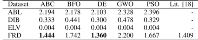
From Table VII, it is further evident that under the present parameter settings, the metaheuristic algorithm DE and ABC performed significantly better than the other metaheuristics algorithms in FIS parameter optimization. Additionally, we found that although the training condition were different in the FIS models IT2FIS-DE, IT2FIS-ABC and IT2FNN-SVR(N), the performance of the IT2FIS-DE and IT2FIS-ABC gave the best training RMSE in comparison to FIS model IT2FNN-SVR(N) [18]. Here, the comparison with literature was limited to only dataset FRD.
TABLE VII
INTERVAL TYPE-2 FISTRAINING RESULTS OVER80%DATA
Dataset ABC BFO DE GWO PSO Lit. [18] ABL 2.194 2.178 2.103 2.328 2.396 -DIB 0.333 0.441 0.300 0.478 0.329 -ELV 0.004 0.004 0.004 0.004 0.004 -FRD 1.444 1.742 1.360 2.200 1.667 1.409 Note:The model Lit. [18] is IT2FNN-SVR(N), which has the best training avg. RMSE among the models listed in Table VI from literature. The dataset FRD had 20% training and 80% test partition.
0 0.5 1 1.5 2 2.5 3 3.5 1 4 7 10 13 16 19 22 25 28 31 34 37 40 43 46 49 52 55 58 61 64 67 70 73 76 79 82 85 88 91 94 97 100 ABC BFO DE GWO PSO
Generation 1 x 100
RMSE
Fig. 3. Convergence of metaheuristics over dataset ABL
Generation 1 x 100 RMSE 0 0.1 0.2 0.3 0.4 0.5 0.6 0.7 0.8 1 4 7 10 13 16 19 22 25 28 31 34 37 40 43 46 49 52 55 58 61 64 67 70 73 76 79 82 85 88 91 94 97 100
ABC BFO DE GWO PSO
Fig. 4. Convergence of metaheuristics over dataset DIB
Generation 1 x 100 RMSE 0 0.001 0.002 0.003 0.004 0.005 0.006 0.007 0.008 1 35 7 9 11 13 15 17 19 21 23 25 27 29 31 33 35 37 39 41 43 45 47 49 51 53 55 57 59 61 63 65 67 69 71
ABC BFO DE GWO PSO
Fig. 5. Convergence of metaheuristics over dataset ELV
Generation 1 x 100 RMSE 0 1 2 3 4 5 6 7 1 4 7 10 13 16 19 22 25 28 31 34 37 40 43 46 49 52 55 58 61 64 67 70 73 76 79 82 85 88 91 94 97 100 ABC BFO DE GWO PSO
Fig. 6. Convergence of metaheuristics over dataset FRD
V. DISCUSSION
We set five dimensions of objectives to explore in the research work (see Section I). To meet with the proposed objectives, first, we presented a concise discussion on the FIS and the metaheuristic algorithms. A detailed discussion on the design of the metaheuristic frameworks is offered in Section III. We explored the use of genetic algorithm (GA) for the optimization of FIS rule-base. In our GA based approach, FIS was formulated into a binary-vector and the population of such binary-vector helped us to optimize the FIS rule-base. We found that for each dataset, GA led FIS rule-base had five rules in its rule-base. The parameters of the obtained FIS (rule-base) were tuned by using different metaheuristic algorithms. We discovered that the FIS optimized using DE gave us the best training and test RMSEs. The developed IT2FISs were tested over four different datasets. The results presented in Table IV, Table V, and Table VII described that the some metaheuristic algorithm performed best in some cases of dataset and some in other datasets (see Section IV). Additionally, a comparison presented in Table VI over the dataset FRD illustrated that the FIS model FIS-DE gave the test RMSE equal to 1.476 and it had performed better in comparison to the other listed FIS models. The convergence analysis presented in experiment phase-II provides us an interesting insight of the FIS training. It described that the longer iterations of training was not very helpful in terms of convergence of the RMSEs since in the most of the cases of datasets, the metahuristics got stuck into local minima at very early iteartion (around 1500-2500). However, some algorithms such as DE and BFO had shown tendency to escape local minima in case of datset ELV (Fig. 5) and datset FRD (Fig. 6). Hence, a carefully setting of metaheuristic parameter offers significant improvement to FIS optimization.
VI. CONCLUSIONS
In this work, supervised training to developed FIS was provided using metaheuristic algorithms. The metaheuristic-based FIS optimization framework had a genotype mapping of the FIS rule base into genetic vector and FIS parameters into a real vector. An optimum rule-base was obtained from a genetic population. Then, several metaheuristic algorithm were applied for the parameter optimization of the obtained FIS. The performances of the FIS and the performances of the metaheuristic algorithms were comprehensively studied. From the performance evaluations, we found that in the training of FIS, which is computationally expensive and which is a difficult optimization problem, the differential evaluation algorithm performed better than the other employed meta-heuristic algorithms. However, the performance of the bacteria foraging optimization algorithm for the test sets were better in some cases. Such performance study was based on the mentioned parameter setting of the metaheuristic algorithms and the programming environment.
ACKNOWLEDGMENT
This work was supported by the IPROCOM Marie Curie initial training network, funded through the People Programme (Marie Curie Actions) of the European Union’s Seventh Framework Programme FP7/2007-2013/ under REA grant agreement No. 316555.
REFERENCES
[1] L. Zadeh, “Fuzzy sets,”Information and Control, vol. 8, no. 3, pp. 338 – 353, 1965.
[2] N. N. Karnik, J. M. Mendel, and Q. Liang, “Type-2 fuzzy logic systems,”
IEEE Transactions on Fuzzy Systems, vol. 7, no. 6, pp. 643–658, 1999. [3] T. Takagi and M. Sugeno, “Fuzzy identification of systems and its applications to modeling and control,”IEEE Transactions on Systems, Man and Cybernetics, no. 1, pp. 116–132, 1985.
[4] H. Hagras, “A hierarchical type-2 fuzzy logic control architecture for autonomous mobile robots,” IEEE Transactions on Fuzzy Systems, vol. 12, no. 4, pp. 524–539, 2004.
[5] D. E. Goldberg and J. H. Holland, “Genetic algorithms and machine learning,”Machine Learning, vol. 3, no. 2, pp. 95–99, Oct 1988. [6] S.-i. Horikawa, T. Furuhashi, and Y. Uchikawa, “On fuzzy modeling
using fuzzy neural networks with the back-propagation algorithm,”IEEE transactions on Neural Networks, vol. 3, no. 5, pp. 801–806, 1992. [7] K. Hirota and W. Pedrycz, “Fuzzy computing for data mining,”
Pro-ceedings of the IEEE, vol. 87, no. 9, pp. 1575–1600, 1999.
[8] D. Karaboga, “An idea based on honey bee swarm for numerical optimization,” Computer Engineering Department, Erciyes University, Tech. Rep. TR06, 2005.
[9] K. M. Passino, “Biomimicry of bacterial foraging for distributed opti-mization and control,”IEEE Control Syst., vol. 22, no. 3, pp. 52–67, Jan 2002.
[10] R. Storn and K. Price, “Differential evolution–a simple and efficient heuristic for global optimization over continuous spaces,” J. Glob. Optim., vol. 11, no. 4, pp. 341–359, Dec 1997.
[11] S. Mirjalili, S. M. Mirjalili, and A. Lewis, “Grey wolf optimizer,”Adv. Eng. Softw., vol. 69, pp. 46–61, 2014.
[12] R. Eberhart and J. Kennedy, “A new optimizer using particle swarm theory,” inProceedings of the Sixth International Symposium on Micro Machine and Human Science, 1995. MHS ’95.,, 1995, pp. 39–43. [13] D. H. Wolpert and W. G. Macready, “No free lunch theorems for
optimization,” IEEE Trans. Evol. Comput., vol. 1, no. 1, pp. 67–82, Apr 1997.
[14] J. G. Carney and P. Cunningham, “Tuning diversity in bagged ensem-bles,”International Journal of Neural Systems, vol. 10, no. 04, pp. 267– 279, 2000.
[15] E. W. Lee, C. P. Lim, R. K. Yuen, and S. Lo, “A hybrid neural network model for noisy data regression,”IEEE Transactions on Systems, Man, and Cybernetics, Part B: Cybernetics, vol. 34, no. 2, pp. 951–960, 2004. [16] J. M. Mendel, “Computing derivatives in interval type-2 fuzzy logic systems,”IEEE Transactions on Fuzzy Systems, vol. 12, no. 1, pp. 84– 98, 2004.
[17] C.-F. Juang and Y.-W. Tsao, “A self-evolving interval type-2 fuzzy neural network with online structure and parameter learning,” IEEE Transactions on Fuzzy Systems, vol. 16, no. 6, pp. 1411–1424, 2008. [18] C.-F. Juang, R.-B. Huang, and W.-Y. Cheng, “An interval type-2
fuzzy-neural network with support-vector regression for noisy regression problems,” IEEE Transactions on Fuzzy Systems, vol. 18, no. 4, pp. 686–699, 2010.
[19] M. A. Sanchez, O. Castillo, and J. R. Castro, “Information granule formation via the concept of uncertainty-based information with interval type-2 fuzzy sets representation and takagi-sugeno-kang consequents optimized with cuckoo search,”Applied Soft Computing, vol. 27, no. C, pp. 602–609, Feb 2015.
[20] O. Castillo, H. Neyoy, J. Soria, P. Melin, and F. Valdez, “A new approach for dynamic fuzzy logic parameter tuning in ant colony optimization and its application in fuzzy control of a mobile robot,” Applied Soft Computing, vol. 28, pp. 150–159, 2015.
[21] O. Castillo and P. Melin, “Optimization of type-2 fuzzy systems based on bio-inspired methods: a concise review,”Information Sciences, vol. 205, pp. 1–19, 2012.
[22] O. Castillo, R. Mart´ınez-Marroqu´ın, P. Melin, F. Valdez, and J. Soria, “Comparative study of bio-inspired algorithms applied to the optimiza-tion of type-1 and type-2 fuzzy controllers for an autonomous mobile robot,”Information sciences, vol. 192, pp. 19–38, 2012.
[23] R. Mart´ınez-Soto, O. Castillo, L. T. Aguilar, and A. Rodriguez, “A hybrid optimization method with pso and ga to automatically design type-1 and type-2 fuzzy logic controllers,” International Journal of Machine Learning and Cybernetics, vol. 6, no. 2, pp. 175–196, 2015. [24] O. Cord´on, F. Gomide, F. Herrera, F. Hoffmann, and L. Magdalena,
“Ten years of genetic fuzzy systems: current framework and new trends,”
Fuzzy Sets and Systems, vol. 1, no. 141, pp. 5–31, 2004.
[25] J. M. Mendel, “On km algorithms for solving type-2 fuzzy set problems,”
IEEE Transactions on Fuzzy Systems, vol. 21, no. 3, pp. 426–446, 2013. [26] H. Ishibuchi, T. Nakashima, and T. Kuroda, “A hybrid fuzzy genetics-based machine learning algorithm: hybridization of michigan approach and pittsburgh approach,” in 1999 IEEE International Conference on Systems, Man, and Cybernetics, 1999. IEEE SMC’99 Conference Pro-ceedings., vol. 1. IEEE, 1999, pp. 296–301.
[27] A. K. Qin, V. L. Huang, and P. N. Suganthan, “Differential evolution algorithm with strategy adaptation for global numerical optimization,”
IEEE Transactions on Evolutionary Computation, vol. 13, no. 2, pp. 398–417, 2009.
[28] C.-F. Juang and C.-T. Lin, “An online self-constructing neural fuzzy inference network and its applications,” IEEE Transactions on Fuzzy Systems, vol. 6, no. 1, pp. 12–32, 1998.