A FRAMEWORK FOR SPATIO-TEMPORAL
TRAJECTORY DATA SEGMENTATION AND QUERY
Huaqiang Kang
A thesis in
The Department of
Electrical and Computer Engineering(ECE)
Presented in Partial Fulfillment of the Requirements For the Degree of Mast of Applied Science(MASc)
Concordia University Montr´eal, Qu´ebec, Canada
March 2019
Concordia University
School of Graduate Studies
This is to certify that the thesis prepared
By: Huaqiang Kang
Entitled: A Framework for Spatio-Temporal Trajectory Data
Seg-mentation and Query
and submitted in partial fulfillment of the requirements for the degree of
Mast of Applied Science(MASc)
complies with the regulations of this University and meets the accepted standards with respect to originality and quality.
Signed by the final examining commitee:
Chair Dr. Wahab Hamou-Ljhad
Examiner Dr. Wahab Hamou-Ljhad
Examiner, External to the Program Dr. Tristan Glatard (CSSE)
Supervisor Dr. Yan Liu
Approved
Dr. William E. Lynch
Chair of Department or Graduate Program Director 20
Dr. Amir Asif Dean,
Abstract
A Framework for Spatio-Temporal Trajectory Data Segmentation and
Query
Huaqiang Kang
Trajectory segmentation is a technique of dividing sequential trajectory data into seg-ments. These segments are building blocks to various applications for big trajectory data. Hence a system framework is essential to support trajectory segment indexing, storage, and query. When the size of segments is beyond the computing capacity of a single processing node, a distributed solution is proposed. In this thesis, a distributed trajectory segmentation framework that includes a greedy-split segmentation method is created. This framework consists of distributed in-memory processing and a cluster of graph storage respectively. For fast trajectory queries, distributed spatial R-tree index of trajectory segments is applied. Using the trajectory indexes, this framework builds queries of segments from in-memory processing and from the graph storage. Based on this segmentation framework, two metrics to measure trajectory similarity and chance of collision are defined. These two metrics are further applied to iden-tify moving groups of trajectories. This study quantitatively evaluates the effects of data partition, parallelism, and data size on the system. The study identifies the bottleneck factors at the data partition stage, and validate two mitigation solutions. The evaluation demonstrates the distributed segmentation method and the system framework scale as the growth of the workload and the size of the parallel cluster.
Acknowledgments
I would like to thank my thesis supervisor Dr. Yan Liu of the Department of Electronic and Computer Engineering. She gave me the chance to focus on what I am interested and pursuit it. It is with her supervision that this work came into existence. For any faults I take full responsibility.
Nobody has been more important to me in the pursuit of my Masters than the members of my family. I also wish to thank my parents for their support both financially and emotionally. Their encouragement and love give me the faith to face the difficulties, whose love and guidance are with me in whatever I pursue.
Finally I would like to thank my friend Zach who encouraged me throughout the time of my research and my life.
Contents
List of Figures viii
List of Tables x 1 Introduction 1 1.1 Problem Statement . . . 1 1.2 Objective . . . 2 1.3 Methodology . . . 3 1.4 Contributions . . . 4 1.5 Thesis Structure . . . 4
2 Background and Related Works 5 2.1 MapReduce Model . . . 5
2.2 NoSQL Database . . . 6
2.2.1 NoSQL Fundamental Concepts . . . 6
2.2.2 Imperfect NoSQL . . . 7
2.3 Open GIS Support . . . 7
2.4 Algorithms and Queries . . . 8
2.4.1 R-tree Building and Query . . . 10
2.4.2 Quad-tree Building and Query . . . 11
2.4.3 DTW for Trajectory Similarity . . . 12
2.5 Spatial Data Storage . . . 14
2.5.1 RDBMS SQL Server 2008 Spatial Indexing . . . 15
2.6 Processing Framework . . . 15
2.6.1 Simba . . . 15
2.6.3 Others . . . 17
2.7 Distributed Parallel Data Analysis System . . . 18
2.7.1 Overview . . . 18
2.7.2 Requirement . . . 18
2.8 Cluster Manager . . . 19
3 On Cloud Data Processing Framework 21 3.1 System Components . . . 21
3.1.1 On Cloud Data Pool . . . 22
3.1.2 Processing Framework Architecture . . . 22
3.2 Trajectory Expression . . . 25
3.3 The Data Model . . . 27
3.3.1 Trajectory Segmentation Methods . . . 28
3.3.2 The Greedy Split Algorithm . . . 29
3.3.3 Parallel and Distributed Implementation . . . 32
3.4 Partition and Indexing . . . 34
3.4.1 Partitioning Techniques . . . 36
3.4.2 Data Shuffling . . . 38
3.4.3 Data Persistence . . . 39
3.4.4 Spatial Indexing . . . 40
3.4.5 Local R-tree Indexing . . . 40
3.5 The Query Workflow . . . 42
3.5.1 The Parallel Intersection Join . . . 43
3.5.2 In-memory Query . . . 44
3.5.3 On Graph Store Query . . . 46
3.5.4 Duplication Elimination . . . 46
3.5.5 Raw Data Separation Technique . . . 46
4 Trajectory Metrics 47 4.1 Trajectory Similarity Estimation . . . 47
4.2 Collision Detection Metric . . . 50
4.3 An Evaluation Application . . . 54
4.3.1 Graph Build Up . . . 54
4.3.3 Test Dataset . . . 56
4.3.4 Existing Gathering Implementation . . . 56
4.3.5 Small Size Trajectory Analytics . . . 56
4.3.6 Medium Size Trajectory Analytics . . . 57
4.3.7 Trajectory Transforming to MBR Visualization . . . 59
5 System Performance Evaluation 60 5.1 The Experiment Setup . . . 61
5.2 Evaluations on In-memory Framework Based on GeoSpark . . . 62
5.2.1 Cluster and Partition Size Efffect . . . 62
5.2.2 Data Size Effect . . . 65
6 Discussion 71 6.1 Data Skew Analysis . . . 71
6.2 Replacing Partitioning Strategy . . . 71
6.3 Introducing Time Dimension When Partitioning . . . 74
6.4 Unaddressed Problems . . . 76 6.5 Reliability Factors . . . 76 6.6 Threads to Validity . . . 76 7 Conclusion 78 Appendices 80 A System Deployment 81
List of Figures
1 How Map Reduce works . . . 6
2 JTS UML Chart . . . 8
3 Modelling Object Interactions. [7] . . . 9
4 An R-tree Structure [2] . . . 13
5 SQL Server Indexing [1] . . . 16
6 Overview of YARN Architecture [34] . . . 20
7 Overview of Framework Architecture . . . 23
8 The Trajectory MBR in 3-D. [9] . . . 26
9 Data Model of Trajectory Segmentation . . . 27
10 Main Steps of the Greedy Splitting Process . . . 30
11 Framework Workflows . . . 35
12 Dataflow Between Nodes . . . 36
13 The Neo4j Local R-tree Visualization. . . 41
14 The Trajectory Query Workflow in Two Parallel Partitions. . . 43
15 Similarity Estimation Metric in 2D . . . 50
16 The Illustration of Three Blue Checkpoints for Collision Detection . . 52
17 The Connected Components(Crowds) in Graph Database . . . 55
18 Positive Crowd Pair Trajectories Snapshot . . . 58
19 The Heat Map of Trajectories and MBRs . . . 59
20 Speedup under Different Cluster Size . . . 63
21 Throughput under Different Repartition Numbers . . . 64
22 GeoSpark 8 Node Clustering . . . 65
23 GeoSpark 16 Node Clustering . . . 66
24 Throughput under Different Data Size . . . 66
25 Throughput under Different Segments per Trajectory . . . 67
27 Segmentation Repartition Shuffling Ratio . . . 69
28 Graph Database Based Framework Latency Decomposition . . . 70
29 Neo4j 16 Node Clustering . . . 70
List of Tables
1 Comparison Between Different Spatial Processing Frameworks. . . 17
2 Frequently Used Notations. . . 26
3 Confusion Matrix for Gathering Detection Result,a total of 3330
Tra-jectories . . . 58
4 Confusion Matrix for Positive Detected 2740 Trajectories as Input . . 58
Chapter 1
Introduction
With the fast development in micro-electronics, increasing location tracking equip-ment is facilitated in transportation, personal health and public security fields. GPS tracking systems have been applied to collecting data of wearable devices, vehicles to study their behaviors, track vehicle’s routes, and produce diverse applications in-cluding points of interests, recommendation, health monitoring safety regulation, and fleet management.
1.1
Problem Statement
GPS raw data are usually recorded as spatio-temporal points. For example, an IMU sensor [32] applied to automotive car produces ten records per second, with each record of at least 20 Bytes. For every hour each car on the road, the IMU sensor gen-erates 36,000 records with the size of over 700MB [70]. As the scale of managed cars expands dramatically, the trajectory data becomes a source of Big Data. Processing of trajectory data timely or in real-time inherits Big Data challenges.[61] When the data size is beyond the capacity of a single processing node or the processing latency has a higher requirement shorter than a single node processing time, the trajectory data are required to be distributed and processed in more salable multiple nodes. [29] [30]
For self-join query operation, the time complexity is O(N2). Partitioning the data
site into smaller set can significantly reduce the time cost of each single query. Should the framework distribute the data based on file objects or based on geolocation? If geolocation partitioning is considered, which strategy is the best practice to handle
the data density varying from urban to rural? [16]
After data are distributed, how to express the trajectories is a big challenge. Is there any possibility to transform a set of points into more efficient geometry shapes? How the system organizes the shapes and utilizes any index to optimize the queries is another challenge. After the transformation, to what extent of the shape characteristic of the trajectory is preserved during trajectory similarity search? Based on the index and segmentation, there should be an algorithm to evaluate the trajectory similarity and finding the most one out. [23] [42]
In this thesis, the study focuses on three research questions of distributed parallel processing of trajectory segmentation.
R1: How to partition and segment trajectories in a distributed framework?
R2: What are the key factors of parallelism that affect the scalability of
trajec-tory segmentation and queries?
R3: When trajectory segments are queried for analysis, how much performance
the result gains in cluster processing compared to the single node processing of trajectories.
1.2
Objective
The objective of this thesis is to develop a framework that can parallel process the trajectory into segments and distribute the trajectories into multiple nodes using data partitioning strategies. The load and transformation should be parallel to increase the efficiency. There should also be a parallel trajectory query framework that enables intersection query to get the desired trajectory results. The framework should ensure the low latency in the streaming processing scenario and it can also adapt to the data warehouse’s large quantity of data case. The framework can be elastic to adapt to the size of data to be processed and the latency requirement.
Furthermore, trajectory metrics could be developed based on these queries for further analysis model. Last but not least, we should have a story in real data to demonstrate the ease of use in this framework and track down the bottleneck and data skew of the system to avoid this when put it into practice.
1.3
Methodology
In this thesis, it requires a parallel trajectory segmentation method that scales hor-izontally as the size of the trajectory data, the load of queries and the number of worker nodes grow. This method consists of a split algorithm for parallel trajectory partition and workflows for queries of segments for trajectory analysis. This work-flow is to be implemented to investigate the parallelism factors of scalability using two frameworks, one is distributed in-memory processing and the other is NoSQL graph storage. Spatial indexes and query operations in each framework are built.
To realize this workflow, this study further requires a data model for representing trajectory segments and associated geometric operations. A long trajectory should be transformed into small segments and then being warped with Minimum Bounding Rectangles(MBRs). For the lowest latency, the MBRs as well as the indexes of the MBRs is going to be stored in each cluster node’s memory. On the other hands, when the data exceed the size of cluster memory,geometric objects are indexed and stored in a NoSQL graph database as an alternative.
To demonstrate the usage of the proposed method, two metrics that are integral to applications such as trajectory clustering analysis are defined. One metric esti-mates the similarity of trajectories. This study also defines a threshold of Euclidean distances of trajectories to count if any moving objects are within this threshold at a certain period. The other metric detects the collision chance by measuring the intersections of two trajectories.
This research evaluates the method proposed by two means, (1) system-level per-formance evaluation and (2)comparison of results from the trajectory clustering work-flow with another clustering method. For the system level performance evaluation, workflows on the Amazon Elastic MapReduce (EMR) platform are developed. The trajectory data are from Microsoft GeoLife [74] data with the size of 1.6GB and 24 million moving object records. The experiments show the performance on GeoSpark has an improvement speedup ranging from 2 to 2.5 with 8 node cluster or 16 cluster compared with the single node system. The evaluation on Neo4j framework has a maximum speedup of 17.5 times improvement when expanding the cluster size from 1 node to 16. In term of accuracy of clustering results, it reaches 87.2% accuracy compared to GPFinder [68] as ground truth.
geographic imbalance. A dynamic partitioning method to adjust each partition’s load of objects is adopted. Furtherly a data skew mitigation solution by involving other non-geographical property as secondary key when distributing data is devised.
1.4
Contributions
The main contribution of the thesis is four-fold. The implementation is accessible
from Github-https://github.com/kanghq/SparkApp [31].
1. We firstly apply the Greedy-Split trajectory segmentation algorithmwith
MapRe-duceprogramming model on a distributed system;
2. A system workflow that queries trajectories segments in-memory and in a
graph databaseis developed. Integration indexing techniques for fast queries is also performed.
3. This study defines metrics that are further utilized by applications such as
trajectory clustering analysis
4. A data skew migration solution is developed to balance the workload as both the size of the data and the computing cluster grow.
1.5
Thesis Structure
The thesis follows this structure:
Chapter 2 introduces the related works of trajectory segmentation, storage, and
access.
Chapter 3 presents the framework system architecture, segmentation, indexing
and query flow.
Chapter 4 illustrates a real life use case for evaluating.
Chapter 5 shows the experiments results.
Chapter 2
Background and Related Works
2.1
MapReduce Model
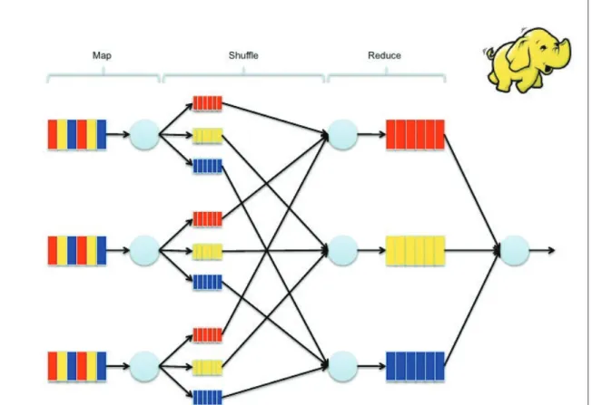
Previously, the parallel computing is restricted to parallel algorithms. Traditional parallel algorithms include dense matrix algorithms, sorting, graph algorithm, search algorithms, dynamic programming, and fast Fourier transform [36]. This limits the usage of high-performance parallel computers. In 2008, Google proposed MapReduce programming model to make it possible for large datasets in parallel processing.
This model can be described in five stages.1) mapping input as <Key, Value> pair.
2) computing on single <Key, Value> record. 3) grouping intermediate data. 4)
computing on intermediate data. 5) reducing for final result. Figure 1 gives an
intuitive impression on MapReduce model.
MapReduce provides a simple and universal parallel programming model. How-ever, there are also cons. There are a large number of algorithms can not be rewritten to MapReduce model. Not like SQL, it is a lower level language. You have to focus on how to retrieve data and how to sort these. Recently, there are some middlewares like Hive [70] providing similar SQL language to manipulate data as well as the indexing support. Another drawback is its low efficiency. It enables only single dataflow in the whole framework. The stages between map and reduce are block operations. The shuffling stage consuming large of I/O also needs attention when programming.
Figure 1: How Map Reduce works
2.2
NoSQL Database
2.2.1
NoSQL Fundamental Concepts
NoSQL or Not Only SQL database emerges at the background of big data analy-sis. The appearance of NoSQL databases aims to solve the following weakness that traditional RDBMS can not handle.
Here are the motivations of creating NoSQL databases [59]:
To avoid unnecessary ACID complexity;
Giving high throughput in big data analysis;
Ability of horizontal expatiation on non-dedicated servers;
More flexibility than database norms;
2.2.2
Imperfect NoSQL
NoSQL is not a replacement of DBMS. However, it is more an alternative when the data are more flexible where it is hard to fit for the RDBMS. In traditional RDBMS, all data fields should be defined property with constraints. RDBMS can provide the maximum robust data integrity. The simple SQL query method makes optimization easy and reliable.
For this system, the choice of graph database gives the system more flexibility in the query of graph theory algorithms. For example, as a graph database, Neo4j
pro-vides some path finding algorithms, community detection like Louvain algorithm [6]
orconnected components algorithm.
2.3
Open GIS Support
Spatial topology refers to the relationship between spatial objects. Applying topology in a GIS system has three benefits.
Topology is necessary for route planning. Without topology, it is impossible to
route to a certain destination via the road network.
Topology can be used to validate data for better data quality. For example,
a utility hole should be outside polygon objects where the shape of roads are represented.
By creating the topology relationship between features and objects, it is possible
to synchronize the features to make them consistent.
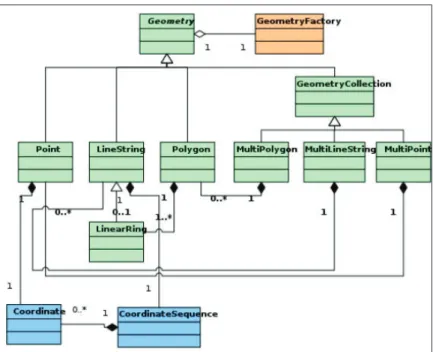
This framework imports a third party library to support spatial topology called
JTS Topology Suit. It’s a group of core APIs for processing geometry. The UML chart is shown in Figure 2 [14]. With JTS library, it is possible to read standard WKT or WKT format shapes, building indexes, to query desirable objects and to compute metrics.
It has complete 2-D linear geometry model supporting Point, LineString,
Lin-earRing, Polygon, MultiPoint, MultiLineString, MultiPolygon, GeometryCollection. JTS follows OpenGIS API standards, and follows Dimensionally Extended nine-Intersection Model(DE-9IM) [60], which means you can compute the spatial
Figure 2: JTS UML Chart
crosses, overlaps, covers, coveredBy. These 9 intersection relationships are shown in Figure 3.
There are four overlay methods in JTS. They are intersection, union, difference,
symmetric difference as heterogeneous overlay.
The precision Model provides floating and fixed coordinate models. It can give different capacities putting points in the grid.
JTS also provides the metrics to measure the spatial objects including area, length, distance, WithinDistance and Hausdorff Distance.
The supported spatial indexes are Quadtree,StRtree, kD-tree, Bintree, Mono-toneChains, and SweepLine.
2.4
Algorithms and Queries
Trajectories need to be simplified by cutting into smaller, less complex primitives. Anagnostopoulos et al. [4] illustrate a method of segmentation that adapts to Nearest-Neighbor search and analyzes the segmentation problem in a global view. Cudre-Ma uroux et al. [13] give a solution for large size of trajectories on disk. They maintain an optimal index and the data are dynamically co-located. To reduce the I/O, the system also adapts to queries for optimization. Mokbel et al. [45] show us three major
Figure 3: Modelling Object Interactions. [7]
spatio-temporal access methods, namely “Indexing the Past”, “Indexing the Current Positions” and “Indexing the Current and Future Positions”. The mostly used one is indexing the past positions, such as STR-tree or RT-tree [27]. Another method commonly used is to index the current positions, such as LUR-tree [37] and Hashing. The third method of indexing is to index the current and future positions, including PMR-quadtree [49] and SV-Model [11]. A new trend of accessing trajectories is using parametric rectangles [11]. They do not enclosure the trajectories directly; they create the bounding rectangles as a function of time. The moving objects would be in the
same rectangles for a time instance t.
For motion classification, Fu et al. proposed a similarity-based pattern grouping method compared with fuzzy K-means [24]. Giannotti et al. [25] also presented two purely temporal trajectory pattern mining approaches. They firstly transform the sequences of points into regions of interest. Then they use origin-destination matrices
to find out pre-conceived regions or used a dense based discretization method to find out the popular regions. The authors Panagiotakis et al. [52] introduce a methodology to find out the most representative sub-trajectories. They represent the trajectories based on multiple attributes and then sampled them without supervision.
2.4.1
R-tree Building and Query
R-tree is widely used both in partitioning technique and indexing method. R-tree is a depth-balanced tree, so the root should have at least two children to be balanced.
The children number of a node (except leaf or root) is between m and M, where
m∈[0, M/2]. M is the max number of children of a node. The depthd of an R-tree:
logmN −1< d <logMN −1 .
Algorithm 2 gives an examplequery(root,q)to find objectqfrom root of R-tree.
Algorithm 1 Algorithm for R-tree Query query(u,r)
Input: a query object r wrapped by MBR mbrr, search root entry u.
Output: objects overlapped with r.
1: if u is a leaf then
2: return all objects overlapped with r
3: else
4: for each each child v in node u do
5: if mbrv overlapped with r then
6: query(v,r)
7: end if
8: end for
9: end if
The time complexity of search can be considered into two conditions: 1) if
Bound-ing boxes do not overlap the query objectq, the complexity isO(logmN). in the worst
case, when all objects’ bounding boxes are overlapping on q, it is O(N) [63].
Given an object p to be inserted, the study illustrates the insert(root, p)
al-gorithm to show how R-tree is built.
For thechoose-subtree(u,p)function in Algorithm 3, the aim of this function is
Algorithm 2 Algorithm for R-tree Insertion insert(u,p)
Input: a new object p wrapped by MBRmbrp, R-tree root entry u.
1: if u is a leaf then 2: add pin node u 3: if u overflows then 4: handle-overflow(u) 5: end if 6: else 7: v := choose-subtree(u,p) 8: insert(v,p) 9: end if
its capacity during the inserting, it triggers handle-overflow shown in Algorithm 4 to split one node into two to ensure the tree is balanced.
Algorithm 3 Algorithm for R-tree sub tree choosing choose-subtree(u,p)
Input: root entry u, new object pto be inserted.
Output: the
1: for vi as one of the child of root udo
2: voli := volume(mbrv+p - mbrv)
3: end for
4: get the smallest volk
5: return vk
Algorithm 5 illustrates the split operation in R-tree.
For a good split solution, there are two standards to evaluate it. 1) the total area of the two nodes is minimized and the overlapping of the two nodes is minimized.
Study shows that the complicity of finding an optimized split solution is O(2M+1).
Figure 4 is a typical R-tree structure, where M = 3 , m = 2.
2.4.2
Quad-tree Building and Query
Quad-tree is another hierarchical spatial data structure. It is a rooted tree and each node has a fixed number of 4 children. Each node expresses a square area in the space and each child of this node expresses one quadrant of the space. It’s a non-balanced tree and can be used to express non-uniform meshes. Algorithm 6 shows how to insert
a point p from a Quad-Tree with insert(root, p) function. From the algorithm, each
Algorithm 4 Algorithm for R-tree overflow handling handle-overflow(u)
Input: root entry u.
1: split(u) into two parts u and u
2: if u is the root then
3: create a new root and connecting u and u
4: else
5: w:= parent(u)
6: update w := new MBR(u)
7: add new child u to w
8: if w overflows then
9: handle-overflow(w)
10: end if
11: end if
Algorithm 5 Algorithm for R-tree split split(u)
Input: root entry u, parameterβ ≥3 .
Output: two new child MBRs mbrs1 and mbrs2 covering u
1: m := size of objects in u
2: sort objects under u in x-dimension
3: for i := 0.4βto m− 0.4βdo
4: S1 := first i objects in list
5: S2 := the other iobjects in list
6: get mbrS1 and mbrS2
7: end for
8: repeat 2-6 line with the respect of another dimension
9: return mbrS1 and mbrS2 with the best solution
together. The depth of a Quad-tree
d=log(s/c) + 3/2
wheres is the initial square length andcis the smallest distance between two points.
It hasO((d+ 1)n) nodes and the construction time complexity isO((d+ 1)n) too [46].
In the case of rectangles, it is resembled that the point as zero height zero width polygon. During the insertion, it should make sure each cell is not big enough to fit the whole polygon and the polygon does not need to be stored in the leaf node.
2.4.3
DTW for Trajectory Similarity
Dynamic Time Wrapping (DTW) [5] algorithm is firstly introduced for speech recog-nition. Then it is used to time series analysis applications. It can be used to compare
Figure 4: An R-tree Structure [2]
two trajectories with different length. To find out the mating points, the pairwise Eu-clidean distance matrix should be prepared first. A path satisfies ”monotonic” and ”continuity” from bottom left to top right makes the alignment between sampling nodes.
It should be noticed that the DTW algorithm only compares the sampled ”points”, not the trajectory. So the GPS sampling interval or video stream frame rate may interfere the accuracy between two trajectories. Also, DTW origins from time series algorithms, which lacks the consideration of temporal attribute [43].
Algorithm 6 Algorithm for Quad-Tree Construction insert(u,p)
Input: root entry u, point to be inserted p
1: if u’s boundary not contain p then
2: return false 3: end if 4: if v is empty then 5: add pto cell v 6: return true 7: else
8: subdivide N W, N E, SW, SE four quadrants
9: if insert(NW,p)then 10: return true 11: end if 12: if insert(NE,p) then 13: return true 14: end if 15: if insert(SE,p) then 16: return true 17: end if 18: if insert(SW,p) then 19: return true 20: end if 21: return false 22: end if
2.5
Spatial Data Storage
Most geological data are based on geometry. The most common method is to use traditional RDBMS as column wise store. For the geographical data, there are two ways for storage. The first one is raster-based and the second one is vector-based [66]. The object is represented as a series of lines connected to form a polygon. The RDBMS can easily store the coordinates of vertices. In the raster-based system, the real world object is formatted by cells and represented as a series of contiguous cells. ESRI company develops a spatial database engine providing the middle layer to store GIS data in RDBMS like DB2, SQL Server or Oracle. It is also popular to use geometry database to store this geological information. DISASTER [73] is a Portuguese GIS database based on the most popular open source MySQL database engine. It stored floods and landslides for the period of the year 1865 to the year 2010. In [40], they have developed mechanisms to integrate multiple data sources and finally
a seamless database was achieved. A data warehouse supporting streaming data was designed [51]. The data warehouse supports trajectory properties such as average velocity, maximum acceleration as well as aggregation operations.
2.5.1
RDBMS SQL Server 2008 Spatial Indexing
This study uses SQL Server as an example to introduce how traditional database handles spatial data. SQL Server has built-in geometry support. “GEOMETRY” and “GEOGRAPHY” types express points, lines, polygons or multi-polygons. The expression format can be Well-Known Text (WKT), Well-Known Binary (WKB) as well as GML [12].
In traditional RDBMS like SQL Server, it utilizes B-tree to achieve the support of 2-dimensional spatial data. The entire space is decomposed into a grid hierarchy. The cells are numbered in Hibert space-filling curve. There are four levels grid hierarchy
and each level can be configured as HIGH, MEDIUM or LOW density divisions to
decide the density of cells per layer. If a cell is contained in an object, it is not tessellated further. If an object is covered by multiple cells, the database records these cells respectively. Figure 5 is an example of SQL Server indexing [20].
2.6
Processing Framework
For distributed spatial analytic systems, they can be divided into two camps. The one is Hadoop based systems that store the intermediate data in the shared disk system. The other one is Spark based, which processes data in memory only.
2.6.1
Simba
Simba [69] is a new distributed spatial processing framework. Most of its operations are based on native Spark APIs. It extends the query features with the support of
SQL statements. Multiple varieties of space operations like kNN Query, kNN join
distant join are supported in this framework. It reconstructs the fundamental RDD
architecture to IndexRDD. It is possible to have the indexes persisted on disk and
loaded back but it does not support full data disk persistence.
Figure 5: SQL Server Indexing [1]
planer, SQL can be used as input and the optimizer in SQL planer can make the best
use of existing indexes and statistics. This planer is based on optimization rules and
cost-based optimizations.
Simba has two-level indexing strategy. The first level index gives quick access to the partition where the spatial object belongs; the second level R-tree indexes optimize the spacial operations like range query, kNN join or distance join. Simba supports concurrent query execution by deploying a thread pool in the query engine. This is a platform level concurrency strategy that does not need the involvement of users.
As a cluster based system, Simba has the ability of fault tolerance inherited from Spark. When a master fails in the multiple masters environment, recovery mechanism ensures the global indexes are not missing. Also the query job in Simba triggering Spark transformation job can be guaranteed to recover from failure with the help of
Spark native design.
2.6.2
SpatialHadoop
SpatialHadoop [15] is another distributed processing framework based on Hadoop. It provides native support of spatial data. Not like Hadoop-GIS [3] treats the Hadoop
framework as a black box; Spatial Hadoop realizesrange query,kNN query, andspatial
join functions which enable the user to develop a higher level application.
In SpatialHadoop, there are four layers: language layer, operation layer,
MapReduce layer, and storage layer. In language layer, SpatialHadoop sup-ports SQL-like scripting by applying Pig Latin [50] extension. To support spatial data, Pegeon [17] is also integrated into SpatialHadoop. Casual users can directly do Ad-hoc query with SQL-like scripts. In Operation layer, the spatial operations are encapsulated for developer use. Higher level functions can be expanded in SQL-like
scripts. In MapReduce layer, SpatialHadoop involves SpatialFileSplitter to split
in-put file by blocks so that the indexes can be built up efficiently. SpatialRecordReader
transforms spatial data into key-value pairs, extracts indexes and sends the spatial data to map function in blocks. Lastly, the storage layer provides grid partition file storage and R-tree or R+-tree support. It archives up to 4.6 TB data processing in the prototype test.
2.6.3
Others
LocationSpark [62] and Magellan [58] are both spatial data processing extensions based on Spark. They provide multiple partition techniques, indexes and multiple query methods such as range query, KNN or spatial join. Table 1 lists the features of different frameworks.
Table 1: Comparison Between Different Spatial Processing Frameworks.
Features GeoSpark Simba SpatialHadoop Magellan LocationSpark This Framework
Data Dimensions 2 Multiple 2 2 2 3
Spatial Indexing R-tree/Quad-tree R-tree Grid/R-tree ZOrderCurves Grid/R-tree/Quad-tree R-tree
In-memory Yes Yes No Yes Yes Yes
SQL No Yes Yes No Yes No
2.7
Distributed Parallel Data Analysis System
2.7.1
Overview
While data size exceeds the capacity of a single machine, especially in today’s Web 2.0 era, a new way to share the resource between multiple computing nodes are required.
Distributed computingconsists of software components, hardware components as well as network components. Compared to the centralized system, there are many benefits that distributed system can offer:
Scalability: a centralized system can be limited by the microelectronics to
in-crease the capacity or power to boost the scalability of a system. The distributed system scalability can be easily expanded by adding more computing nodes as required.
Redundancy: centralized system reserves all the resources in the server. When
the central server is unavailable, the whole system is down. Distributed system can duplicate the data into multiple copies to ensure more accessibility and avoid single node failure.
Price/performance ratio: since many smaller machines can be used to scale out,
the total cost is lower than one powerful machine.
2.7.2
Requirement
The design of a distributed system should achieve the following goals:
Openness: the communication protocols or infrastructures should be easy to
access, which will make it easier for troubleshooting in a large scale distributed system.
Transparency: The framework designed should conceal heterogeneous
architec-ture. The fact that the resources are distributed across the network and should provide a universal way of retrieving the resources even though the resources are relocated or part of the system is in a failure status.
Scalability: A scalable distributed system is a system that can be flexible with
2.8
Cluster Manager
In this cloud distributed system, Yarn is selected as the cluster manager. Yarn [65] is a resource manager for scheduling jobs and monitoring the CPU, memory, disk and network usage. There are two components called Resource Manager(RM) and Node Manager(NM). Between the Resource Manager and Node Manager, there is a frame specific Application Master(AM) which is responsible for negotiating with RM and NM. The NM is responsible for nodes and responds to the requests from RM. RM is the interface accepting jobs from clients and schedules it. The manager communication between nodes uses RPC service [48]. The whole architecture of YARN can be found in Figure 6.
To execute a distributed job. There are several steps happening in the cluster : 1. Client decides which input data is required for execution and fetches its
meta-data.
2. Client generates descriptor HDFS files that contains the location of each parti-tion.
3. Client triggers AM and RM.
4. AM negotiates resource containers with a set of nodes. 5. Application executes in the container.
Chapter 3
On Cloud Data Processing
Framework
3.1
System Components
The system designed has the following key components.
Data Pool: Data pool is the source of data to be processed. It can be from other OLTP databases, some offline wearable devices, offline storage drives like tape drives or any other distributed file system such as HDFS.
Processing Framework: This thesis uses Spark as the processing framework. Inside Spark, Remote Procedure Call (RPC) and event loop mechanisms are used to communicate with each other. There is a subsystem called Netty achieving these. For bulk data transportation like shuffling, Spark uses Java Non-blocking I/O (NIO) to transfer the data. There is also some broadcast data transportation delivered by Jetty [33] subsystem. As an extent to the spatial field, Java Topology Suit (JTS) is selected as the GIS format data support.
Distributed System Management Software: To sufficiently manage these
resources and to schedule tasks, Yarn a cluster manager is introduced to track these resources. This component will be explained in the following section.
Distributed Persistent Software: In this system, two persistent methods are used, one is an in-memory method based on Spark native RDD, another one is based on graph-database implemented by Neo4j.
3.1.1
On Cloud Data Pool
In this system, Amazon S3 is selected to store the raw dataset gathered from the Internet.
Amazon S3 stands for Simple Storage Service. As an object storage system, it mostly is used for backup and restore, disaster recovery, archive, data lakes and big data analytics, hybrid cloud storage or cloud application data storage. As an object storage service, it can ensure 11 9’s durability and 99.99% availability.
To use the S3 storage, users are required to create a bucket in a specific region. Then it is possible to use API like REST API or SOAP interface to upload objects into buckets. Each object consists of object data and metadata. An object can be identified by a key in the bucket and a version ID. Amazon S3 provides eventual consistency when multiple clients are writing at the same items.
3.1.2
Processing Framework Architecture
Apache Spark[72] is an In-memory computing framework based on the MapReduce programming model. It has multiple extension modules such as streaming comput-ing, machine learncomput-ing, graph theory, or SQL support. Spark is written in Scala but supports multiple languages including Python and Java. Resilient Distributed Dataset(RDD) is the primary storage structure in Spark. All computation operations
on the dataset are the transormations towards RDDs.
RDD is cacheable and fault-tolerant. If one or more partitions are missing or failed, Spark can restore from the data source with the help of lineage transformation
plan. RDDs are read-only. There are two ways of creating an RDD: parallelizing
existing in-memory collection or referencing a dataset from external storage.
For a better optimization, Spark transforms RDD lineage into Directed Acyclic Graph(DAG) stages. The stage is the minimal schedule unit. It applies lazy load technique which means the stages are not executed until an action in the workflow requiring the results to produce non-RDD values.
Previous frameworks store the intermediate data on disk like HDFS, so the next task can retrieve the shared data from there. Spark provides a new approach to enable the intermediate data stored in memory and shared between nodes for parallel computing.
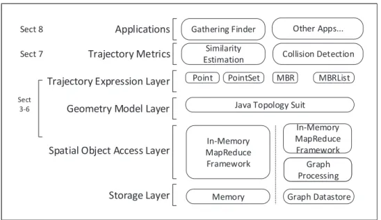
The framework architecture follows a layered architecture to support metrics cal-culation, topology modeling, parallel distributive processing, query, and storage. The architecture is shown in Figure 7.
Point PointSet MBR MBRList Java Topology Suit
Gathering Finder Other Apps...
Graph Processing Graph Processing In-Memory MapReduce Framework Similarity
Estimation Collision Detection
In-Memory MapReduce Framework
Memory Graph Datastore Sect 8
Sect 7
Trajectory Expression Layer Geometry Model Layer
Spatial Object Access Layer
Storage Layer Trajectory Metrics Applications
Sect 3-6
Figure 7: Overview of Framework Architecture
Application Layer
The first layer is theApplication Layer. All applications that utilize trajectory metrics
are defined to exist in this layer.
Middle-ware Layers
The second layer is the Trajectory Metric layer. In this layer, all trajectory metrics
are calculated. Three dimensions are considered in the system, namely time, latitude and longitude. The topology calculation results are further processed as numeric metrics.
The third layer is the Trajectory Expression Layer, where the raw GPS coordinate
data are generated into trajectory segments. The raw spatio-temporal data generated from portable devices are loaded in the system in a batch mode. At this layer, each
trajectory data are converted toPoint objects in the data model of Figure 7. And then
the trajectories are further processed as rectangles shape called Minimum Boundary Rectangles (MBRs). The further discussion about MBR is elaborated in the next section.
The fourth layer is the Geometry Model Layer. At this layer, topology calculation is performed. It converts MBR objects to JTS objects. The benefit of converting to JTS objects is that the trajectory metrics relying on geometric calculating operations on MBRs are supported by JTS library, such as spatial predicates, convex hull, and metric calculation referred in Section 4.3.
Infrastructure Layers
The fifth layer is the Spatial Object Access Layer. The operations on MBRs are
specific to the data processing frameworks. In this thesis, two kinds of data processing frameworks are considered, namely a NoSQL graph database and Apache Spark in-memory processing framework. If MBRs are stored in a graph processing system (such as Neo4j), Cypher, a graph query language is programmed to operate these data. If the MBRs are operated by an in-memory geometry processing framework(such as GeoSpark [71]), Spark parallel functions to access MBRs are developed.
The sixth layer isstorage layer. In the graph processing system, MBRs are indexed
and stored in the directed graph structure. They are distributed on multiple database nodes. For the in-memory processing framework, MBRs are indexed and stored in a customized tree structure. The tree structure is organized in Spark RDD structure for distributing.
3.2
Trajectory Expression
Trajectories can be collected from various types of devices. The most commonly seen trajectory data are collected from GPS tracker. A GPS tracker periodically receives the signals from GPS satellites and calculates the current position. This requires the device to be exploded to an open area to receive signals. For indoor trajectory collection, GSM cell stations, WI-FI hot spots or RFID labels are used to get the approximate current location. Furthermore, the trajectories can also be extracted from video stream file like surveillance cameras.
A trajectory is a collection of unique points organized in time series order. For the
unprocessed data, this thesis uses T r =< pt1, pt2, ..., ptn > to express a trajectory.
A point can be expressed with four elements: ptk = (idk, lock, tk, Ak) in kth position.
idk is the position identifier; lock is the spatial location of the position; tk is the
time at which the position was recorded; Ak is the additional data like altitude or
temperature. For lock, it can be expressed as coordinate data (x, y) if the data is
collected from GPS-based device or the lock will be marked as the cell ID of a GSM
base station, Wi-Fi hot spot, or an RFID label. If the location is marked by cell ID, these data should be transformed into coordinates so that they can be expressed in Euclidean space.
Further more, the trajectory can be simplified as a rectangle or an envelope formed by the minimum and maximum latitude and longitude coordinate. The rectangle is
calledMinimum Bounding Rectangle (MBR). The MBR is an approximation of
the trajectories and that transforms the discrete point problem into topology problem. Figure 8 shows how an MBR bounding a trajectory in 3 dimensions.
In this project, the trajectory files generated by GeoLife devices are GPS position logs. Each trajectory is a single “plt” file. It records the latitude, longitude, altitude in feet, data and time. The framework firstly loads the data in bulk from Amazon S3
datastore. Then it parses each single ptk into Point datatype and a sub trajectory
T r can be expressed as a PointSet datatype.
A segmentation method splits one trajectory into maximal K segments. In this
thesis, segments are the first class entities for indexing, storage, and query. In this segmentation method, a data model with components to encapsulate the operations on segments is designed. Then a greedy split algorithm to split each trajectory into segments is presented. Since trajectories are independent, this greedy-split method is
Figure 8: The Trajectory MBR in 3-D. [9]
processed in parallel. The commonly used notations in this thesis is listed in Table 2. Table 2: Frequently Used Notations.
Notation Meanning
T rp (resp. T rr) a trajectory p (resp.r)
mbru,T rp,i
an MBR in trajectory T rp, sequencei,
partition u , K ∈N, k∈[1, K], K is the
maxi-mum segmentation number of one trajectory
ptT rp,i a GPS coordinate point in trajectory
T rp, sequence i, pt∈T r
pt.x coordinate longitude
pt.y coordinate latitude
Rc,v(resp.Rq,u) Candidate MBR relation, partitionv
(resp. query MBR, partition u)
Est(T rp, T rr) Trajectory similarity estimation
between T rp and T rr
3.3
The Data Model
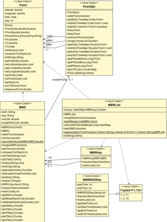
The data model’s entities and their relationships are presented in Figure 9.
Figure 9: Data Model of Trajectory Segmentation
Point. Since the GPS trajectories are described as spatio-temporal points, the
models or topology, they mostly support only 2-D attributes of longitude as X and
latitude as Y. This framework supports an extra attribute of the timestamp T. Ours
also supports the Euclidean distance calculation when required.
PointSet. A trajectory consists of a cluster of points as time elapses. PointSet
class to express the sub-trajectories is created. At least one point can be the smallest sub-trajectory. These sub-trajectories can be linked to form a longer sub-trajectory
by using addAll() function or only adding one point to extend this trajectory. All
these internal points have their sequence order by sorting their timestamps.
To get one position snapshot at a specific time, this framework uses the func-tion getPtSnp(). As an estimation in between two real points, a virtual position is calculated based on the average velocity between the two adjacent positions.
Minimum Boundary Rectangle (MBR). The MBR class focuses on the
at-tributes that relate to operations on trajectory segments such as the volume and merging cost in the greedy-split algorithm. The merge procedure will be presented in detail in this section later. Since an MBR covers a sub-trajectory, it is a composition
made from this sub-trajectory’s PointSetand this MBR’s four vertexes. The
frame-work can get the MBR vertexes of its sub-trajectory by using the range() function
and get its volume by using volume()function.
MBRList. The MBRList is a data structure to organize the MBRs in a linked
list. The attributeMBRKey is used in theMBRList for queries.
3.3.1
Trajectory Segmentation Methods
Dieter Pfoser et al. [53] compare several query approaches of moving objects. The naive way is to query the sampled points directly. Using the coordinate-based query such as nearest-neighbor, range query is possible. It can not reflect all the movement of the objects especially for the times in-between the sampled points. Further, the linear interpolation can be used. the algorithm connects the points as endpoints of segments. The queries are trajectory-based topological queries which can handle speed, acceleration information or more.
In this system, it puts the sub-trajectories into Minimum Bounding Rectangles (MBRs). MBRs can simplify the topology query and as an approximation spatial query as well as for spatial indexing propose.
homogeneous pieces. A high standard trajectory segment can expose clear informa-tion in high level representainforma-tion, reduce the chance of noise and finally give a bet-ter expression for the algorithm to analyze the behavior behind the trajectories [10]. The commonly used trajectory segmentation methods including three thoughts: fixed length split, probatlity splitting, and greedy algorithm.
Fixed Length Split
Ferreira et al. [21] provide a fixed time length trajectory segmentation method. They transform the sub-trajectories into vectors for K-Means clustering. It cannot ensure the sub-trajectories are evenly divided, so the accuracy is limited.
Probability Theory Split
Lee et al. [41] presents a partition algorithm using Minimum Description Length(MDL). They turn the optimal partitioning into best hypothesis using MDL principle. Since it’s used for trajectory clustering, line segments with the best similarities are clustered
together. The time complexity is O(n)
3.3.2
The Greedy Split Algorithm
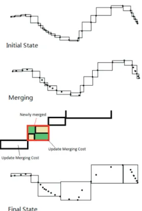
Stage 1: Trajectory segmentation. The segmentation process transforms a tra-jectory expressed by coordinate points into a sequence of MBRs. An illustrating process is depicted in Figure 10. In this process, smaller MBRs are aggregated into larger MBRs. Initially, each two consecutive points in a trajectory sequence resemble as diagonal vertexes of an MBR.
Figure 10: Main Steps of the Greedy Splitting Process
The next step is merging two direct adjacent MBRs. Since an MBR may have its left or right neighbour to merge, the criteria of merging is based on the merging
cost. Suppose two consecutive MBRsmbraand mbrb are merged to a new mbrab, the
merging cost is defined as [54] :
Cost(mbra, mbrb) =V ol(mbrab)−V ol(mbra)−V ol(mbrb)
Where Vol denotes the volume function of MBRs.
The merging that leads to a smaller volume is selected. In one round of the greedy splitting algorithm, this merging action repeats till all the MBRs are scanned.
The framework adopts a greedy-split algorithm [67] to balance the cost and ap-proximation quality. The implementation uses the data model defined. The full details of greedy-split are listed in Algorithm 7. The merging action is listed in Algorithm 8.
Algorithm 7 The Algorithm of Greedy Split
Input: T rp ={pt1, pt2,· · · }: a single spatio-temporal trajectory,
K: an integer denoting the final number of segments split into(All subscriptsT rp
are omitted compared to Table. 2)
Output: An MBR listM BRList={mbr1, mbr2,· · · } that covers T r
Creation of MBR :
1: for each South West Point ptSW ∈ T r and its consecutive right side
ptNE(assuming located at NE direction) do
2: create new Points
ptNW :=P oint(ptSW.x, ptNE.y), ptSE :=P oint(ptNE.x, ptSW.y)
3: create new MBR, with above four points as vertexes m :=
P olygon(ptSW, ptSE, ptNE, ptNW)
4: M BRList.insert(m)
5: end for
6: for eachtwo consecutive MBRsmbrl ∈M BRList and mbrr :=mbrl.next()do
7: call merging algorithm to mergembrlandmbrrto a new temporary MBRmbrlr
8: Cost(l, r) :=V olume(mbrlr)−V olume(mbrr)−V olume(mbrl)
9: CostQue.put(Cost(l, r)) 10: end for Merging loop : 11: while M.size()> k do 12: Cost(i, j) := CostQue.min() 13: mbri :=merge(mbri, mbrj) 14: M BRList.remove(mbrj), CostQue.remove(Cost(i, j))
15: merger mbri and mbrk :=mbri.next()
to get Cost(i, k)
16: CostQue.insert(Cost(i, k))
17: end while
Algorithm 8 The Algorithm of Merging MBRs
Input: one MBR mbra and its consecutive right side MBR mbrb
Output: a new MBR mbrabthat covers bothmbra and mbrb
1: Pa :=Pa∪Pb, wherePa and Pb is mbra and mbrb’s inside PointSet
2: get xmax :=M ax(Pa.X),
xmax :=M ax(Pa.Y) ,
xmin :=M in(Pa.X),
ymin :=M in(Pa.Y)
3: ptSW :=P oint(xmin, ymin) ,
ptSE :=P oint(xmax, ymin),
ptNE :=P oint(xmax, ymax),
ptNW :=P oint(xmin, ymax)
4: mbrab:=P olygon(ptSW, ptSE, ptNE, ptNW),
mbrabinside pointSet =Pa
5: return a new MBRmbrab covering mbra and mbrb
When data points are missing at certain timestamps, the algorithm uses the next available data point to merge MBRs. Therefore, in the implementation of the greedy split algorithm, the size of MBRs, as well as the time span of individual MBRs are both varied.
3.3.3
Parallel and Distributed Implementation
The greedy-split algorithm is independently applied to each trajectory. Thus the segmentation is processed in parallel. When the dataset contains a large number of trajectories that is beyond a single node’s capacity, the dataset can be partitioned on a cluster of nodes. Therefore, each partition contains a number of trajectories that are segmented in parallel.
To enable parallel processing on data partitioning, this study develops the greedy-split algorithm using Resilient Distributed Datasets (RDDs) in Apache Spark [72]. RDDs are first created by reading the dataset from stable storage such as HDFS into the partitioned collection of records. These RDDs are further transformed by
opera-tions such asmap, filter,groupBy,reduceand so on all elements in the dataset. So
nodes. Accordingly, different RDDs containing different data types correspond to objects defined in this data model. The transformations and operations on RDDs realize the greedy-split algorithm.
When the raw data are stored in HDFS or any other file system with distributed blocks like S3, the initial RDDs created by reading files from that are already dis-tributed and partitioned. The partition size and their distribution are inherited from HDFS’s block size and the partitions will be distributed into multiple nodes. At this time, the trajectories in the same partition origin from the same block in HDFS host. Each Geolife trajectory is a text-based file in the dataset. After reading to Spark,
each trajectory record is a <key, value> pair in the RDD. In each RDD record,
the key is the file name of that trajectory, and the value is the raw content of that file. Followed by that, the content is read line by line to create position records with
latitude, longitude and the timestamp to a Point in this data model.
After this transformation, it has a new <key,value>pair RDD, where the key is
still the file name and the value is this trajectory’s point list, asLinkedList<Point>.
The next transformation is using the greedy-split algorithm to group points into
MBRs described in this section. After this, the point list is replaced byMBRList. In
theMBRList, each MBR is a polygon element that contains the sub-trajectoryPoints
in its PointSet structure.
Afterwards, system uses the flatMaptransformation to flatten RDD’s value that
is represented as MBRList to a sequence of MBRs. The new RDD has the compound
key called MBRRDDKey that consists of two attributes. One attribute is the trajectory
name, and the other is trajectyr’s MBR sequence number in a chronological order
3.4
Partition and Indexing
The trajectory repartitioning shuffles all MBRs within a certain geographic bound-ary to the same partition. These spatio-temporal partitions form closures. Inside this closure, the framework can perform the intersection join operation. It further extends the spatial boundary with the temporal boundary, that means MBRs within a certain time period are also partitioned to the same node. Under this spatio-temporal repar-titioning, an intersection query to sub-trajectories occurs within the same partition.
This is different from the initial MBR based partition discussed in Section 3.3.3. In the initial MBR based partition, all MBRs of the same trajectory are located in the same partition, and all the trajectories with similar name prefix are also located in the same partition. Compared to the initial file based partition, the spatio-temporal partitioning significantly reduces the data shuffling in the following processing.
The workflow is depicted in Figure 11. This thesis notates activities of this data flow with numbers to present the techniques involved and the mapping of activi-ties in the distributed cluster deployment (depicted in Figure 12). Both workflows share stages. After segmentation, the in-memory processing framework stores MBRs in cluster node memories; and the graph database framework stores MBRs in the distributed graph database.
Query Trajectory Trajectory Data Sampling Trajectory MBR RDD Bulk Loading Spatial RDD MBR Spatial Join Query Spatial Join Result RDD Metric Calculation Final Metric Result Segmentation Indexing Duplication Elimination ❶ ❷ ❹ ❺ ❻ Shuffling ❼ Partition Grid ❹ ❸ ❷
(a) In-memory Processing Workflow
Query Trajectory Trajectory Data Sampling Trajectory MBR RDD Bulk Loading Graph Datastore MBR Spatial Join Query Spatial Join Result RDD Metric Calculation Final Metric Result Segmentation Inserting MBRs Duplication Elimination ❶ ❷ ❺ ❻ Create Layers ❼ Partition Grid ❸ ❷ Indexing ❸ ❹
(b) Graph Database Workflow
Spark Node 1 Spark Node 1
Spark Node 1
Spark Node 1 Spark Node 2Spark Node 2 Spark Node 3Spark Node 3 Spark Node 2
Spark Node 2 Spark Node 3Spark Node 3
Cloud Storage
Hadoop File APIs Hadoop File APIs Hadoop File APIs
Segmentation Segmentation Duplication Elimination Duplication Elimination Duplication Elimination Duplication Elimination Spark Node 1
Spark Node 1 Spark Node 2Spark Node 2 Spark Node 3Spark Node 3 Output Result Output Result Output Result Output Result Output Result Output Result Neo4j DB 1
Neo4j DB 1 Neo4j DB 2Neo4j DB 2 Neo4j DB 3Neo4j DB 3
Indexing
Indexing IndexingIndexing IndexingIndexing
Spatial Query Spatial Query Spatial Query Spatial Query Spatial Query Spatial Query GeoSpark Node 1
GeoSpark Node 1 GeoSpark Node 2GeoSpark Node 2 GeoSpark Node 3GeoSpark Node 3
Indexing
Indexing IndexingIndexing IndexingIndexing
Metric Calculation Metric Calculation Metric Calculation Metric Calculation Metric Calculation Metric Calculation Spatial Query Spatial Query Spatial Query Spatial Query Spatial Query Spatial Query Duplication Elimination Duplication Elimination Partitioning Partitioning ❺ ❻ ❼ ❶ ❷ ❸ ❸ B ❸ A ❹ Graph Datastore Workflow In-Memory Datastore Workflow Sampling&Bulk Loading Sampling&Bulk Loading Partitioning Partitioning Segmentation Segmentation Partitioning Partitioning Segmentation Segmentation Sampling&Bulk Loading Sampling&Bulk Loading Sampling&Bulk Loading Sampling&Bulk Loading
Figure 12: Dataflow Between Nodes
3.4.1
Partitioning Techniques
The Spatial Partition activity in the data flow uses a spatial partition method. The spatial partitioning methods include Equidistant, Hibert, Voronoi, Quad-tree and R-tree [16].
This study develops an R-tree partition to achieve balanced partition of MBRs. Since it aims to put MBRs within the same spatio-temporal boundary to the same partition. Therefore, the even distribution of MBRs among partitions is achieved
through the adjustment of boundary size. The boundary size of a partition is deter-mined by factors as the number of partitions and the number of trajectory MBRs. Assume there are 2000 MBRs after the segmentation process, and sample 1% MBRs to build the R-tree. Then it is 20 MBRs for building up boundaries for partitions. Assume further that the system can get 10 partitions, then boundary ranges are di-vided into the 10 ranges based on the 20 MBRs’s spatio-temprol span. In addition, there is one more range for any MBRs that are beyond the spatio-temporal range
from the samples called overflowed partition. In general, if it targets p number of
partition, it finally has p+ 1 ranges.
Each leaf node of the R-tree has even numbers of MBR objects contained. There-fore the boundary range of each leaf node is dynamically changed to make the bal-anced distribution of MBR objects. Since the range of each leaf node represents a geographic area within a period time, the adjustment of the range scale of a leaf node eventually modify the geographic area given a time covered by the partition, thus the density distribution of MBRs on each partition. If the objects in an area are scattered, this leaf node contains a larger range than average; if the objects in an area are dense, this leaf node contains a smaller range than average.
The thesis develops the R-tree spatial partition in-memory using GeoSpark. The major tasks and techniques are presented below.
Stage 2: Creating a geographical partitioning grid. In this step, the
framework creates a geological partitioning strategy. This is a spatial grid based on R-tree rectangles. There are two sub-steps including step 2.1 and 2.2.
Stage 2.1: Data sampling. The framework randomly samples 1% of the whole MBRs for establishing range boundaries of the partitions with R-tree. This sampling method avoids building a global index thus helps to reduce the computation cost.
Stage 2.2: Bulk loading. With the samples, the system builds the R-tree using the Sort-Tile-Recursive (STR) algorithm [27] to split overflowed nodes. The STR
algorithm estimates the number of leaves required as l =samplesize/p, except the
last overflowed partition that represents the rest of range of boundaries outside the
boundaries of samples. Eventually, the R-tree has l+ 1 leaves. Each leaf represents
one geological boundary. The generated R-tree is stored as aSpatialRDD for further
query usage. SpatialRDD is an abstract class that stores geometry distributively
Distance Join, Range Query, KNN Query or even saving as text files.
Stage 3: Data shuffling or migration. In this step, there are several sub-steps marked as 3.1, 3.2 and 3.3.
Stage 3.1: Partition assignment. When an MBR imported has an intersection with any leaf node boundary in the R-tree, the MBR is assigned to the partition number that the leaf node belongs to. The partition ID number becomes the key
to the MBR’s RDD. A replication method is further developed to handle the cases
that boundaries may have overlapping or one MBR is large enough to across multiple
partitions. With this replication method, the MBR across multiple boundaries of
partitions is assigned to multiple partitions. To make the query result consistent, duplicated copies are removed after a query. The assignment algorithm is shown in Algorithm 9.
Algorithm 9 Algorithm for R-tree Partition Assignment
Input: mbrT rc: one trajectoryT rc segmented Candidate MBR and
partitionList: the partition grid generated from R-tree partition method
Output: a partition ID indicating which partition it belongs to
1: containFlag := false
Iterate Each Partition :
2: for each ith partition from partitionList do
3: if partitioni covers mbrT rc then
4: partitionID := i
/*Contain only check*/
5: containFlag := true
6: else if P artitioni intersectsmbrT rc then
7: partitionID := i
8: end if
9: end for
10: if containFlag is false then
11: partitionID = overflow
12: end if
13: return partitionID
3.4.2
Data Shuffling
All MBRs within the same geographical partition should be located on the same
Spark worker node. This redistribution process involvesshuffling RDDs in GeoSpark
In the following steps, the thesis uses A suffix to distinguish the stages occurring
in the in-memory framework and use B suffix to express the stages occurring in the
graph storage framework.
Stage 3.2A: Repartition. The framework applies thepartitionBy() function in Spark to locate all MBRs (in RDDs) with the same key to the same partition. This incurs data shuffling between Spark nodes.
3.4.3
Data Persistence
The persistent method of MBRs migrates the MBRs in Spark RDDs to the NoSQL database, Neo4j. To support the spatial data model, the framework deploys the Neo4j-spatial extension [64] that contains map layers. A Neo4j
![Figure 3: Modelling Object Interactions. [7]](https://thumb-us.123doks.com/thumbv2/123dok_us/533193.2562873/19.918.218.759.123.649/figure-modelling-object-interactions.webp)
![Figure 4: An R-tree Structure [2]](https://thumb-us.123doks.com/thumbv2/123dok_us/533193.2562873/23.918.249.726.113.698/figure-an-r-tree-structure.webp)
![Figure 5: SQL Server Indexing [1]](https://thumb-us.123doks.com/thumbv2/123dok_us/533193.2562873/26.918.216.759.124.623/figure-sql-server-indexing.webp)
![Figure 6: Overview of YARN Architecture [34]](https://thumb-us.123doks.com/thumbv2/123dok_us/533193.2562873/30.918.155.816.422.735/figure-overview-of-yarn-architecture.webp)
![Figure 8: The Trajectory MBR in 3-D. [9]](https://thumb-us.123doks.com/thumbv2/123dok_us/533193.2562873/36.918.323.647.125.423/figure-the-trajectory-mbr-in-d.webp)