Dissertations
Spring 5-2011
Microarray Data Mining and Gene Regulatory Network Analysis
Microarray Data Mining and Gene Regulatory Network Analysis
Ying Li
University of Southern Mississippi
Follow this and additional works at: https://aquila.usm.edu/dissertations
Part of the Computational Biology Commons
Recommended Citation Recommended Citation
Li, Ying, "Microarray Data Mining and Gene Regulatory Network Analysis" (2011). Dissertations. 477.
https://aquila.usm.edu/dissertations/477
This Dissertation is brought to you for free and open access by The Aquila Digital Community. It has been accepted for inclusion in Dissertations by an authorized administrator of The Aquila Digital Community. For more
MICROARRAY DATA MINING AND GENE REGULATORY NETWORK ANALYSIS
by Ying Li A Dissertation
Submitted to the Graduate School of The University of Southern Mississippi in Partial Fulfillment of the Requirements for the Degree of Doctor of Philosophy
MICROARRAY DATA MINING AND GENE REGULATORY NETWORK ANALYSIS
by Ying Li May 2011
The novel molecular biological technology, microarray, makes it feasible to obtain quantitative measurements of expression of thousands of genes present in a biological sample simultaneously. Genome-wide expression data generated from this technology are promising to uncover the implicit, previously unknown biological knowledge. In this study, several problems about microarray data mining techniques were investigated, including feature(gene) selection, classifier genes identification, generation of reference genetic interaction network for non-model organisms and gene regulatory network reconstruction using time-series gene expression data. The limitations of most of the existing computational models employed to infer gene regulatory network lie in that they either suffer from low accuracy or computational complexity. To overcome such
limitations, the following strategies were proposed to integrate bioinformatics data mining techniques with existing GRN inference algorithms, which enables the discovery of novel biological knowledge. An integrated statistical and machine learning (ISML) pipeline was developed for feature selection and classifier genes identification to solve the challenges of the curse of dimensionality problem as well as the huge search space. Using the selected classifier genes as seeds, a scale-up technique is applied to search through major databases of genetic interaction networks, metabolic pathways, etc.
against well-studied genetic model organisms, a reference gene regulatory network for less-studied organisms was built and used both as prior knowledge and model validation for GRN reconstructions. Networks of gene interactions were inferred using a Dynamic Bayesian Network (DBN) approach and were analyzed for elucidating the dynamics caused by perturbations. Our proposed pipelines were applied to investigate molecular mechanisms for chemical-induced reversible neurotoxicity.
YING LI 2011
MICROARRAY DATA MINING AND GENE REGULATORY NETWORK ANALYSIS
by Ying Li A Dissertation
Submitted to the Graduate School of The University of Southern Mississippi in Partial Fulfillment of the Requirements for the Degree of Doctor of Philosophy
Approved: Chaoyang Zhang Director ____ Nan Wang______________________ ____ Ping Gong______________________ Edward J Perkins Andrew Strelzoff
Dean of the Graduate School Susan A Siltanen
I would like to thank Dr. Nan Wang, Dr. Chaoyang Zhang, and all the other
committee members, Dr. Ping Gong, Dr. Edward J. Perkins, and Dr. Andrew Strelzoff, for their suggestions and advice to improve my work during the whole process. I
gratefully acknowledge my advisors, Dr. Wang and Dr. Zhang, for their generous help in the past four years. Along the path of research that has led to this dissertation, they have constantly been there to provide me guidance, support and suggestions. I also would like to thank Dr. Ping Gong and Dr. Edward Perkins for their comments and for providing high-quality data during my doctoral research.
I am forever indebted to my parents, who have been extremely supportive and helpful despite living thousands miles away. My father always encourages me to do what I want to do, and my mother believes I am the best in the world, which gives me a lot of
confidence. I am especially thankful to all other collaborators in Engineer Research and Development Center Environmental Lab in Vicksburg, MS. They gave me a lot of help when I was working there during my Ph.D. program.
ABSTRACT ... ii
ACKNOWLEDGMENTS ... iv
LIST OF TABLES... vii
LIST OF ILLUSTRATIONS... ix
CHAPTER I. INTRODUCTION ...1
Biological Background DNA Microarray Technology Microarray Data Analysis Contributions Dissertation Organization II. REVIEW OF MICROARRAY DATA MINING ...13
Microarray Experiments and Data Generation Microarray Data Preprocessing Identification of Differentially Expressed Genes (DEGs) Feature Selection Inference of Gene Regulatory Networks (GRNs) III. IDENTIFY CLASSIFIER GENES USING ISML PIPELINE...26
Integrated Statistical and Machine Learning (ISML) Pipeline Feature Filtering by Statistical Analysis Classifier Gene Selection and Ranking Optimization by Machine Learning Approaches Identification of Significant Pathways IV. REFNET: A TOOLBOX TO RETRIEVE REFERENCE NETWORK...37
Basic Local Alignment Search Tool (BLAST) KEGG Metabolic Pathways and GRN Database
RefNet: Reference Network for Non-Model Organisms Interpretation of Retrieved Reference Network
Information Theory
Boolean Network and Probabilistic Boolean Network (PBN) Bayesian Network and Dynamic Bayesian Network (DBN) Learning Bayesian Network
Time-Delayed Dynamic Bayesian Network
VI. MICROARRAY DATA MINING: CASE STUDY...65 Multi-Class Earthworm Microarray Dataset
Identification and Optimization of Classifier Genes Time-Series Earthworm Microarray Dataset
Identification and Optimization of Classifier Genes
Reconstruction of GRNs for Chemical-Induced Neurotoxicity
VII. CONCLUSIONS ...118 Summary and Conclusions
Future Directions
REFERENCES ...121
Table
3.1. Tree-Based Classifier Algorithms in WEKA...32
4.1. Different BLAST Programs………...42
4.2. Commonly Used Public Databases of Genetic Interactions….……….……44
4.3. KEGG Databases………..……….45
5.1. Methods for Learning Bayesian Network Structure and Parameter Determination………....62
6.1. Summary of Classification Results Using Tree-Based Classification Algorithms……….75
6.2. Confusion Matrix Showing Classification Results Using 39 Classifier Genes by SVM………...……..…..78
6.3. Confusion Matrix Showing Classification Results Using 30 Classifier Genes by Clustering………...…...….78
6.4. Confusion Matrix Showing Classification Results Using 58 Classifier Genes by SVM or Clustering………...………..80
6.5. Optimized Set of 58 Classifier Genes………...…….81
6.6. Summary of Classification Results Using Tree-Based Classification Algorithms……….93
6.7. Confusion Matrix Showing Classification Results Using 45 Classifier Genes by SVM.……….……….96
6.8. Confusion Matrix Showing Classification Results Using 49 Classifier Genes by Clustering..………...98
6.9. Confusion Matrix Showing Classification Results Using 70 Classifier Genes by SVM or Clustering…………..………...99
6.10. Summary of Nine Identified Significant Pathways……….101
6.11. Summary of Inferred GRNs for MAPK Pathway by DBN Model…………..…109 vii
6.13. Summary of Inferred GRNs for Huntington’s Disease Pathway by DBN
Model………...………113 6.14. Summary of Comparing Inferred GRNs in Three Treatment Conditions……...117
Figure
1.1. Central Dogma of Molecular Biology……..………...2
1.2. Transcription and Translation Process………...………...4
1.3. Regulations of Genes………...………....5
1.4. Workflow of Microarray Experiment………..7
2.1. Process of cDNA Microarray Experiment Design……….14
2.2. Intensity Distribution of Arrays Before and After Median Normalization……....18
2.3. Spot Intensity Plots with Different Lowess Window Width………...19
2.4. Comparison of KNN, SVD, and Row Average Based Estimations’ Performance on the Same Data Set …...20
2.5. Intensity-Dependent Z-Scores for Identifying Differential Expression………….21
2.6. Key References for Feature Selection Technique in Microarray Domain...23
2.7. A Typical Gene Regulatory Network...25
3.1. Overview of the ISML Pipeline...28
3.2. Classifier Tree Models with Corresponding Accuracy…………...……..……….33
4.1. Overview of the RefNet Analysis Platform...39
4.2. Overall Procedure of RefNet...46
5.1. Relationship between Entropy and Mutual Information………..…………..50
5.2. An Example of Boolean Network……….……….53
5.3. A Basic Building Block of a PBN……….………54
5.4. A Simple Example of Bayesian Network……….….57
5.5. Static Bayesian Network and DBN………...……….58 ix
5.7. Process of Time Lag DBN………64
6.1. Summary of DEGs in Multi-Class Earthworm Microarray Dataset.……….71
6.2. Screenshots of Gene Expression Data of Multi-Class Earthworm Dataset...72
6.3. Application of ISML Pipeline in Multi-Class Earthworm Dataset…...73
6.4. The Accumulative Distribution (a) and Histogram (b) of Weights of 354 Classifier Genes………...………..75
6.5. Classification Accuracy Using 354 Classifier Genes by SVM or Clustering...76
6.6. Classification Accuracy Using 39 or 30 Classifier Genes by SVM or Clustering, Respectively……….………...77
6.7. Array Distribution of Three Treatments and 31 Time Points...89
6.8. Sampling Scheme of 44K Time-Series Earthworm Microarray Dataset...90
6.9. Application of ISML Pipeline in Time-Series Earthworm Dataset...91
6.10. The Accumulative Distribution (a) and Histogram (b) of Weights of 1074 Classifier Genes...94
6.11. Classification Accuracy Using 1074 Classifier Genes by SVM or Clustering...95
6.12. Classification Accuracy Using 45 or 49 Classifier Genes by SVM or Clustering, Respectively...97
6.13. Reference Pathway for Alzheimer’s Disease Built by RefNet……….…...100
6.14. Reference Pathways of (a) MAPK and (b) Huntington’s Disease built by RefNet………...102
6.15. A Curated Reference Network of 38 Genes from MAPK Pathway………104
6.16. List of 38 Genes from MAPK Pathway for Reconstruction of GRN …………..105
6.17. Inferred GRNs of 38 Genes from MAPK Pathway……….…106
6.18. Summary of common edges between Six Inferred GRNs with Curated Reference Network, Respectively………...……….…109
6.20. Inferred GRNs of 40 Genes from Huntington’s Disease Pathway…………..…114
CHAPTER I INTRODUCTION Biological Background
Central Dogma of Molecular Biology
The Central Dogma of genetics [1] is: DNA is transcribed to RNA which is translated to protein. Protein is never back-translated to RNA or DNA, and DNA is never directly translated to protein. This dogma forms the backbone of molecular biology and is represented by four major stages: (1) replication: the DNA replicates its information in a process that involves many enzymes; (2) transcription: the DNA codes for the production of messenger RNA (mRNA); (3) In eukaryotic cells, the mRNA is processed (essentially by splicing) and migrates from the nucleus to the cytoplasm; (4) translation: messenger RNA carries coded information to ribosome. The ribosome “read” this information and uses it for protein synthesis. Proteins do not code for the production of protein, RNA or DNA. They are involved in almost all biological activities, structural or enzymatic. We often concentrate on protein coding genes, because proteins are the building blocks of cells and the majority of bio-active molecules. Figure 1.1 shows the central dogma of molecular biology [1].
The relationships of DNA, RNA, and Proteins are: Proteins determines the activity of the cells. They are the physical format of the abstract information integrated in the genome. DNA contains the genetic information and each cell has a copy. It is stable, packaged, and inert. RNA is the messenger and translator. It is unstable and lacks secondary structure. Some RNA has enzymatic activity.
Figure 1.1.Central dogma of molecular biology [1]. Genes and Proteins
Genes are made of millions of deoxyribonucleic acid (DNA) molecules. A DNA molecule is constructed like a spiral staircase, or a double helix. The rails of the staircase are made of a backbone structure of phosphates and sugars, and the steps are pairs of four nitrogen-containing bases: adenine (A), cytosine (C), guanine (G), and thymine (T). Through hydrogen bonds the two rails of the staircase are kept together, A and T pair together, and C and G are partners [2].
A gene is made of a unique sequence of DNA bases. It is like a message containing a unique combination of letters. Then a translation of this message into information for protein production is performed. A protein is a folding chain of amino acids following a specific order. Altogether there are 20 different amino acids exist. The message for each amino acid within a protein is coded by a combination of three nucleotide bases. If the sequence in the message is misspelled, it will have a point mutation. As a result, the gene may produce a protein that has an incorrect shape so it won't combine with another protein (e.g., a receptor), leading to a mistake in the resulting message due to the unfitting
shape. In other words, if the message in the gene is misspelled, the protein it encodes may be wrong and its function in the body may be changed. In general, experimental and computational evidence shows that many genes produce an average of three different proteins and as many as ten protein products. The protein-coding regions of a gene are called exons, while the non-coding regions are called introns. Due to alternative splicing, the exons of a gene can be combined in different ways to make variants of the complete protein [3].
Gene Expression
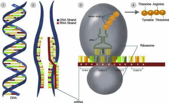
By using the information from the DNA sequence of a gene, the synthesis of functional gene products is usually called gene expression. In Figure 1.2, it shows that there are two major steps in gene expression: transcription of DNA and translation of mRNA
into protein. Here, the products are often proteins or functional RNA. Protein is
considered the most basic building block of life. The roles that proteins play in the process of life include constituting cell structures, regulating cellular processes,
catalyzing biochemical reactions in metabolic pathways, etc. The specific functions of a certain protein are determined by its particular physical structure and chemical properties.
Several steps in the gene expression process may be modulated, including the
transcription, RNA splicing, translation, and post-translational modification of a protein. Gene regulation gives the cell control over structure and function, and is the basis for cellular differentiation, morphogenesis and the versatility and adaptability of any organism. Gene regulation may also serve as a substrate for evolutionary change, since control of the timing, location, and amount of gene expression can have a profound effect on the functions of the gene in a cell or in a multicellular organism.
Figure 1.2.Transcription and translation process. Source from
http://publications.nigms.nih.gov/thenewgenetics/chapter1.html
Gene Regulation
Gene regulation is the processes of cells regulate the information in genes to be turned into gene products. The majority of known mechanisms regulate protein coding genes although the product of a functional gene may be RNA or protein. A gene’s expression could be modulated at any step, for instance, DNA-RNA transcription, or
post-translational modification of a protein, etc. The regulation of gene’s expression plays vial roles due to its increase of the versatility and adaptability of an organism by allowing the cell to express proteins when needed. Besides, the processes of cellular differentiation and morphogenesis are driven by gene regulation. Such processes lead to the creation of different cell types in multicellular organisms.
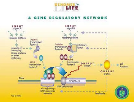
A gene regulation system consists of genes, cis-elements, and regulators [3]. The regulatory process of genes is illustrated in Figure 1.3. The regulators in the system could
be proteins in most cases, but small molecules such as miRNAs and metabolites may also be regulators sometimes. Such proteins that participate in the process of regulation are called transcription factors (TFs), or they are also referred to as trans-elements. The cis-elements, which are the complementary to trans-cis-elements, are DNA segments that control the expression of corresponding genes.
Figure 1.3.Regulations of genes.
There are six stages where gene expression is regulated: chromatin, domains, transcription, post-transcriptional modification, RNA transport, translation, and mRNA degradation. Any step of gene expression could be modulated. Among these stages, the most extensively utilized point is transcription initiation. There two major cases of regulation of gene expression, namely up-regulation and down-regulation. Up-regulation
occurs within a cell, which results in increased expression of one or more genes while down-regulation results in decreased gene expression and corresponding protein
expression. The regulation mechanism includes the binding of certain TFs to cis-elements and then controls the level of target gene’s expression during transcription. A gene’s expression is regulated by some regulators, while its own expressed products can be regulators of another gene. The gene regulatory network (GRN) is formed by such complex regulatory connections [3].
DNA Microarray Technology
Functional genomics involves the analysis of large datasets of information derived from various biological experiments. One such type of large-scale experiment involves monitoring the expression levels of thousands genes simultaneously under a particular condition, called gene expression analysis. Microarray technology makes use of the sequence resources created by the genome projects and other sequencing efforts to answer the question, what genes are expressed in a particular cell type of an organism, at a particular time, under particular conditions.
DNA Microarray
A DNA microarray is a multiplex technology used in molecular biology, which consists of an arrayed series of thousands of microscopic spots of DNA oligonucleotides, called features (genes). Each feature contains picomoles (10-12moles) of a certain DNA sequence, which are also known as probes. Such probes can be a fragment of a gene or other DNA element which are used to hybridize with a cDNA/cRNA sample under experimental designed conditions. A microarray experiment is able to accomplish several genetic tests in parallel because tens of thousands of probes can be included in an array. Thus, microarray technology allows us to monitor tens of thousands of gene expressions
and have significantly accelerated the investigations of many types of biology experiments. Figure 1.4 illustrated the overall workflow of a microarray experiment.
Figure 1.4.Workflow of microarray experiment. Source from
http://images-mediawiki-sites.thefullwiki.org/06/3/9/3/8878261581107656.png
Microarray technology evolved from Southern blotting, where fragmented DNA is attached to a substrate and then probed with a known gene or fragment. The use of a collection of distinct DNAs in arrays for expression profiling was first described in 1987, and the arrayed DNAs were used to identify genes whose expression is modulated by interferon [4]. These early gene arrays were made by spotting cDNAs onto filter paper with a pin-spotting device. The use of miniaturized microarrays for gene expression profiling was first reported in 1995 [5], and a complete eukaryotic genome on a microarray was published in 1997 [6].
Microarray Types and Applications
There exist many types of microarrays and they are differed by whether being
spatially arranged on a surface or on coded beads. The early-stage array is a collection of orderly microscopic spots. Each spot is combined with a specific probe attached to a solid surface, such as silicon, glass or plastic biochip. The location of a certain probe has been arranged and thousands of these probes are placed on a single DNA microarray. On the alternative, bead array is a collection of microscopic polystyrene beads. A specific probe
and a ratio of two or more dyes are combined with each bead. Thus, they do not interfere with the fluorescent dyes used on the target sequence. DNA microarrays technology can be used in many areas such as gene expression profiling, comparative genomic
hybridization, chromatin immunoprecipitation on Chip (ChIP), SNP detection, alternative splicing detection [4, 5, 7, 8] and etc.
Microarray Data Analysis
Microarray experiments are inexpensive compare to many other biological experimental technologies. However, there exist several specific bioinformatics challenges as follows: first one is the multiple levels of replication in experimental design. Due to the biological complexity of gene expression, experiment design of a microarray experiment is critically important if statistically and biologically valid conclusions need to be elucidated from the data [9]. The second challenge is the number of platforms and distinct groups and data format. Microarray data is impossible to be exchanged due to the lack of standard protocols in platform fabrication, assay types, and analysis approaches. The "MicroArray Quality Control (MAQC) Project" is being
conducted by the US Food and Drug Administration (FDA) to form standards and quality control metrics which will allow the use of microarray data in many fields such as drug discovery, clinical practice and regulatory decision-making [10, 11]. The third challenge is statistical analysis regards to accuracy and precision. Microarray data sets are normally of huge amount, and its analytical precision is influenced by several variables. Statistical challenges include effects of image background noise, whether appropriate normalization and transformation techniques are conducted, identification of significantly differentially expressed genes (DEGs) [12, 13, 14, 15] as well as inference of gene regulatory networks
[16]. How to reduce the dimensionality of microarray dataset in order to obtain more comprehension and focused analysis requires further preprocess of microarray data [17].
Contributions
In this dissertation, we have made a number of contributions in identification and optimization of classifier genes and significant pathways. Based on such information, reconstruction of gene regulatory networks of interested pathways was performed, and all above work were summarized below.
Identification and Optimization of Classifier Genes
One important goal of microarray experiments is to discover novel classifier genes which play vital roles in genetic and molecular interactions. Microarrays have been successfully served as a research tool in discovering novel drug targets [18] and disease-or toxicity-related biomarker genes fdisease-or cancer classification [19]. A challenge in
classifying or predicting the diagnostic categories using microarray data is the curse of dimensionality problem coupled with sparse sampling. That is, the number of examined genes per sample is much greater than the number of samples that are involved in classification [20]. The other crucial challenge is that the huge search space for an optimal combination of classifier genes renders high computational expenses [21]. To address these two issues, we developed the new Integrated statistical and machine learning (ISML) pipeline, which integrates statistical analysis with supervised and unsupervised machine learning techniques. A set of classifier/biomarker genes from high dimensional datasets were identified and classification models of acceptable precision for multiple classes were generated as well by our pipeline. More details will be discussed in Chapter III.
Reference Network Builder
Gene Regulatory Networks (GRNs) provide integrated views of gene interactions that control biological processes. Many public databases contain biological interactions extracted from literature with experimental validations, but most of them only provide information for a few genetic model organisms. A number of computational models have been developed to infer GRN from microarray data, and these models are often evaluated on model organisms. Researchers who work with non-model organisms rely on these computational models to build GRN for less-studied organisms. However, they can only evaluate GRNs built by computational models based on the evaluation criteria such as recall, precision tested on model organisms. The accuracy and reliability of the tools are critical for non-model organisms. The researchers also are interested in evaluating the GRN based on “true” GRN of their organisms. Although, some public network databases provide experimentally validated interactions among genes or proteins, there are
limitations in accessibility and scalability. Thus, we developed a cyber-based integrated environment, called "reference network (RefNet)", to build a reference gene regulatory network for less-studied organisms. The resulting reference network could be used for validation of inferred GRNs or as prior knowledge for further inference.
Gene Regulatory Network Reconstruction
In the past, many computational models have been proposed to infer gene regulatory networks. Among them Probabilistic Boolean Network (PBN) [22, 23, 24, 25, 26] and Dynamic Bayesian Network (DBN) [27, 28, 29, 30, 31] are two popular and powerful models. PBN is a discrete state space model which characterizes a system using quantized data, while DBN is an extension of Bayesian network model to incorporate temporal concept. Previous studies showed that both PBN and DBN approaches had good
performance in modeling the gene regulatory network, but DBN identified more gene interactions and gave better accuracy than PBN [32]. Besides, Zou et al.[28] used DBNs
with various time-delays, by shifting time-series profiles with properly predicted amount of time steps. Therefore, we used the time-lagged DBN to reconstruct those chemical-induced networks/pathways which were identified by the RefNet (see Chapter IV) to analyze the dynamics caused by perturbations.
Dissertation Organization
This dissertation is organized as follows: In Chapter II, we introduce some basic concepts and backgrounds of microarray experiments and gene regulatory networks. Then some data preprocessing methods and techniques based on microarray data are introduced, such as transformation, normalization, etc. We also discuss some statistical models to identify differentially expressed genes such as t-test, ANOVA and others for either two-class comparison or multi-class comparison. Then, some machine learning methods such as clustering, classification based on microarray data for feature selection and identification of biomarker genes are reviewed.
In Chapter III, we proposed an integrated pipeline combining statistical analysis and machine learning approaches to identify a set of classifier genes for disease diagnostic and toxicity evaluation. We assembled an integrated statistical and machine learning pipeline consisting of several well-established feature filtering/selection and classification techniques to analyze microarray dataset in order to construct classifier models that can separate samples into different treatment groups such as evaluating toxicity exposure in certain environment or diagnosing cancer patients from normal people, etc.
In Chapter IV, a cyber-based environment to retrieve reference genetic interaction network (RefNet) is proposed. Our RefNet toolbox provides the following services: (1) to
build reference GRN/Pathway for non-model organisms; (2) to provide biological prior knowledge of GRN to improve computational models; (3) to interpret and compare the GRNs built from computational models with wet-lab experiments; and (4) to serve as a gene selection tool for GRN reconstruction.
In Chapter V, we introduced and discussed various computational methodologies to infer gene regulatory network. A review of existing inferring algorithms such as Boolean networks, Bayesian networks, and Dynamic Bayesian network is given. The time-lagged dynamic Bayesian network model was used to reconstruct sets of genes from selected pathways by RefNet. Results showed that our strategy helped with the improvement of accuracy as well as computational cost of GRN reconstruction and novel biological knowledge was discovered. In Chapter VI, by integrating all the toolkits and services for microarray data mining and gene regulatory network analysis, we presented two case studies to present the detailed contextual analysis.
We complete the dissertation by summarizing our work, and providing sets of issues appropriate for future work in Chapter VII.
CHAPTER II
REVIEW OF MICROARRAY DATA MINING Microarray Experiments and Data Generation
A microarray experiment requires a number of cDNA or oligonucleotide DNA sequences (probes) that are affiliated to a glass, nylon, or quartz wafer (adopted from the semiconductor industry and used by Affymetrix, Inc. [33]). Then material containing RNA, which is acquired from the biological samples to be studied, is mixed with this array. For example, the mixture of samples from normal tissues with samples from cancer tissues. Figure 2.1 illustrates the basic process of cDNA microarray experiments.
Microarrays can be manufactured using various technologies. In spotted microarrays, the probes are oligonucleotides, cDNA or small fragments of PCR products that
correspond to mRNAs. The probes are synthesized prior to deposition on the array surface and are then "spotted" onto glass. The resulting grid of probes represents the nucleic acid profiles of the prepared samples. This provides a relatively low-cost
microarray that may be customized for each study, and avoids the costs of interest to the investigator. However, publications exist which indicate such microarrays may not
provide the same level of sensitivity compared to commercial oligonucleotide arrays [34]. In oligonucleotide microarrays, the probes are short sequences designed to match parts of the sequence of known or predicted Expressed Sequence Tags (ESTs), which is a short sub-sequence of a transcribed cDNA sequence [35]. Oligonucleotide arrays are produced by printing short oligonucleotide sequences designed to represent a single gene or family of gene splice-variants by synthesizing this sequence directly onto the array surface instead of depositing intact sequences. Sequences may be longer (60-mer probes such as the Agilent design) or shorter (25-mer probes produced by Affymetrix) depending on the
desired purpose; longer probes are more specific to individual target genes, shorter probes may be spotted in higher density across the array [36].
Figure 2.1.Process of cDNA microarray experiment design. Source from
http://www.microarray.lu/en/MICROARRAY_Overview.shtml
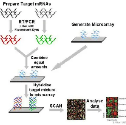
Two-color microarrays or two-channel microarrays are typically hybridized with cDNA prepared from two types of samples to be compared (i.e., chemical-treated sample versus un-treated sample) and they are labeled with two different fluorophores [37]. Cy3
and Cy5are two common fluorescent dyes that are used for cDNA labeling. The two
Cy-labeled cDNA samples are mixed and hybridized to a single microarray which is then scanned in a microarray scanner to measure the intensities of fluorescence of the two fluorophores after excitation with a laser beam of a defined wavelength. Relative
intensities of each fluorophore are then used to identify up-regulated and down-regulated genes [38]. In single-channel or one-color microarrays, the array provides intensity data for each probe indicating a relative level of hybridization with the labeled target.
However, this intensity data is not true indicator of abundance level of a gene, but rather a relative abundance when compared with other samples processed in the same
experiment. Since each chip is exposed to only one sample as opposed to two-channel platform, the single-channel system is more accurate. In one-color array chip, an aberrant sample cannot affect the raw data derived from other samples. While in two-color array chip, a single low-quality sample may drastically impinge on the precision of overall data set even if the other sample was of high quality. Another advantage of single-channel chip is that it is much easier when comparing data to arrays from different experiments as long as batch effects are taken care of.
Microarray Data Preprocessing
Image Processing Analysis
The population of mRNA in a certain sample can be stored as an image with intensity values indicating the relative expression level for each gene. The array chips are scanned by microarray scanners, which are provided by microarray manufacturers, and the intensity values of each spot on the chip are recorded. Image processing involves the following steps: (1) Identification of the spots and distinguishing them from spurious signals. The microarray is scanned following hybridization and an image file is
generated. Once image generation is completed, the image is then analyzed to identify spots and used to identify regions that correspond to spots; (2) Determination of the spot area will be studied and identification of the local region is used to estimate background noise. After identifying regions that correspond to sub-arrays, in order to get a
measurement of the spot signal and estimated for background intensity, a region within the sub-array needs to be selected; (3) Reporting statistics summary and generate spot intensity by subtracting background intensity. In this step, once the center and
background areas have been determined, a number of statistics summary for each spot are reported. Another concern in image processing is the number of pixels to be included for measurement in the spot image [39@)RUPDQ\VFDQQHUVWKHGHIDXOWSL[HOVL]HLVȝP
However, it is better to use a smaller pixel size to make sure enough pixels included. Even though using a smaller pixel size increases the confidence in the measurement, the image size tends to be bigger when compared with ones using larger pixel size.
Data Normalization and Transformation
The purpose of normalization is to eliminate variations to allow appropriate comparison of data that is obtained from each sample. Comparison of different arrays/samples normally involves making adjustments for systematic errors which is introduced by different procedures and effects. The order of operations for filtering the data is that spot filters are applied first, then data normalization, and then truncation of extreme values, then gene screening.
Spot filtering refers to filters on spots in individual arrays. Spot filtering is used for quality control purposes, i.e., to filter out “bad” spots. Unlike gene screening, Spot filtering does not filter out the entire gene (a row), but replaces the existing values of a spot within any given array with a missing value. There exist four types of spot filters: intensity filter, spot flag filter, spot size filter and detection call filter. The intensity filter is applied to the background adjustment of signals and different parameters are adopted for dual-channel or single-channel data. The spot flag filter can contain both numeric and character values. Outside of a specified numeric range, a flag is considered to be
“excluded”. For example, in Affymetrix array, a Detection Call column is used to designate as the spot flag at the time of collating, which allows the users to filter out expression values that have an “A” (Absent) call. Additionally, the spot flag is also used
to filter out spots with a large percentage of expression values that have a spot flag value of “A”.
In general, a logarithmic (base 2) transformation is applied to the signal intensities (for single-channel data) or intensity-ratios (for dual-channel data) before they are normalized and truncated. There are currently four major normalization options: median
normalization, housekeeping gene normalization, lowess normalization as well as print-tip group normalization. The first two are available for both single-channel and dual-channel data, but the last two are only for dual-dual-channel data. For single-dual-channel data, the user needs to choose a reference array against which all other arrays will be normalized. The “median” reference array is selected as following algorithm:
(1) Let N be the number of experiments, and let ibe an index of experiments running
from 1to N.
(2) For each array i, the median log-intensity of the array (denoted Mi) will be
computed.
(3) A median Mwill be selected from the {M1,…,MN}values. If N is even, then the median Mwill be the lower of the two middle values.
(4) The array whose median log-intensity Miequals the overall median Mwill be chosen as the median array.
Then, the median normalization is performed by subtracting out the median log-ration for each array, so that each normalized array has a median log-ration of 0. Such median normalization is called per-gene normalization. Besides, per chip normalization is
performed by computing a gene-by-gene difference between each array and the reference array, and subtracting the median difference from the log-intensities on that array, so that the gene-by-gene difference between the normalized array and the reference array is 0.
Figure 2.2.Intensity distribution of arrays before and after median normalization.
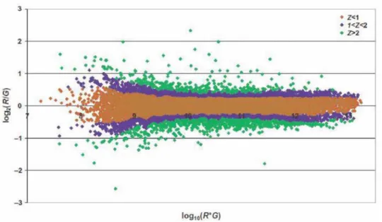
For dual-channel data, locally weighted linear regression (LOWESS) normalization is normally used. In the lowess normalization, a non-linear lowess smoother function is fit to the graph of un-normalized log-ratio on the y-axis versus average log intensity (i.e.,
[log(R)+log(G)]/2) on the x-axis. That is, lowess normalization assumes that the dye bias
appears to be dependent on spot intensity. The adjusted ratio is computed by the following Equation 2.1:
logܴ
ܩ ՜log
ܴ
ܩെ ܿ(ܣ) (2.1)
where c(A)is the lowess fit to the logܴ/ܩ versus logξܴమ ×ܩ plot. Lowess regression is
a technique for fitting a smoothing curve to a dataset. The degree of smoothing is
determined by the window width parameter. In general, a larger window width results in a smoother curve, while a smaller window results in local variation [40, 41, 42, 43]. Figure 2.3 shows the plots under different lowess window width.
Figure 2.3.Spot intensity plots with different lowess window width. Missing Values
After applying various techniques of normalization or filtering, missing expression values may exists in the data sets. However, many further gene expression analysis require a complete matrix of array values. Even missing values are allowed for some analysis algorithms, they are treated as intensity value of zero when calculated, which will certainly affect the accuracy and validity of analysis results. Therefore, methods for imputing missing data are needed to minimize the effect of incomplete data sets.
Previously, three most popular methods to impute missing values are proposed, namely, Singular Value Decomposition (SVD) based method (SVDimpute) [45, 46, 47], weighted
K-nearest neighbors (KNNimpute) [44], as well as row average. The KNN-based method
selects genes whose expression profiles are similar to the gene of interest to impute missing values. Suppose there is a missing value in experiment 1 for gene A, KNNimpute will find Kother genes whose expression values are most similar to A in experiments 2to N. Euclidean distance, which is the metric for gene similarity is used during the imputing
containing missing values and filling them with it. SVDimpute method can only be performed on complete matrices, so row average is imputed for all missing values and then utilize an expectation maximization method to arrive at the final estimate.
Troyanskaya et al.compared the above three missing value imputation techniques and
KNN-based estimations turned out to have best performance among the three on the same data set.
Figure 2.4.Comparison of KNN, SVD, and row average based estimations’ performance
on the same data set [44].
Identification of Differentially Expressed Genes (DEGs)
One of the common interests of microarray analysis is to identify genes that are significantly differentially expressed. Such DEGs are ones with expression ratio significantly different from 1 and are considered as important genes in later analysis study such as classification, clustering, or gene regulatory network reconstruction. Although some clustering techniques are used to find groups of genes with similar patterns [48, 49, 50], it is still very useful to find those genes that are changed
significantly between different samples or conditions. A number of methods are proposed to identify the largely varied genes such as fold-change cut-off (usually two folds is used) method or a statistical approach called “Z-score”, which calculates the mean and standard
deviation of the distribution of intensity values and defines a global fold change difference and confidence level. Therefore, if the confidence level is chosen at 95%, DEGs will have a Z-score value of Z > 1.96 [51]. Figure 2.5 illustrates an example of a Z
-score selection application.
Figure 2.5.Intensity-dependent Z-scores for identifying differential expression.
In general, if two classes are compared and the experiments are paired, the paried t-test could be used to find DEGs. For example, DEGs can be found by comparing samples from cancer tissues with normal tissues. Here, either a single replicate for each RNA sample is used or the averaging mean of all replicates should be used. T-test (or F-test) is based on the comparison of differences in the mean log-ratios / log-intensities between classes relative to the variation expected in the mean differences. It is assumed that all the samples are independent. Alternatively, if multivariate permutation classes need to be compared (i.e., more than two classes), analysis of variance (ANOVA) is used, usually one-way ANOVA. The ANOVA test the null hypothesis that samples in multiple groups are drawn from the same population. Two estimates, which are made of the population variance, rely on various assumptions such as independent samples, equal variances of
populations, etc. The ANOVA calculates an F-score, which is the ratio of the variance among the means to the variance within the samples.
Feature Selection
Due to the “curse-of-dimensionality,” i.e., the large dimensionality (usually contain tens of thousands of genes) and their relatively small sample sizes [52], it is of great challenge to analyze microarray data using data mining techniques. Furthermore,
experimental complications such as systematic noise and variability add more difficulties to the analysis. Thus, one of the effective ways to deal with these particular
characteristics of microarray data is to reduce the dimension and select “useful” features [53, 54, 55, 56]. A number of feature selection techniques has been proposed and studied to contribute to feature selection methodologies [57]. There are two major types of feature selection methods: univariate filtering and multivariate filtering. Figure 2.6 summarizes the most widely used techniques [58].
Univariate Filtering
Due to the high dimensionality of microarray data set, fast and efficient feature
selection techniques such as univariate filtering methods are widely used. Previously and nowadays, comparative evaluations of different classification and feature selection techniques over DNA microarray datasets are normally focused in the univariate cases [59, 60, 61, 62]. Some trivial heuristics for the identification of DEGs include choosing a threshold for the fold-change differences in gene expression, and detection of the
threshold point in each gene that minimizes the misclassification of training sample numbers [63]. Furthermore, new or adapted univariate feature ranking techniques has been developed, which is divided into two classes: parametric and model-free methods. Parametric methods assume a given distribution from which the samples have been
generated. Among them, t-test and ANOVA are the most widely used approaches in microarray analysis. Dominating the parametrical analysis field by Gaussian
assumptions, other parametrical approaches such as regression modeling technique [64] and Gamma distribution models [65] are also useful.
Figure 2.6.Key references for feature selection technique in microarray domain [58]. Multivariate Filter Paradigm
Univariate filtering approaches have specific restrictions and may cause less accurate classifiers. For example, gene to gene regulatory interactions are not considered.
Therefore, techniques that capture such correlations between genetic interactions are proposed. The widely used applications of multivariate filter methods includes simple bivariate interactions [66], correlation-based feature selection (CFS) [67, 68] as well as some variants of the Markov blanket filter method [69, 70, 71]. An alternative way to perform a multivariate gene selection is to use wrapper or embedded methods. This could incorporate the classifier’s bias into the search space and more accurate classifiers might
be constructed. Most wrapper approaches use population-based, randomized search heuristics [72, 73, 74, 75] while others use sequential search techniques [76, 77].
Inference of Gene Regulatory Networks (GRNs)
Inference of gene regulatory network is yet another major application of analysis of gene expression data. Such study is also known as reverse engineering problem, specifically, reverse engineering of gene regulatory networks. Previous studies [78, 79] indicate that microarray expression data can be used to make predictions about the genetic transcriptional regulation relationships. In a gene regulatory network, the nodes of this network could be protein products, their coded genes/mRNAs, and complexes of groups of proteins. While the edges between nodes represent protein-to-protein interactions, protein-to mRNA interactions, or molecular reactions. The structure of gene regulatory network is an abstraction of the system's chemical dynamics, describing the mechanisms how one substance affects all the others to which it is connected. Such gene regulatory networks are inferred from the biological knowledgebase for a certain system and represent a distillation of the collective knowledge regarding a set of related biochemical reactions. Figure 2.7 is an example of a gene regulatory network.
Mathematical models of GRN have been developed to capture the behavior of the modeled system, and generate predictions corresponding with experimental observations in some cases. In some other cases, models could make accurate novel predictions, which can be tested experimentally. Therefore, to explore in an experiment by suggesting novel approaches are not considered in the design of the protocol of an experimental laboratory. Several approaches are used for reconstruction or inference of gene regulatory networks from gene expression data such as clustering, classification, and visualization, etc. These methods generally group genes based on the similarity of expression patterns. In addition, many
Figure 2.7.A typical gene regulatory network. Source from
http://upload.wikimedia.org/wikipedia/commons/thumb/c/c4/Gene_Regulatory_Network.jpg/ 360px-Gene_Regulatory_Network.jpg
computational approaches have been proposed to reconstruct gene regulatory networks based on large-scale microarray data retrieved from biological experiments such as information theory [80, 81, 82, 83, 84], Boolean networks [23, 26, 85, 86, 87, 88], differential equations [89, 90, 91, 92, 93], Bayesian networks [27, 28, 29, 30, 94, 95, 96] and neural networks [97]. Many computational methods have been developed for modeling or simulating GRNs.
CHAPTER III
IDENTIFY CLASSIFIER GENES USING ISML PIPELINE
From a regulatory standpoint, there is an increasing and continuous demand for more rapid, more accurate and more predictive assays due to the already large but still growing, number of man-made chemicals released into the environment [98]. Molecular endpoints such as gene expression that may reflect phenotypic disease symptoms manifested later at higher biological levels (e.g., cell, tissue, organ, or organism) are potentially biomarkers that meet such demands. As a high throughput tool, microarrays simultaneously measure thousands of biologically-relevant endpoints (gene expression). However, to apply this tool to animals under field conditions, one critical hurdle to overcome is the separation of toxicity-induced signals from background noise associated with environmental variation and other confounding factors such as animal age, genetic make-up, physiological state and exposure length and route [99, 100]. A common approach to biomarker discovery is to screen genome- or transcriptome-wide gene expression responses and identify a small subset of genes capable of discriminating animals that received different treatments, or predicting the class of unknown samples. It is relatively less challenging to identify differentially expressed genes from two or more classes of samples. However, the search for an optimal and small subset of genes that has a high discriminatory power in
classifying field samples often having multiple classes is much more complicated. We propose an integrated statistics and machine learning (ISML) pipeline to analyze the microarray dataset in order to construct classifier models that can separate samples into different chemical treatment groups. The results show that our approach can be used to identify and optimize a small subset of classifier/biomarker genes from high
dimensional datasets and generate classification models of acceptable precision from multiple classes.
Integrated Statistical and Machine Learning (ISML) Pipeline
Overview of ISML
A challenge in classifying or predicting the diagnostic categories using microarray data is the curse of dimensionality problem coupled with sparse sampling. That is, the number of examined genes per sample is much greater than the number of samples that are involved in classification [101]. The other crucial challenge is that the huge search space for an optimal combination of classifier genes renders high computational expenses [102]. To address these two issues, we developed the new ISML pipeline, which
integrates statistical analysis with supervised and unsupervised machine learning techniques (Figure 3.1). The pipeline consists of four major components: (1) statistical analysis that reduces dimensionality through identification of the most differentially expressed genes; (2) tree-based algorithms that are used to further downsize the number of classifier genes with assigned weight and associated ranking; (3) MC-SVM and unsupervised clustering, each of which independently selects an optimal set of classifier genes using an iterative elimination process; and (4) the integration of the two
Figure 3.1.Overview of the ISML pipeline.
Feature Filtering by Statistical Analysis
Data Preprocessing
The following data pre-treatment steps were applied prior to further statistical and computational analyses: (1) feature filtering: flag out spots with signal intensity outside the linear range as well as non-uniform spots; (2) conversion: convert signal intensity into relative RNA concentration based on the linear standard curve of spike-in RNAs; (3)
normalization: normalize the relative RNA concentration to the median value on each array; and (4) gene filtering: filter out genes appearing in less than 50% of arrays.
Identification of Differentially Expressed Genes
The Class Comparison Between Groups of Arrays Tool in BRB-ArrayTools v.3.8 software package ([103]; linus.nci.nih.gov/BRB-ArrayTools.html) was used to identify significantly changed genes. The dataset was normalized and transformed previously, and then was imported into the BRB-ArrayTools application. The tool runs a random
variance version of the t-test or F-test separately for each gene. It performs random permutations of the class labels and computes the proportion of the random permutations that give as many genes significant at the level set by the user as are found in comparing the true class labels. Differentially expressed genes were inferred by univariate statistical analysis. In general, we use a univariate test random variance model, multivariate
permutation test with 10,000 random permutations, a confidence level of false discovery rate assessment = 99%, and a maximum allowed number of false-positive genes = 10.
Classifier Gene Selection and Ranking
Molecular endpoints such as gene expression that may reflect phenotypic disease symptoms manifested later at higher biological levels (e.g., cell, tissue, organ, or
organism) are potentially biomarkers that meet such demands. As a high throughput tool, microarrays simultaneously measure thousands of biologically-relevant endpoints (gene expression). However, to apply this tool to animals under field conditions, one critical hurdle to overcome is the separation of toxicity-induced signals from background noise associated with environmental variation and other confounding factors such as animal age, genetic make-up, physiological state and exposure length and route [99, 100]. A common approach to biomarker discovery is to screen genome- or transcriptome-wide
gene expression responses and identify a small subset of genes capable of discriminating animals that received different treatments, or predicting the class of unknown samples. It is relatively less challenging to identify differentially expressed genes from two or more classes of samples. However, the search for an optimal and small subset of genes that has a high discriminatory power in classifying field samples often having multiple classes is much more complicated.
Classifier Gene Selection by Tree-Based Algorithms
A tree structure consists of a number of branches, one root, a number of internal nodes and a number of leaves. A decision tree is a decision support tool that uses a tree-like model of decisions and their possible consequences, where each internal node (non-leaf node) denotes a test on an attribute, each branch represents an outcome of the test, and each leaf node holds a class label. The topmost node in a tree is the root node. The occurrence of a node (feature/gene) in a tree provides the information about the
importance of the associated feature/gene. At each decision node in a decision tree, one can select the most useful feature for classification using estimation criteria such as the concepts of entropy reduction and information gain. In a decision tree, the feature in the root is the best one for classification. The other features in the decision tree nodes appear in descending order of importance, which contribute to the classification, appear in the decision tree. The features that have less capability of discrimination are discarded during the tree construction. Thus, the decision tree algorithms could identify good features for the purpose of classification from the given training dataset.
Seven decision tree methods (SimpleCart, BFTree, FT, J48, LADTree, LMT and REPTree) were used for gene selection to avoid the biases and overcome limitations of each single algorithm [105, 106]. An ensemble strategy was also applied to increase
prediction accuracy using bagging (Bagging) and boosting (AdaBoostM1) [106]. These two well known methods are used to construct ensemble by re-sampling techniques. Bagging builds bags of the same size of the original data set by applying random
sampling with replacement. While boosting resample original data set with replacement, but weights has been assigned to each training sample. The weights are updated
iteratively to train subsequent classifier to pay more attention to misclassified samples. The last classifier combines the votes of each individual classifier.
All of these algorithms are implemented in the WEKA machine learning workbench v.3.6.0 ([108]; www.cs.waikato.ac.nz/ml/weka/). Table 3.1 summarizes the seven tree-based classification algorithms that were examined and the last two strategies were the ensemble ones. Each algorithm generated a set of classification rules and a selection of classifier genes. For each algorithm, a 10-fold cross validation method was used to calculate the accuracy of the classifiers.
The performance of the classification algorithms was evaluated based on three criteria: accuracy, Receiver Operating Characteristic (ROC) area, and size of the tree. Accuracy of a classifier M is the percentage of dataset that are correctly classified by the model M. ROC Area is the area under the ROC curve, which can be interpreted as the probability that the classifier ranks a randomly chosen positive instance above a randomly chosen negative one. Roughly speaking, the larger the area is, the better the model would be. The ROC can also be represented equivalently by plotting the fraction of true positives (TPR = true positive rate) versus the fraction of false positives (FPR = false positive rate). The ROC curve is a comparison of two operating characteristics (TPR & FPR) as the criterion changes [108].
Table 3.1
Tree-Based Classifier Algorithms in WEKA [17]
Classifier Name Function
SimpleCart Class implementing minimal cost-complexity pruning BFTree Class for building a best-first decision tree classifier
FT Classifier for building “Functional trees” with logistic regression functions at inner nodes/leaves
J48 Class for generating a pruned or un-pruned C4.5 decision tree LADTree Class for generating a multi-class alternating decision tree using
the LogitBoost strategy
LMT Classifier for building 'logistic model trees' with logistic regression functions at the leaves
REPTree Fast decision tree learner Bagging
(ensemble) Class for bagging a classifier to reduce variance AdaBoostM1
(ensemble)
Class for boosting a nominal class classifier using the Adaboost M1 method
ROC analysis provides tools to select optimal models and is related in a direct and natural way to cost/benefit analysis of diagnostic decision making. The size of the tree represents the number of selected genes in an assembled tree. Classification rules generated by algorithms with ensemble strategy included multiple trees and the total number of non-redundant classifier genes was counted as the tree size.
Ranking Classifier Genes by Weight of Significance
A weight of significance was assigned on a scale between 0 and 1 to every selected classifier gene based on its position/significance in an assembled decision tree according to Equation 3.1:
ݓ௧(݃) = maxא൛݈ൟ 1
whereݓ௧(݃)is the weight of gene݃assigned by a tree modelt,_݉ܽݔis the longest
path of the tree, and݈is the height of the gene in path . A “root” gene was awarded the largest weight whereas a “leaf” gene the smallest. The weight value was normalized to the longest leaf-to-root path, except for those genes selected by the LMT algorithm, whose weight had already been assigned by a logistic model. The overall weight for a classifier gene, i.e., the sum of its weight assigned in all the decision tree methods, was calculated in Equation 3.2:
ܹ(݃) = ܣ௧ݓ௧(݃) (3.2) ே
௧ୀଵ
where ܹ(݃) is the overall weight of gene݃,ܣ௧is the accuracy of tree modelt, and Nis
the total number of tree models. All of the classifier genes were ranked by their overall weight, i.e., the larger the weight it had, the higher it ranked. Let’s look at an example. Suppose the following three classification trees are produced by one or more tree-based classification (see Figure 3.2).
(a)
Figure 3.2.Classifier tree models with corresponding accuracy. The accuracy of each
tree is (a) 90% (b) 85% and (c) 95%, respectively. Gene 3 Gene 2 Gene 1 Class 1 Class 2 Class 1 Class 3 1 0 2 3
(b) (c) Figure 3.2.(continued). Thusݓଵ(݃݁݊݁2) = 2 ×ଵଷ= 0.67,ݓଶ(݃݁݊݁2) = 1 ×ଵଷ = 0.33,ݓଷ(݃݁݊݁2) = 2 ×ଵଶ= 1. Summing up gives: ܹ(݃݁݊݁2) = 0.67 × 0.90 + 0.33 × 0.85 + 1 × 0.95 = 1.8335. Optimization by Machine Learning Approaches
Optimization of Classifier Genes by MC-SVM
Sequential minimum optimization (SMO), a fast algorithm for training SVM [109, 110], was used to build MC-SVM kernel function models, as implemented in WEKA. We designed the following steps to refine the classifier gene set:
Gene 4 Gene 2 Class 1 Class 2 Class 3 Gene 2 Gene 3 Gene 1 Class 1 Class 2 Class 1 Class 3
(1) start with the highest ranking classifier gene to train the SVM using the training dataset and classify the testing dataset using the trained SVM;
(2) add one gene of immediately lower ranking in overall weight at a time to constitute a new gene set, and use the gene set to train and predict the samples; repeat this step until all the classifier genes have been included;
(3) calculate the classification accuracy of each class (control, TNT and RDX) and the weighted average accuracy of all three classes for each set of genes using results from the testing dataset;
(4) estimate the improvement or decline in classification accuracy as a result of adding one gene for each of the three classes plus the weighted average accuracy of all three classes;
(5) remove any gene(s) starting from the one ranking at the bottom that causes a decline in ALL four classification accuracies; and
(6) Iterate steps 1~5 until no more gene(s) can be removed. The remaining set of genes is considered the refined classifier gene set because of its small gene size and high accuracy.
Optimization of Classifier Genes by Clustering
Because both tree-based algorithms and SVM are supervised machine learning methods, an unsupervised clustering method was used to independently optimize the classifier genes. Clustering was performed using the K-mean clustering analysis as implemented in the WEKA toolbox. All the dendrogram trees were cut at a level so that all the 248 earthworm RNA samples were grouped into three clusters. The three pre-labelled clusters (control, RDX and TNT) served as the reference, and the three clusters derived from the dendrogram trees were compared to the reference clusters to determine
matching sample numbers. The optimization of classifier genes by clustering followed the same iterative steps as described above for MC-SVM.
Estimation of Classification Accuracy
Accuracy (also called true positive rate or recall) of a classifier was defined as the percentage of the dataset correctly classified by the method, i.e., number of correctly classified samples/total number of samples in the class. Due to the use of the whole dataset in feature selection, ten-fold stratified cross-validation with inner and outer loops was performed as described in [111] throughout this study to avoid sample selection bias and obtain unbiased estimates of prediction accuracies [112].
Identification of Significant Pathways
By using the ISML pipeline, we are able to reduce the dimensionality of microarray datasets, identify and rank classifier genes, and generate a small set of classifier genes. However, from the system biology point of view, networks/pathways of genetic regulation were able to discover the mechanisms of the modern biomedical research. Thus, having the list of classifier genes which are significant affected by treated chemical compounds, we are able to identify those relevant highly affected pathways. Combined with the reference network tool, which was introduced in the next chapter, all the
pathways that includes the classifier genes were selected and ranked based on the number of classifier genes involved. The resulting ordered list of highly affected pathways are considered as the candidates for detailed analysis.
CHAPTER IV
REFNET: A TOOLBOX TO RETRIEVE REFERENCE NETWORK
Once a list of significant classifier genes has been obtained, the next consideration is the identification of the biological processes represented in the list. The information associated with a particular gene, such as the annotation and the relevant biological interactions, is available from many online resources [114, 115, 116, 117]. Many public databases contain genetic interactions retrieved from literature with wet-lab experimental validations. Unfortunately, only a few well-studied model organisms are curated and their GRN/Pathways are available in most of these public databases. A number of
computational models also have been developed to infer gene regulatory network such as Boolean Network (BN [23, 26, 85]), Probabilistic Boolean Network (PBN [86, 87, 88]), Dynamic Bayesian Network (DBN [27, 28, 29, 30, 94, 95, 96]), etc. Such models are only assessed based on the evaluation criteria such as recall and precision tested on model organisms. However, researchers who work with non-model organisms also need to obtain genetic interaction information and use it to systematically analyze their own organisms. And they rely on these computational models to infer GRN and investigate the genetic interaction among thousands of genes for less-studied organisms. Due to the lack of "true" genetic interaction network as reference to assess the reconstructed GRNs, accuracy and reliability are the critical limitations of using the computational models which are only evaluated on model organisms for inference of GRNs for non-model organisms. Although some public network databases provide experimentally validated interactions among genes or proteins, limitations in accessibility and scalability make it difficult to extract relevant information for researchers.
Several bioinformatics toolkits have been developed to extract biological interactions from public databases for known interactions of well-studied organism. For example, BioNetBiulder [119, 120] and NetMatch [122] are Cytoscape [118] plug-ins for
retrieving, integrating, visualization and analysis of known biology networks. However, their usage is very limited for species whose networks are unknown. Other tools such as BlastPath [124] and OmicViZ [121], also are Cytoscape [118] plug-ins, provide network mapping across species based on homology. But they only map query species to its related model organism; and have limited number of query genes / proteins. For less-studied organisms, their related species may not be well-annotated. Moreover, information from a single model organism is usually not enough to map network for query species. In addition, biological interactions among genes/proteins in an entire pathway may be more comprehensive than those among several random genes/proteins. To the best of our knowledge, currently no tools are available that provide an integrated environment for less-studied non-model organisms GRN. Thus, we propose to develop a cyber-based reference GRN analysis platform in order to (1) build reference
GRNs/Pathways for non-model organisms; (2) provide biological prior knowledge of GRN which is useful for improving those computational models; (3) interpret and compare the GRNs built from computational models with wet-lab experiments; and (4) serve as a gene selection tool for GRN reconstruction. Figure 4.1 shows the overall workflow for the cyber-based RefNet analysis platform.
Figure 4.1.Overview of the RefNet analysis platform.
Basic Local Alignment Search Tool (BLAST)
Basic Local Alignment Search Tool
Functional annotation is based on the principle of sequence similarity with well-annotated sequences in public databases. This is accomplished by the sequence
comparison methods such as the BLAST [128, 129], Smith-Waterman algorithm [125] and FASTA [126, 127]. Homology among proteins and DNA is often concluded on the basis of sequence similarity. In general, if two or more genes have highly similar DNA sequences, it is likely that they are homologous. But sequence similarity may also occur when the sequences are short, or sequences may be similar due to the binding to a particular protein, such as a transcription factor.
Basic Local Alignment Search Tool (BLAST) [128, 129] is one of the most popular and widely-used algorithm for comparing primary biological sequence information, such as the amino-acid sequences of different proteins or the nucleotides of DNA sequences. A BLAST search enables the comparison of a query sequence with a library or database of sequences. The library sequences that resemble the query sequence above a certain threshold will be identified. BLAST is implemented based on the Smith-Waterman Algorithm, but it emphasizes speed over sensitivity, which makes it more practical on the huge genome databases currently available. However, BLAST cannot guarantee the optimal alignments of a certain query sequence with database sequences.
Alignment Theory: Smith-Waterman Algorithm
Before BLAST, alignment programs used dynamic programming algorithms, such as the Needleman-Wunsch [130] and Smith-Waterman [125] algorithms, that required long processing times and the use of a supercomputer or parallel computer processors. Both algorithms are dynamic programming algorithms, but the main difference is that S-W algorithm sets the negative scoring matrix cells to zero, which renders the local alignments visible. Backtracking starts at the highest scoring matrix cell and proceeds until a cell with score zero is encountered, yielding the highest scoring local alignment.
Given a query sequence amand database B, whereܾ א ܤ. Sequence a, bcontains m
andnnucleotides respectively. A matrixHis built as in Equation 4.1 and 4.2:
ܪ(݅, 0) = 0, 0 ݅ ݉ (4.1)
ܪ(0,݆) = 0,0 ݆ ݊ (4.2) ifai=bjw(ai,bj) =w(match) or ifai! =bjw(ai,bj) =w(mismatch)
![Figure 1.1. Central dogma of molecular biology [1].](https://thumb-us.123doks.com/thumbv2/123dok_us/635804.2576624/16.918.165.773.110.389/figure-central-dogma-of-molecular-biology.webp)


![Figure 2.4. Comparison of KNN, SVD, and row average based estimations’ performance on the same data set [44].](https://thumb-us.123doks.com/thumbv2/123dok_us/635804.2576624/34.918.168.602.365.582/figure-comparison-knn-svd-average-based-estimations-performance.webp)