A University of Sussex PhD thesis
Available online via Sussex Research Online:
http://sro.sussex.ac.uk/
This thesis is protected by copyright which belongs to the author.
This thesis cannot be reproduced or quoted extensively from without first
obtaining permission in writing from the Author
The content must not be changed in any way or sold commercially in any
format or medium without the formal permission of the Author
When referring to this work, full bibliographic details including the
author, title, awarding institution and date of the thesis must be given
Please visit Sussex Research Online for more information and further details
Estimates for the RBF construction
Method of Lyapunov Functions
by
Najla Abdullah Mohammed
A thesis submitted for the degree of
Doctor of Philosophy
in the
University of Sussex
School of Mathematical and Physical Sciences July 2016
I hereby declare that this thesis has not been and will not be,
sub-mitted in whole or in part to another University for the award of any
other degree.
Thank you Allah for always being there for me and for blessing me more than I deserve.
This Thesis would not have been possible unless the help and support of people around me throughout my PhD journey. Above all, I would like to express my sincere gratitude to my Supervisor Dr. Peter Giesl, who supported me with his magnificent guidance, motivation, patience and understanding. I will be forever grateful for his support and for every moment he spent to discuss my work.
It is my pleasure to thank Dr.Siggi for his valuable assistance with C++ programming and for his help and support all the time.
A hearty thanks to my parents Abdullah and Fatimah, for their love and support throughout my life and while I was away. Thank you both for supporting my passion in learning and for giving me strength to achieve the best in my life. Words would never say how grateful I am to both of you.
To my dear husband Hussain, I am truly grateful for sticking by my side, for your unconditional love and care. Thank you for being a great supporter during my good and bad times and for being my family while I am away form them.
A special thanks to my brothers Mohammed and Ahmed and to my sisters Nada, Nahed and shahd, for their support, encouragement and love.
Finally, I would like to express the deepest appreciation to Umm Al-Qura university and to my government ruled by King Salman Bin Abdul-Aziz Al-Saud and previously by King Abdullah Bin Abdul-Aziz Al-Saud (May Allah have mercy on him), for funding my study and for giving me this golden opportunity to continue my higher education abroad.
construction Method of Lyapunov Functions
A thesis submitted for the degree of Doctor of Philosophy University of Sussex
July 2016
Najla Abdullah Mohammed
Abstract
Lyapunov functions are functions with negative orbital derivative, whose existence guarantee the stability of an equilibrium point of an ODE. Moreover, sub-level sets of a Lyapunov function are subsets of the domain of attraction of the equilibrium. In this thesis, we improve an established numerical method to construct Lyapunov functions using the radial basis functions (RBF) collocation method. The RBF collocation method approximates the solution of linear PDE’s using scattered collocation points, and one of its applications is the construction of Lyapunov functions. More precisely, we approximate Lyapunov functions, that satisfy equations for their orbital derivative, using the RBF collocation method. Then, it turns out that the RBF approximant itself is a Lyapunov function.
Our main contributions to improve this method are firstly to combine this construction method with a new grid refinement algorithm based on Voronoi diagrams. Starting with a coarse grid and applying the refinement algorithm, we thus manage to reduce the number of collocation points needed to construct Lyapunov functions. Moreover, we design two modified refinement algorithms to deal with the issue of the early termination of the original refinement algorithm without constructing a Lyapunov function. These algorithms uses cluster centres to place points where the Voronoi vertices failed to do so.
Secondly, we derive two verification estimates, in terms of the first and second deriva-tives of the orbital derivative, to verify if the constructed function, with either a regular grid of collocation points or with one of the refinement algorithms, is a Lyapunov
func-Declaration i
Acknowledgements ii
Abstract iii
List of Symbols xiv
The examples considered throughout the thesis xvi
1 Introduction 1
1.1 Outline of the Thesis . . . 2
1.2 General Background . . . 3
1.2.1 Dynamical Systems . . . 3
1.2.2 Lyapunov Functions . . . 6
2 Construction of Lyapunov Functions using RBF 11 2.1 Numerical solutions for PDEs using the Radial Basis Functions collocation method . . . 11
2.2 Steps of the Construction Method . . . 16
3 Grid Refinement Algorithm 19 3.1 The Refinement Algorithm . . . 20
3.1.1 Voronoi Diagram and Delaunay Triangulation . . . 20
3.1.2 The Algorithm Strategy . . . 23
3.2.1 Two-dimensional Examples . . . 24
3.2.2 Three-dimensional Example . . . 30
3.3 Unsuccessful termination of the refinement algorithm . . . 32
4 The Modified Grid Refinement Algorithms 41 4.1 Introduction to data clustering . . . 42
4.1.1 Thek-means clustering . . . 43
4.1.2 The Subtractive clustering . . . 43
4.2 The modified grid refinement algorithms . . . 45
4.2.1 The 1st modified algorithm: using Delaunay andk-means . . . 45
4.2.2 Numerical Examples . . . 48
4.2.3 The 2nd modified algorithm: using subtractive clustering . . . 58
4.2.4 Numerical Examples . . . 59
5 The Verification Estimates 73 5.1 General Formulation of the Verification Estimates . . . 73
5.1.1 First Estimate: Using the First Derivative of the Orbital Derivative. 74 5.1.2 Second Estimate: Using the Second Derivative of the Orbital Deriva-tive. . . 75
5.1.3 The first and second derivatives of the orbital derivative . . . 77
5.2 Improvements of the estimates . . . 88
5.2.1 Factor One: Distance Functions (Norms) . . . 89
5.2.2 Factor Two: Distribution of Grid points . . . 92
5.3 Final Formulation of the Estimates . . . 94
5.3.1 The first estimate (5.2) . . . 94
5.3.2 The second estimate (5.4) . . . 102
5.4 Application to Numerical Examples . . . 115
6 Combining Refinement and Verification 121 6.1 The steps of the combination method . . . 121
6.2 Numerical Examples . . . 122
6.2.2 Examples solved with the modified algorithms . . . 125
7 Conclusion 129
A The product functions Ψi,k 132
A.1 The product functions w.r.t the Wendland function ψ6,4 . . . 132
A.2 The product functions w.r.t the Gaussian function . . . 139
B The quantities F, D1, and D2 143
2.1 (a) shows the constructed Lyapunov function v and (b) different sublevel sets ofvfor different values ofR, which are subsets of the domain of attraction. 17 2.2 The orbital derivativev0(x, y) of the constructed Lyapunov functionv; note
that v0(x)≈ −1, except for a small neighborhood of the origin. . . 17
3.1 The Voronoi diagram for a set of sites (green o) with a Voronoi region, Voronoi edge and Voronoi vertex (red *). . . 21 3.2 The Delaunay triangulation of the Voronoi diagram in figure (3.1). The
sites of the Voronoi diagram (green o) are the vertices of the Delaunay triangulation. . . 22 3.3 The first two steps, n = 1,2, of the refinement algorithm. Both figures
show the level set v0(x, y) = 0, which divides the region into areas with v0(x, y) > 0 (green), and areas with v0(x, y) < 0 (white). The grid points are blue * and the Voronoi diagrams with Voronoi vertices (red o) are shown. 25 3.4 (a) shows the third step of the refinement algorithm, and (b) shows the final
set of grid points with no areas of positive orbital derivative. . . 26 3.5 (a) The constructed Lyapunov function v4(x, y) with the refinement
algo-rithm (b) and its sublevel sets for different levels, which are all subsets of the domain of attraction. . . 26 3.6 Both figures show the level set v10(x, y) = 0, which divides the region into
areas with v10(x, y) >0 (green), and areas with v10(x, y) < 0 (white). The grid points N1 = 24 of the initial grid are red *. . . 27
3.7 (a) The second step of the refinement algorithm and (b) the final step of the refinement algorithm: no areas with positive orbital derivative are left. . 28 3.8 (a) The constructed Lyapunov function v4(x, y) with the refinement
algo-rithm and (b) different sublevel sets of v4. . . 29
3.9 (a) shows the distribution the initial grid points, (b) the distribution of final grid points after the last refinement step. . . 30 3.10 (a) The constructed Lyapunov function v4(x, y) with the refinement
algo-rithm and (b) different sublevel sets of v4. . . 30
3.11 (a) shows the distribution the initial grid points, (b) the distribution of final grid points after the last refinement step. . . 31 3.12 The figure shows a level set of the constructed Lyapunov function v4 at
value −1.2474. . . 32 3.13 (a) The level setv0(x, y) = 0 of the orbital derivative after the last
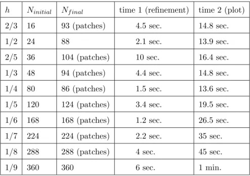
refine-ment step started with 16 points and ended up with 93 points, (b) the level setv0(x, y) = 0 of the last refinement step started with 48 points and ended up with 94 points. In both cases we can see the small patches remaining at the end of the refinement procedure, where the orbital derivative is positive (red areas). . . 35 3.14 The final grid points after the last refinement step started with 24 points
and ended up with 88 points. As we can see, there are no small patches remaining at the end of the refinement procedure. . . 35 3.15 (a) The level setv0(x, y, z) = 0 of the orbital derivative after the last
refine-ment step started with 124 points and ended up with 180 points, (b) and (c) the level set v0(x, y, z) = 0 of the orbital derivative calculated with 728 and 1330 points, where the refinement did not add more points. In all cases we can see some patches remaining at the end (green), wherev0(x, y, z)>0. 39 3.16 The level setv0(x, y, z) = 0 of the orbital derivative calculated with a regular
grid of 2196 points. As we can see there are no patches except for a small neighbourhood, [−0.2,0.2]3, of the equilibrium point (0,0,0). . . 40
4.1 (a) The Delaunay triangulation for X9, where the vertices of the triangles
are our 93 grid points (blue *), (b) the points in P O1 (green *) located in
the areas where the orbital derivative is positive and grouped into 6 clusters based on the triangles they belong to. . . 49 4.2 (a) The clusters centres (black *) calculated using the k-means MATLAB
function, (b) the remaining clusters centres after running the closeness test and removing the 6th centre. . . 50 4.3 The level set v010(x, y) = 0 of the orbital derivative calculated with the new
set of grid pointsX10. As we can see there are still patches remaining where
the orbital derivative is positive. . . 50 4.4 (a) The clusters centres (black *) calculated in the second extension step,
(b) the level set of v110 (x, y) = 0 of the constructed function v11 with the
grid X11 of 102 points. The patches where the orbital derivative is positive
(red areas). . . 51 4.5 (a) The level set v120 (x, y) = 0 of the constructed function v12 with the
final set of grid pointsX12, no areas of positive orbital derivative remaining
except for in a small neighbourhood Enh = [−0.1,0.1]2, of the equilibrium point (0,0), (b) the constructed Lyapunov function v12(x, y) with the first
extension algorithm. . . 52 4.6 (a) The Delaunay triangulation for X1, where the vertices of the triangles
are our 93 grid points (blue *), (b) the points in P O1 (green *) located in
the areas where the orbital derivative is positive and grouped into 8 clusters based on the triangles they belong to. The black (*) represent the centres of the clusters calculated by the k-means function. . . 54 4.7 The level set v20(x, y) = 0 of the orbital derivative calculated with the new
set of grid pointsX2. As we can see there are still patches remaining where
4.8 (a) The Delaunay triangulation for X2, where the vertices of the triangles
are our 93 grid points (blue *), (b) the points in P O2 (green *) located in
the areas where the orbital derivative is positive and grouped into 8 clusters based on the triangles they belong to. The black (*) represent the centres of the clusters calculated by the k-means function. . . 55 4.9 (a) The level sets of the orbital derivative of the constructed function v3
with X3. The (red) patches are the areas where v03(x, y) >0, (b) the level
sets ofv04(x, y) = 0 of the constructed function withX4, with the red patches
where v04(x, y)>0. . . 56 4.10 (a) The Delaunay triangulation forX4, where the vertices of the triangles
are our 93 grid points (blue *), (b) the points in P O3 (green *) located in
the areas where the orbital derivative is positive and grouped into 4 clusters based on the triangles they belong to. The black (*) represent the centres of the clusters calculated by the k-means function. . . 57 4.11 (a) The final set of grid points X5 = 96 points. As we see, there are no
patches where v50(x, y)>0, (b) the Lyapunov functionv5 constructed with
the first modified grid refinement algorithm. . . 57 4.12 (a) The 74 points inP O1(green *) lie in the patches wherev09(x, y)>0, and
the centres to be added to X9 (black *), (b) the level set of v100 (x, y) = 0,
where the red areas are the patches remaining where v010(x, y)>0. . . 60 4.13 (a) The level set of v011(x, y) = 0, the grid points X11 = 100 (blue *) and
the 14 points inP O2 (green *) filling the patches where v11(x, y)>0. We
can see the 2 cluster centres to be added (black *), (b) the level set of v120 (x, y) = 0 with the patches where the orbital derivative is positive. . . . 61 4.14 (a) The level set ofv013(x, y) = 0 and the grid pointsX13= 104 (blue *), as
we can see there are no patches remaining at the end, (b) the constructed Lyapunov function v13(x, y) with the second extension algorithm. . . 62
4.15 (a) The level set of v10(x, y) = 0 of the constructed function v1 after the
last refinement step, started with 48 points and ended up with 60 points, where the (red) patches are the areas wherev10(x, y)>0. (b) The Delaunay triangulation for X1, the points in P O1 (green *) grouped into 8 clusters,
and the centres to be added to X1 (black *). . . 64
4.16 (a) The level set ofv20(x, y) = 0 of the constructed functionv2 with the set
X2 obtained from the first extension step, where the (red) patches are the
areas wherev20(x, y)>0. (b) The level set ofv30(x, y) = 0 of the constructed functionv3 with the set of grid points obtained from the second refinement
step X3. Again, the (red) patches are the areas wherev30(x, y)>0 . . . 65
4.17 (a) The points in P O2 (green *) grouped into 4 clusters, and the cluster
centres (black *), calculated by the subtractive clustering method, (b)the level set of v04(x, y) = 0 of the constructed function v4, where the (red)
patches are the areas where v04(x, y)>0. . . 66 4.18 (a) The level set of v05(x, y) = 0 and the grid points X5 = 96 (blue *), as
we can see there are no patches remaining at the end, (b) the constructed Lyapunov functionv5(x, y) with the second modified grid refinement
algo-rithm. . . 66 4.19 (a) The level set of v30(x, y, z) = 0 (green area), the 13908 points in P O1
where v30(x, y, z) > 0 (red *) and we can see some of the cluster centres as (black *), (b) the level set of v04(x, y, z) = 0 after adding the 36 cluster centres to the grid points, where the green patches are the patches where v40(x, y, z)>0. . . 68 4.20 (a) The 1148 points in P O2 lie inside the patches where v04(x, y, z) > 0
(red *) and cluster centres are shown in (black *), (b) the level set of v50(x, y, z) = 0 after adding the 22 cluster centres to the grid points, where the green patch is the patch where v50(x, y, z)>0. . . 69
4.21 (a) The figure shows where the 952 points inP O3were placed (red *) where
the green area in the middle is the excluded neighbourhoodEnh around the equilibrium (0,0,0), and also shows some of the cluster centres (black *). (b) The level setv70(x, y, z) = 0 of the orbital derivative after the refinement step started with with X6 = 282 and ended up adding 163 points to the
grid, where the small patches (green areas) remaining still have positive orbital derivative. . . 70 4.22 (a) The 40 points inP O4, (red *), lie inside the patches wherev70(x, y, z)>0
and some of the cluster centres are shown as (black *), (b) the level set v80(x, y, z) = 0 of the orbital derivative calculated with X8 = 462 grid
points, as we can see there are no patches remaining at the end. . . 71
5.1 A suitable triangulation inR2 . . . 76
5.2 A square configuration of grid points inR2,h1 is the distance between grid
points in both directions. . . 93 5.3 A body centred square configuration of grid points inR2. . . 94
5.4 (a) The uncovered area (yellow) when choosing L1-norm balls of radius
R1< h1, (b) The square is completely covered withL1-norm balls of radius
R1=h1, centred at the vertices. . . 99
5.5 (a) The uncovered area (yellow) when choosing L1-norm balls of radius
R1 < 12h1, (b) The square is completely covered with L1-norm balls of
radiusR1 = 12h1, centred at the vertices and the centre of the square. . . . 99
5.6 A square [0, h1]2 ⊂ R2 of a square configuration, where (•) are our grid
points, and Ti, i= 1,2 are simplices of the triangulation T. . . 105 5.7 (a) The Delaunay triangulation of the vertices (•) of a squareS= [0, h1]2⊂
R2 of a body centred square configuration, whereh1is the distance between
grid points in both directions, (b) All triangles T1, T2, T3, and T4 satisfy
0 orbital derivative V0(x) =h∇V(x), f(x)i, cf. Definition 1.6.
. temporal derivative ˙x(t) = dtdx(t).
k.k Euclidean vector norm unless otherwise stated.
k.kmax kAkmax= max
1≤i,j≤d|aij|, whereA∈R d×d.
k.k2 kAk2 =Pdi=1Pdj=1(aij)2 12
, whereA∈Rd×d.
A(x0) domain of attraction of x0, cf. Definition 1.5.
δx˜ Dirac’s delta distribution at ˜x∈Rd, i.e., δx˜f(x) =f(˜x).
Bp unit ball of radius 1 under different p-norms.
Enh small neighbourhood around the equilibrium points, which is excluded from the refinement and checking procedures.
f f ∈Cσ(Rd,Rd), right hand side of the ODE ˙x=f(x), cf. (1.1).
hk.kp fill distance under different p-norms.
h1 density ofYod.
K compact set {x∈Rd|V(x)≤R}, where V is a Lyapunov function, cf. Theorem 1.1.
co(K) the convex hull of the set K.
t function with approximates T.
Q Lyapunov function withQ0(x) =−p(x) for x∈A(x0), cf. Theorem 1.3.
q function which approximatesQ.
x+ x+=xforx≥0 and x+= 0 forx <0.
throughout the thesis
First example
The 2-dimensional linear system
˙ x=−x, ˙ y=−y.
which will be visited in Section 2.2 (Example 2.1) and Section 3.2.1 (Example 3.1).
Second example
The 2-dimensional non-linear system ˙ x=−x−2y+x3, ˙ y=−y+12x2y+x3.
which will be visited in the following sections:
Section 3.2.1 (Example 3.2), Section 3.3 (Example 3.5), Section 4.2.2 (Example 4.1), Sec-tion 4.2.4 (Example 4.3), SecSec-tion 5.4 (Example 5.1), SecSec-tion 6.2.1 (Example 6.1), SecSec-tion 6.2.2 (Example 6.3).
Third example
The 2-dimensional non-linear system ˙ x=−x(1−x2−y2)−y, ˙ y =−y(1−x2−y2) +x.
which will be visited in the following sections:
Section 3.2.1 (Example 3.3), Section 3.3 (Example 3.6), Section 4.2.2 (Example 4.2), Sec-tion 4.2.4 (Example 4.4), SecSec-tion 5.4 (Example 5.2), SecSec-tion 6.2.1 (Example 6.2), SecSec-tion 6.2.2 (Example 6.4).
Fourth example
The 3-dimensional non-linear system ˙ x=x(x2+y2−1)−y(z2+ 1), ˙ y=y(x2+y2−1) +x(z2+ 1), ˙ z= 10z(z2−1). which will be visited in the following sections:
Introduction
The determination of the domain of attraction of an equilibrium is an important task in the analysis and derivation of dynamical systems, arising in many practical applications. Since it is difficult to determine the exact domain of attraction analytically, researchers have been seeking numerical algorithms to determine subsets of the domain of attraction. Most of these methods for computing domains of attraction are based on Lyapunov functions, which are functions that decrease along trajectories of the dynamical system. Sublevel sets of Lyapunov functions are positively invariant subsets of the domain of attraction. The construction of such Lyapunov functions, however, is very challenging.
In the last decades, several numerical methods to construct Lyapunov functions have been developed, for a review see [21]. These methods include theSOS (sums of squares) method, which is applicable for polynomial vector fields, introduced in [51] and available as a MATLAB tool box [50]. It constructs a polynomial Lyapunov function bysemidefinite optimization.
The CPA method constructs a CPA (continuous piecewise affine) Lyapunov function using linear optimization [26, 27]. A simplicial complex is fixed and the space of CPA functions which are affine on each simplex is considered. This space can be parameterized by the values on the vertices. The conditions of a Lyapunov function are transformed into a set of finitely many linear inequalities at the vertices, which include error estimates ensuring that the CPA Lyapunov function has negative orbital derivative inside each sim-plex. These linear inequalities are used as constraints of a linear programming problem, which can be solved by standard methods. While in the original method an arbitrarily
small neighborhood of the equilibrium had to be cut out, a revised method can construct a CPA Lyapunov function also near the equilibrium by using a fan-like triangulation near the equilibrium [19].
A different method deals with Zubov’s equation and computes a solution of this partial differential equation (PDE) [9]; the corresponding generalized Zubov equation is a Hamilton-Jacobi-Bellmann equation. This equation has a viscosity solution, a type of weak solution that requires less smoothness than the classical one, which can be approximated using standard techniques after regularisation at the equilibrium, for example one can use piecewise affine approximating functions and adaptive grid techniques [24]. For more details about the theory of viscosity solutions we refer to [5].
The cell mapping approach [30] or set oriented methods [12] divide the phase space into cells and compute the dynamics between these cells; they have also been used to construct Lyapunov functions [25].
The RBF (Radial Basis Function) method, a special case of mesh-free collocation, considers a particular Lyapunov function, satisfying a linear PDE and solves it using
mesh-free collocation [17, 22]. For this method, a set of scattered grid points is used to find an approximation to the solution of the linear PDE. It is computed by solving a linear system of equations.
In this Thesis, we will present our contributions to improve the RBF construction method of Lyapunov functions.
1.1
Outline of the Thesis
The rest of this Chapter gives the necessary background on Dynamical systems, the characterization of a Lyapunov function, and the existence of Lyapunov functions.
InChapter 2, we introduce the construction method of Lyapunov function using radial basis functions. At first, we will explain in detail the radial basis function collocation method for the numerical solutions of PDEs. Then, a description of the construction method for Lyapunov functions, using the RBF collocation method, is provided along with numerical examples.
In Chapter 3, we improve the RBF construction method by combining it with a grid refinement algorithm. This algorithm uses the Voronoi vertices to refine the grid. It shows a great advantage by reducing the required number of grid points as well as the time needed to construct a Lyapunov function, in 2-D and 3-D examples. This part was published in [47].
Chapter 4considers the problem of the early termination of the refinement algorithm without constructing a Lyapunov function. To deal with this issue, we design two modified grid refinement algorithms, which keep refining the grid by using the cluster centres, until a successful construction of a Lyapunov function is achieved.
In Chapter 5, we derive two verification estimates for the negativity of the orbital derivative of the functions constructed with the RBF method. This Chapter is devoted to analyse the effects of different factors on the final formulation of the estimates. The factors considered are: the different norms and the different distributions of grid points, namely the square and the body centred square configurations.
Chapter 6 combines the results of the preceding Chapters in one method calledThe combination method. This method applies the verification estimates to the RBF functions constructed with either a regular grid, the refinement algorithm, or the modified refinement algorithms.
1.2
General Background
1.2.1 Dynamical Systems
Systems motivated by meteorological phenomena, chemical interactions, biological exam-ples and computing systems can be modelled by differential equations. The fact that many differential equations cannot be solved analytically has encouraged many researchers to come up with different numerical methods for solving such equations.
In our study, we will consider the following autonomous system of differential equations, which defines a dynamical system. Let
˙
with f ∈Cσ(Rd,Rd), σ ≥1, d∈ N. The initial value problem ˙x =f(x), x(0) =ξ, has a
unique solutionx(t) which passes through a pointξ ∈Rdat time t= 0. The solutionx(t)
depends continuously on the initial value ξ and is defined for all t∈ I, where 0∈I ⊂R and I is the maximal interval where the solution exists.
The theory of dynamical systems describes how a system changes over time. The following section gives a brief introduction to dynamical systems including some relevant terminolo-gies and definitions.
In [62], a general definition of a dynamical system was given as an evolution rule that defines a trajectory as a function of a single parameter (time) on a set of states (the phase space). Based on this definition we can say that a dynamical system consists of three components :
• Complete metric space (phase space): the set of all states of a given system, X=Rd.
• Time(T): which either be discrete (T=N0) or continuous (T=R+0).
• A function (rule): Stx:X→X, mapping the system’s state at time 0 to time t.
There are two classes of dynamical systems: discrete and continuous. In our study we will only focus on continuous dynamical systems.
Definition 1.1. (Flow Operator for ODE) Define the operator St by Stξ := x(t), where x(t) is the solution of the initial value problem x˙ =f(x), x(0) =ξ ∈Rd for all t∈
R, for which this solution exists.
Assume that the solution exists for all t ≥ 0, then the flow operator St defines a dynamical system.
Definition 1.2. (Continuous dynamical systems) We call (X,R+0, St) a continuous
dy-namical system, if X is a complete metric space and St : X → X is defined for all t ∈ R+0,(t, x) 7→ Stx is a family of continuous mappings with respect to both x and t.
Moreover, we assume that St is a semi-group, i.e.
• S0 =idX.
The simplest solutions of the system (1.1) areequilibriumsolutions, i.e. solutions that do not change in time.
Definition 1.3. (Equilibrium)A pointx0 ∈Rdis an equilibrium point of (1.1), iff(x0) =
0.
If x0 is an equilibrium, then x(t) =x0 is a constant solution for all t≥0.
Stability of an equilibrium point is a very important property in applications. Studying the behaviour of solutions in a neighbourhood of an equilibrium leads us to the fact that not all equilibria are the same. We call an equilibrium stable, if solutions remain near the equilibrium. Moreover, it is called asymptotically stable, if solutions remain near the equilibrium and also they converge to it as time tends to infinity.
Definition 1.4. (Stability of an equilibrium)Let x0 be an equilibrium. x0 is called
1. Stable : if for all >0 there is a δ >0 such that kStx−x0k< for all t ≥0 and
for all x∈Rd such that kx−x
0k< δ .
2. Asymptotically stable : if it is stable and there is a δ0>0such thatkStx−x0k
t→∞
−→ 0
holds for allkx−x0k< δ0.
3. Exponentially asymptotically stable (with exponent−ν <0) : if it is stable and there is a δ0>0 such thatkStx−x0ke+νt t
→∞
−→ 0 holds for all kx−x0k< δ0.
4. Unstable : if it is not stable.
One way of analysing the stability of an equilibrium is by using what is called linear stability analysis, i.e., an analysis based on the sign of the real parts of the eigenvalues of the system matrix. Consider a linear system of differential equations ˙x=Ax, wheref(x) =A and A is an d×d matrix. The equilibrium point of the linear system is asymptotically stable if and only if all real parts of the eigenvaluesλof Aare negative, i.e. Re(λ)<0. If at least one of the eigenvalues has positive real part then the equilibrium is unstable. For non linear systems, the local behaviour near a hyperbolic equilibrium point x0 can
be determined by the behaviour of the linearised system around x0, i.e., ˙x = Ax, where
of the eigenvalues of the matrix Df(x0) have non-zero real parts. Then if all real parts
of the eigenvalues of Df(x0) are negative, the equilibrium is asymptotically stable with
respect to the linearised system and the original non linear system.
Definition 1.5. (Domain of attraction) The domain of attraction of an asymptotically stable equilibrium is the region defined by the set of all solutions which converge tox0, that
is A(x0) := n x∈Rd |S tx t→∞ −→ x0 o (1.2)
One of our main goals is the determination of the domain of attraction of an equilib-rium. We can actually compute a subset of the domain of attraction through sub-level sets of a Lyapunov function.
1.2.2 Lyapunov Functions
The method of Lyapunov functions enables us to determine subsets of the domain of attraction of an asymptotically stable equilibrium through sublevel sets. A function V ∈ C1(Rd,R) is called a Lyapunov function for the equilibriumx0 if it has a local minimum
atx0 and a negative orbital derivative in a neighborhood of x0.
Definition 1.6 (Orbital derivative). The orbital derivative of a function V ∈C1(Rd,R) with respect to (1.1) at a point x∈Rd is defined by
V0(x) =h∇V(x), f(x)i,
where h·,·i denotes the standard scalar product in Rd.
Remark 1.1. The orbital derivative is the derivative along solutions: with the chain rule we have d dtV(Stx) t=0=h∇V(Stx), d dtStxi t=0=h∇V(x), f(x)i=V 0 (x). (1.3)
The following theorem shows how Lyapunov functions are used to find subsets of the domain of attraction; note that the requirement of the local minimum at x0 is a
consequence of the assumptions. The theorem states that sublevel sets of a Lyapunov function are positively invariant subsets of the domain of attraction, see e.g. [17, Theorem 2.24].
Theorem 1.1. Let x0 ∈ Rd be an equilibrium of x˙ = f(x) with f ∈ C1(Rd,Rd). Let
V ∈C1(Rd,R) be a Lyapunov function and letK⊂Rd be a compact neighbourhood ofx0.
Furthermore, let
1. K =x∈Rd|V(x)≤R for anR∈R, i.e., K is a sublevel set of V.
2. V0(x)<0 for all x∈K\ {x0}, i.e., V is decreasing along solutions in K\ {x0}.
Thenx0 is asymptotically stable,K is positively invariant andK ⊂A(x0)holds. Moreover,
V(z)> V(x0) holds for all z∈K\{x0}.
Existence of Lyapunov functions
Over the last century, the Lyapunov theory of dynamical systems has been the most pow-erful contribution used for analysing the stability of different types of dynamical systems, which are mathematically modelled by ordinary differential equations. In 1892, Alexander Lyapunov introduced two methods: Lyapunov’s indirect method and Lyapunov’s direct method.
The direct method of Lyapunov (also called Lyapunov’s second method), is a technique that allows us to investigate the stability properties of a given system without solving it explicitly. The idea of this method is to find a functionV, that is strictly decreasing along a system’s trajectories and these trajectories must eventually converge to the equilibrium point of the system. If such functionV exists, then it is called a Lyapunov function and the equilibrium point is asymptotically stable.
However, the difficulty of Lyapunov’s direct method lies in finding a suitable functionV. This problem gives rise to the converse concept of Lyapunov’s direct method; i.e., given that an equilibrium is stable or asymptotically stable, does a suitable Lyapunov function V exist? And if it does exist, how it can be constructed ?
Simply, the converse Lyapunov theorems are results that guarantee the existence of a Lya-punov function under some stability conditions.
In the case of linear systems, Lyapunov answered the converse question via his indirect methods, which says very briefly: if a linear system (I) ˙x=Ax, x∈Rd has an asymptot-ically stable origin, then by [44] there exists a unique positive definite solutionP ∈Rd×d,
Lyapunov’s indirect method, the quadratic functionV(x) =x|P xis a Lyapunov function for (I).
Consequently, a local Lyapunov function can be constructed for non-linear systems by considering the linearisation around the equilibrium point. However, Lyapunov’s original work did not guarantee the existence of Lyapunov functions for non-linear systems. The first converse theorem in the general case was due to Persidskii [52]. Then, in 1949 Massera provided the first converse theorem for asymptotic stability [45]. Many authors have developed Massera’s result in several directions to answer the converse questions re-lated to different cases, for an overview see [36] and [19].
Although these converse theorems guarantee the existence of Lyapunov functions, its main drawback is that they do not provide a method to construct Lyapunov functions for non-linear systems explicitly.
In our study, we will assume thatx0is an exponentially stable equilibrium and we will
con-sider two classes of Lyapunov functions, such thatV0(x)<0 holds for allx∈A(x0)\{x0}.
We will characterize them by equations for their orbital derivativesV0(x); these are linear first order partial differential equation (PDE) forV. Both functions have the same degree of smoothness as f, i.e. they areCσ functions.
• The first class are Lyapunov functionsT, which satisfy the equation
T0(x) =−¯c,
where ¯c >0 is a given constant. Note, however, that the function T is not defined atx0 and fulfills limx→x0T(x) =−∞.
To prove the existence ofT, we need first to define a non-characteristic hypersurface.
Definition 1.7. (non-characteristic hypersurface [17, Definition 2.36]). Consider
˙
x = f(x), where f ∈ Cσ(Rd,Rd), σ ≥ 1. Let h ∈ Cσ(Rd,R). The set Ω ⊂ Rd is called a non-characteristic hypersurface if
1. Ω is compact,
2. h(x) = 0 if and only if x∈Ω, 3. h0(x)<0 holds for allx∈Ω, and
Theorem 1.2. (Existence of T [17, Theorem 2.38]). Letx˙ =f(x), f ∈Cσ(Rd,Rd),
σ ≥ 1. Let x0 be an equilibrium such that −ν < 0 is the maximal real part of all
eigenvalues of Df(x0).
LetΩbe a non-characteristic hypersurface. Then there is a functionθ∈Cσ(A(x0)\{x0},R) satisfying
Stx∈Ω⇔t=θ(x).
Furthermore, θ0(x) =−1 andlimx→x0θ(x) =−∞.
For all¯c∈R+and all functionsH∈Cσ(Ω,R)there is a functionT ∈Cσ(A(x0)\{x0},R) satisfying
T0(x) =−¯c for all x∈A(x0)\{x0} and
T(x) =H(x) for all x∈Ω.
Moreover, limx→x0T(x) =−∞.
• The second class are Lyapunov functions which satisfy
Q0(x) =−kx−x0k2
or a similar right-hand side.
Before stating the existence theorem for this class of Lyapunov functions, we first define positive definite functions through class K functions.
Definition 1.8. [20, Definition 2.7].
1. A continuous function α: [0,+∞[→[0,+∞[is said to be of classK ifα(0) = 0
and α is strictly monotonically increasing.
2. Let U be a neighborhood of the origin, and let p:U →R be a locally Lipschitz continuous function. We say that p is a positive definite function if p(0) = 0
and there exists a class K function α such that p(x)≥α(kxk2) for all x∈ U.
Theorem 1.3. (Existence of Q). Let x0 be an equilibrium of x˙ = f(x) with f ∈
Cσ(Rd,Rd), σ ≥ 1, such that the maximal real part of all eigenvalues of Df(x0)
is −ν < 0. Let p ∈ Cσ(Rd,R) be a positive definite function. Then there exists a Lyapunov function Q∈Cσ(A(x0),R) with Q(x0) = 0 such that
holds for allx∈A(x0). If sup
x∈A(x0)
kf(x)k<∞, then
KR:={x∈A(x0)|Q(x)≤R}
is a compact set inRd for all R≥0.
Theorem 1.3 follows from [20, Theorem 2.8]. For more details and background of Theorems 1.2 and 1.3, see [17, Section 2.3].
Construction of Lyapunov
Functions using RBF
2.1
Numerical solutions for PDEs using the Radial Basis
Functions collocation method
Meshless collocation based on Radial Basis Function is an effective tool to solve linear PDE’s. It has outstanding properties, such as approximating arbitrarily scattered data in multidimensional space as well as providing high order of accuracy which have made it a preferable method for the numerical solutions of PDEs. For a general introduction to Meshless collocation, in particular Radial Basis Functions, see [8, 61]. For the application of RBF to the construction of Lyapunov functions, see [17], where details for the following overview of the method can be found, as well as [22].
A Radial Basis Function is a real-valued function whose value depends only on the distance from the origin i.e., Ψ(x) =ψ(kxk), wherek · kdenotes the Euclidean norm inRd.
There is a one-to-one correspondence between a Radial Basis Function, or more generally kernel, and its Reproducing Kernel Hilbert Space (RKHS), see [61]. The approximate solution of the PDE will be a norm-minimal interpolant in the RKHS; in our brief overview, however, we do not discuss this relation further, the interested reader is referred to [22].
In the following section we will introduce a family of compactly supported Radial Basis Functions that enables us to approximate functions with certain smoothness, i.e. not
necessarily C∞. Note that the corresponding RKHS is a Sobolev space with equivalent norm.
The Wendland functions, introduced by Wendland [60], are compactly supported Ra-dial Basis Functions, which are polynomials on their support.
Definition 2.1 (Wendland Functions). Let l∈N, k∈N0. We define by recursion
ψl,0(r) = (1−r)l+ (2.1) and ψl,k+1(r) = 1 Z r tψl,k(t)dt (2.2)
for r ∈R+0. Here we set x+=x for x≥0 and x+ = 0 for x <0.
If we fix the parameter l := bd2c+k+ 1 depending on the space dimension d and the parameter k, then the function Ψ(x) =ψl,k(ckxk) with c > 0 is a C2k function with compact support. For dimensions d = 2 or d = 3, we give some Wendland functions in the following table.
k ψl,k
1 ψ3,1(cr) = (1−cr)4+(4cr+ 1)
2 ψ4,2(cr) = (1−cr)6+(35c2r2+ 18cr+ 3)
3 ψ5,3(cr) = (1−cr)8+(32c3r3+ 25c2r2+ 8cr+ 1)
4 ψ6,4(cr) = (1−cr)10+(429c4r4+ 450c3r3+ 210c2r2+ 50cr+ 5)
Table 2.1: The Wendland functionsψ3,1(cr),ψ4,2(cr),ψ5,3(cr) andψ6,4(cr) with l=k+ 2
and a scaling parameter c >0. Note that these functions are the Wendland functions of Definition 2.1 up to a constant.
Now let us consider a general linear partial differential equation of the form
Lu=g on Ω⊂Rd, (2.3)
whereL is a linear differential operator of the form
Lu(x) = X
|α|≤m
In our case, the differential operatorLwill be given by the orbital derivative of a function V with respect to system (1.1), namely
LV(x) :=h∇V(x), f(x)i= d X
j=1
fj(x)∂jV(x) =V0(x) (2.5)
The operatorLin (2.5) is a first order differential operator of the form (2.4) withcej(x) =
fj(x).
Let XN ={x1, x2, . . . , xN} ⊂ Ω be a set of N pairwise distinct points which are no equilibria. DefineDirac’s delta-operator δ by δy0g(x) =g(y0). Then we have
(δxk◦L)
xV(x) =LV(x
k) =V0(xk),
where the superscriptxdenotes the application of the operator with respect to the variable x. The approximant v:Rd→RofV will be given by
v(x) = N X k=1 βk(δxk◦L) yΨ(x−y) (2.6)
where Ψ(x) is the Radial Basis Function. The coefficientsβk are determined by claiming that the interpolation condition
(δxj◦L)
xV(x) = (δ xj◦L)
xv(x)
is satisfied for all grid points xj ∈XN, or in other words that the PDE is satisfied at all pointsxj ∈XN. This will lead to a linear system forβ
Aβ =α (2.7)
If the points xj are pairwise distinct and no equilibria, then the symmetric matrix A is positive definite, so in particular non-singular. Hence, the system has a unique solution β. The interpolation matrix entries ofA= (ajk)j,k=1,...,N are given by
ajk = (δxj◦L)
x(δ xk◦L)
yΨ(x−y)
and the right-hand sideα= (αj)j=1,...,N is given by
αj = (δxj◦L)
xV(x) =LV(x
j) =V0(xj)
Finally, we calculate the approximant v(x) and its orbital derivative v0(x), using the following formulas, by evaluating and taking the orbital derivative of (2.6).
v(x) = N X k=1 βkhxk−x, f(xk)iψ1(kx−xkk), (2.8) v0(x) = N X k=1 βk ψ2(kx−xkk)hx−xk, f(x)ihxk−x, f(xk)i −ψ1(kx−xkk)hf(x), f(xk)i , (2.9)
whereψ1 andψ2 are defined as:
ψ1(r) = d drψ(r) r , forr >0 (2.10) ψ2(r) = d drψ1(r) r forr >0 0 forr= 0 (2.11)
Note thatψ1 can be continuously extended to 0.
Remark 2.1 (The value of ¯c). Changing the value of ¯c >0 has the effect of multiplying the solution β of the linear system Aβ=α by a positive constant. As a consequence also the value of the approximant v and its orbital derivative v0 will be multiplied by the same positive constant. This means that the areas of the phase space, where v0 is positive, are independent of the value of ¯c.
Indeed, this follows from Aβ=α=−(1,1, . . . ,1)T ¯c, since the interpolation matrix A
is independent of the value of c¯and from formulas (2.8) and (2.9).
The following error estimate was given in [22, Corollay 4.11]. Note, thatW2τ(Ω) denotes the usual Sobolev space on Ω⊂Rd.
Theorem 2.1. Denote by k the smoothness index of the compactly supported Wendland function and fix l := bd2c+k+ 1. Let k > 12 if d is odd or k > 1 if d is even. Set
τ = k+ (d+ 1)/2 and σ = dτe. Consider the dynamical system defined by (1.1), where
f ∈ Cσ(Rd,Rd). Let x0 be an exponentially stable equilibrium point of (1.1). Let f be
bounded in A(x0) and denote by V ∈ W2τ(A(x0),R) the Lyapunov function satisfying
V0(x) =−kx−x0k2.
The reconstructionv of the Lyapunov functionV with respect to the operator (2.5) and a compact set K ⊂Ω :={x∈A(x0)|V(x)≤r}, r >0, satisfies
kv0−V0kL∞(Ω) ≤Chk−12kVk
where h:= supx∈Ωminxj∈XNkx−xjkdenotes the fill distance, i.e. the maximum distance
which a point in Ωcan have from the nearest point in XN.
Remark 2.2. The set K in the theorem above can be any compact subset of A(x0) as r
can be chosen so large that the sublevel setΩofV satisfiesΩ⊃K. A similar statement for the function satisfying V0(x) =−¯c follows also from [22, Corollay 4.11], but with no data sites on the boundary. Note, however, that in this case the function satisfying V0(x) =−¯c
is only unique up to a constant, the error estimates on the orbital derivative, however, still hold.
The error estimate (2.12) implies that the approximant v of the Lyapunov func-tion V is actually a Lyapunov function, i.e. satisfies v0(x) < 0, if the grid is dense enough. Let us make this more precise: by choosing the fill distance h so small that Chk−12kVk
W2k+(d+1)/2(Ω)≤for a given >0,
1. forV0(x) =−kx−x0k2 we have with|V0(x)−v0(x)| ≤, hence
v0(x)≤V0(x) +=−kx−x0k2+ <0 if kx−x0k2 > . (2.13)
2. forV0(x) =−¯c we have with|V0(x)−v0(x)| ≤, hence
v0(x)≤V0(x) +=−¯c+ <0, if <¯c. (2.14)
Remark 2.3. In both cases, the approximation may fail to have negative orbital derivative near the equilibrium x0; in the first case the error estimate requires kx−x0k2 > , and
in the second case the function V is not defined in x0. If the equilibrium is exponentially
stable, one can use the Lyapunov function of the linearised system, the so-called local Lyapunov function, to deal with this small neighborhood of x0, for details see [17], or a
modified method, see [18]. In this thesis, we will not deal with this local problem in more detail.
The error estimate uses the fill distance as a measure; hence, we are led to choose a uniformly fine grid. In examples, however, it turns out that an approximation with negative orbital derivative can be achieved with fewer points using a non-uniform grid. Moreover, the goal is not necessarily to have a good approximation ofV, but to construct a function with negative orbital derivative. For example, when approximating the solution of V0(x) =−kx−x0k2, a larger error is permissible for points far away from the equilibrium.
2.2
Steps of the Construction Method
The construction method is based on considering the Lyapunov functions satisfying the PDEs stated in Section 1.2.2. We will explain this construction method in an example.
Example 2.1. Consider the simple linear system
˙ x=−x, ˙ y=−y.
The system has one asymptotically stable equilibrium x0 = (0,0). Now we will go
through the steps of the method.
• Choose a Radial Basis Function Ψ(x) = ψl,k(ckxk), here we choose the Wendland
functionψ6,4 withc= 1.
• Choose a grid XN ={x1, x2, . . . , xN} ⊂R2, containing no equilibrium point. Here, we fix a regular grid XN = {(x, y) ∈ R2 | x, y ∈ {0,±h,±2h, . . . ,±1}} \ {(0,0)}, where h >0 is the distance between points inx- and y-direction and will be specified below.
• Use the RBF method to approximate the Lyapunov function V =T which satisfies
T0(x) =−1 by the approximant v and then calculate its orbital derivatives v0 using (2.8) and (2.9).
• From the ansatz of the Lyapunov function V, we know that the orbital derivative is negative at every point in our grid, i.e., v0(xi)<0 for all xi ∈XN ⊂R2, but there may be points in[−1,1]2, where the orbital derivative is positive. The error estimate tells us that if h is small enough, the orbital derivative will be negative except for a small neighborhood of the equilibrium. Hence, we start with a certain h, and check the sign of the orbital derivative at the points between the grid points. If we have points where v0(x) > 0, we need a finer grid. Therefore, we choose h smaller and smaller until we have v0(x) <0 for all points in the desired area. In this example, we used h= 1/6, resulting in N = 168 points.
• Find a sublevel set K of the Lyapunov function (the approximant) v of level R∈R
of attraction A(x0). Figures 2.1 and 2.2 show the functionsv and v0 as well as level
sets ofv.
(a) The constructed Lyapunov function v(x, y).
(b) Level sets ofv(x, y).
Figure 2.1: (a) shows the constructed Lyapunov function vand (b) different sublevel sets of v for different values ofR, which are subsets of the domain of attraction.
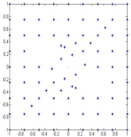
Figure 2.2: The orbital derivative v0(x, y) of the constructed Lyapunov function v; note that v0(x)≈ −1, except for a small neighborhood of the origin.
During the calculations of the Lyapunov function v we may find some points with positive orbital derivatives. This occurs because either the grid we have chosen is not fine enough, or the grid points do not all lie in the domain of attraction. We cannot exclude
the second case, so we use a finer grid to calculate the Lyapunov function v and see if the problem will be solved. However, instead of using a regular, finer grid, the question is whether the refinement can be done more efficiently by using an irregular grid with fewer points. Our goal is to have a fine grid but to avoid expensive computations which are caused by refining the whole area rather than only the parts where we need to add more points. Therefore, we combine this construction method with a refinement algorithm.
Grid Refinement Algorithm
For the numerical solution of partial differential equations (PDE) using mesh-free methods, adaptive refinement techniques play an important role in achieving better accuracy with the minimum number of points. This will be done by only refining (adding more points to) the areas where the solution of the PDE has rapid variations [33, 54, 7, 2]. Since the mesh-free methods, including the RBF approximation method, do not require special connectivity between points, the procedure of adding (or removing) points becomes easy and convenient.
During the last two decades, scientists in the field of scientific computation and engi-neering have paid a considerable attention to the development of adaptive algorithms for mesh-free methods [13, 39, 56, 43, 15, 3, 42, 49]. Some of the node refinement strategies in the literature include: applying the adaptive mesh refinement (AMR) algorithm to place overlapping refined grids recursively over the regions specified by an error estimator. the refinement procedure stops after the spatial discretization error of the radiative transport equation (RTE) has reached a sufficient level [34]. On the other hand, [38] used a phase indicator to refine nodes in the liquid phase, (by adding four symmetric nodes around the refined node), which needs higher node distribution density comparing to the solid one in solving thermo fluid problems with phase change [38]. Moreover, a local refinement using a local Delaunay triangulation algorithm and other adaptive techniques were presented in [41].
For the RBF construction method, introduced in the previous Chapter, we will combine it with a grid refinement algorithm, aiming for a successful construction of Lyapunov
functions with fewer collocation points and less computation time than the original method
3.1
The Refinement Algorithm
Our proposed algorithm is recursive and usesVoronoi diagrams. In each step, given a grid, we generate a Voronoi diagram for our grid points, then we consider the Voronoi vertices of each cell of this diagram as possible points to be added to the grid. Finally, we run a test on each Voronoi vertex and decide whether we add the point to the grid or not.
We have used Voronoi vertices as new possible points for our grid since they are equidistant to three or more previous grid points, and thus lie “in between” the previous grid points. Consequently, we guarantee not to add points that are too close to each other, which would lead to a singular interpolation matrixA of the linear system (2.7).
We start the first section of this Chapter by a brief introduction to the Voronoi dia-grams and its dual structure, the Delaunay triangulation, then describe the strategy of the refinement algorithm. In the second section, we discuss the issue of the unsuccessful termination of the refinement algorithm. The contents of this Chapter were published in [47].
3.1.1 Voronoi Diagram and Delaunay Triangulation
Voronoi diagrams and Delaunay triangulations have enormous applications in different scientific fields, especially in mesh generation and nodes insertion procedures. Sibson [58] developed an interpolation method based on Voronoi diagrams, the method is known as natural neighbour interpolation method. Moreover, there is a refinement algorithm called Ruppert’s Delaunay refinement algorithm [57]. Some recent works include [35], presenting a refinement procedure to develop the gradient smoothing method using Delaunay trian-gulation for the adaptive analysis in solid mechanics, and [64], where a Voronoi neighbour criterion is used to construct the adaptive radial point interpolation method. Voronoi di-agrams have also been used in kernel-based adaptive particle methods for numerical flow simulation [31], and for a thinning algorithm in multistep interpolation with Radial Basis Functions [14].
A Voronoi diagram is a geometric structure that divides a d-dimensional space into cells based on the distance between sets of points in the space [55]. Many algorithms have been proposed for computing Voronoi diagrams. The fundamental and most popular ones include: The Divide and Conquer algorithm and Fortunes’s Sweep Line algorithm [6]. For the purpose of explaining the structure of Voronoi diagrams, we will explain a very simple but less efficient algorithm using perpendicular hyperplanes.
Figure 3.1: The Voronoi diagram for a set of sites (green o) with a Voronoi region, Voronoi edge and Voronoi vertex (red *).
Let S = {s1, s2, . . . , sn} ⊂ Rd be a set of n arbitrarily distributed and distinct sites
(points) in Rd. The perpendicular bisector algorithm works as follows: for each pair of
sites inS we construct a perpendicular hyperplane to the line segment joining these sites. At the end of this process, we will have intersections of finitely many hyperplanes which build up cells, with a convex polygon structure, known asVoronoi regions. The boundaries of each region are called Voronoi edges and the intersections of Voronoi edges are called
Voronoi vertices. For more details see [6, 37, 32].
Mathematically, the Voronoi region of a point si inS is defined by
Vi= n \ j=1,j6=i n x∈Rd|kx−sik<kx−sjk o ,
a Voronoi region Vi the Euclidean distance of x to the site si, which is also inside the region, is smaller than the Euclidean distance ofx to any other site sj.
Remark 3.1. As the Voronoi region is the intersection of finitely many hyperplanes, each Voronoi region is a convex polygon.
Delaunay Triangulation:
Delaunay triangulation is the dual structure of a Voronoi diagram. The relation be-tween them is simply that the sites of the Voronoi diagram are the vertices of the Delaunay triangulation and vice versa. See figure 3.2.
It is defined as a partition of the convex hull of S intoO(ndd2e) d-simplices in which the
circumsphere, the sphere passing through the vertices of a simplex, of each d-simplex is empty, i.e., there are no sites ofS in its interior. The Delaunay triangulation is uniquely defined, if all vertices are in a so called general position, i.e., no more than d+ 1 vertices lie on a common sphere [10, Theorem 2.11].
Figure 3.2: The Delaunay triangulation of the Voronoi diagram in figure (3.1). The sites of the Voronoi diagram (green o) are the vertices of the Delaunay triangulation.
3.1.2 The Algorithm Strategy
The first step of the refinement process starts by constructing an RBF approximantv1with
a coarse grid of collocation pointsX1. The Voronoi diagram forX1 will place the Voronoi
vertices in between the grid points in X1, making them potential points to be added to
the grid. Therefore, we check the sign of the orbital derivativev10 at each Voronoi vertex. Then, we add all the vertices with positive orbital derivative to X1 and ignore the ones
with negative orbital derivative. By the end of this step, we are obtaining a new set of grid pointsX2 =X1∪ {Voronoi vertices with positive orbital derivative}, as well as a new
approximant v2 forX2.
The algorithm will be repeating this step until it terminates as no new points are added. The implementation of the refinement algorithm follows the following steps.
1. Fix a compact neighbourhoodK⊂Rdof the equilibriumx
0and a Radial Basis
Func-tion. Letn= 1 and start with an initial set of grid pointsX1 ={x(1)1 , x (1) 2 , . . . , x
(1)
N1} ⊂
K, not containing any equilibrium.
2. Calculate a Lyapunov function vn using the RBF method with the grid Xn = {x(1n), x2(n), . . . , x(Nnn)}. In the following steps, we drop the superindex (n) if it is clear in which step we are.
3. Generate Voronoi vertices, Yn = {y1, y2, . . . , yMn} ⊂ R
d, for the grid points X n. Exclude points inYnwhich are equilibria, or which lie in a small neighbourhoodEnh of an equilibrium or which lie outsideK.
4. Run a test on each vertex in the set Yn and check whethervn0(yj)<0 (yj ∈Yn−) or vn0(yj)≥0 (yj ∈Yn+), wherej= 1, . . . , Mn and Yn=Yn−∪Yn+.
5. Define new grid Xn+1 =Xn∪Yn+.
6. n→n+ 1, repeat the steps 2. to 5. untilY+
n =∅.
3.2
Numerical Examples
The application of the refinement algorithm on numerical examples has a general structure as follows: the starting grid of the refinement process is a coarse and equidistant grid of
collocation points with fill distance h. Then, we run the refinement algorithm until we successfully construct a Lyapunov functionv. After that, we fix a checking grid Xcheck of sizehcheck, which is smaller thanh, to check the negativity of the orbital derivative of v. However, we will provide a rigorous estimate for checking the sign ofv0 in Chapter 5. It is important to mention that usually there will be a small neighbourhood Enh around the equilibrium point, which is excluded from the refinement and the checking procedures as we cannot expect v0 to be negative here, see Remark 2.3.
3.2.1 Two-dimensional Examples
Example 3.1. Consider the system from Example 2.1. We will explain the refinement al-gorithm starting with a coarse equidistant gridX1={(x, y)∈R2 |x, y∈ {0,±h, . . . ,±1}}\
Enh, where Enh={(0,0)} and h= 1, i.e. N1= 8 points.
• The first step of the algorithm n = 1: We start with an initial grid X1 = {xi}8i=1
and calculate the Lyapunov function v1 on the grid X1. Figure 3.3 (a) shows the
level setv10(x, y) = 0 with the area wherev10(x, y)>0 in green. We can also see the Voronoi diagram for our grid points and the circled Voronoi vertices which will all be added to the set X1, since they are all located in the green area. In this case, we
have Y1+ = Y1 and Y1− =∅, i.e. all four new points (the equilibrium is not part of
Y1) have positive orbital derivative and will be added to the grid.
• The second step of the algorithm n = 2: Our new set of grid points is now X2 =
X1∪ {yj}4j=1. Figure 3.3 (b) shows the level setv20(x, y) = 0. Again, we generate a
Voronoi diagram for the set X2 and determine the Voronoi vertices to be added to
the existing grid points, see Figure 3.3 (b).
• The third step of the algorithm n = 3: The new set of grid points is X3 = X2 ∪
{yj}12j=1. After going through the same steps again we show in Figure 3.4 (a) the
grid and level set v03(x, y) = 0.
• After the fourth step, the set Y4+ =∅ and the algorithm terminates as all Voronoi vertices have negative orbital derivative. Figure 3.4 (b) shows the final set of grid points X4 =X3∪ {yj}12j=1 and no more areas with positive orbital derivative (green
(a) The first stepn= 1 with 8 grid points. (b) The second step n = 2 with 12 grid points.
Figure 3.3: The first two steps, n= 1,2, of the refinement algorithm. Both figures show the level setv0(x, y) = 0, which divides the region into areas withv0(x, y)>0 (green), and areas withv0(x, y)<0 (white). The grid points are blue * and the Voronoi diagrams with Voronoi vertices (red o) are shown.
areas). Thus, we have found a Lyapunov function and will now be able to determine sublevel sets, which are subsets of the domain of attraction. We plot the graph of the Lyapunov function in Figure 3.5 (a) and its sublevel sets in Figure 3.5 (b).
To show that v0 is negative, we have checked that the sign ofv0(x, y) is negative on the gridXcheck={(x, y)|x, y∈ {0,±hcheck,±2hcheck, . . . ,±1}} \ {(0,0)}withhcheck= 10−3.
Note that, in Chapter 5, we will provide a more reliable method to check the negativity of the orbital derivative over a compact set K.
When solving the same example with a regular grid in Example 2.1, we neededN = 168 points, whereas with the refinement algorithm we have constructed a Lyapunov function with a grid of only N4 = 40 points, hence we have reached our goal of having a dense
enough grid with fewer points. The sublevel sets of the Lyapunov function with the refinement algorithm are similar to those that we obtained with the regular gridN = 168, see Figures 2.1 (b) and Figure 3.5 (b).
After successfully testing the refinement algorithm on a linear system, we will now examine it on a nonlinear one.
(a) The third step of the refinement algo-rithm showing the level setv03(x, y) = 0,
in green the areas wherev03(x, y)>0. The
24 grid points ofX3(blue *) and Voronoi
vertices (red o) to be added to setX3.
(b) The final setX4 of 40 grid points (red
*) after the refinement algorithm has ter-minated – no areas wherev04(x, y)>0 are
left.
Figure 3.4: (a) shows the third step of the refinement algorithm, and (b) shows the final set of grid points with no areas of positive orbital derivative.
(a) The constructed Lyapunov function v4(x, y).
(b) Different sublevel sets ofv4(x, y).
Figure 3.5: (a) The constructed Lyapunov functionv4(x, y) with the refinement algorithm
Example 3.2. Consider the non-linear system [22, Example 4.3] ˙ x=−x−2y+x3, ˙ y=−y+12x2y+x3.
The system has an asymptotically stable equilibrium at (0,0).
For this example, we approximate the Lyapunov function satisfying V0(x) =−kxk2. We
have used the Wendland function ψ6,4 with c=1 and started with the grid X1 ={(x, y)∈
R2 | x, y ∈ {0,±h, . . . ,±1}} \Enh, where Enh = [−0.1,0.1]2 and h = 0.2, i.e. N1 = 24
points. Figure 3.6 (a) shows the region where v01(x, y) > 0 (green) and Figure 3.6 (b) shows the Voronoi diagram and vertices Y1. The points marked with red o (14 points)
have positive orbital derivative and form the setY1+, these are the points that will be added to the previous grid. On the other hand, the two blue points (blue *) have negative orbital derivative and form the set Y1−, thus will not be added to our grid points.
(a) The starting grid withN1= 24 points. (b) The Voronoi verticesY1 =Y1+∪Y − 1 .
The points in the green area (red o) form the setY1+ and will be added to our
exist-ing set X1 of grid points; there are two
Voronoi vertices lying in the white set (blue *), they form the set Y1− and will not be added to the grid.
Figure 3.6: Both figures show the level setv10(x, y) = 0, which divides the region into areas with v01(x, y)> 0 (green), and areas withv10(x, y) <0 (white). The grid points N1 = 24
Figure 3.7 (a) shows the level sets of the approximation v2, using the refined grid
X2=X1∪Y1+; the orbital derivative ofv2 for all points of X2 is negative by construction.
After four refinement steps, the algorithm terminates with 88 grid points and the final function satisfies v40(x, y) < 0 everywhere; no green areas (where v40(x, y) > 0) occur in Figure 3.7 (b). To show that v40 is negative, we have checked that the sign of v40(x, y) is negative on the grid Xcheck = {(x, y) | x, y ∈ {0,±hcheck,±2hcheck, . . . ,±1}} \Enh with hcheck= 10−3.
(a) The level setv20(x, y) = 0 after the first
refinement procedure, recalculated on the new setX2 ofN2= 38 grid points. Areas
wherev20(x, y)>0 are shown in green.
(b) The grid pointsN4= 88 after the
ter-mination of the refinement algorithm.
Figure 3.7: (a) The second step of the refinement algorithm and (b) the final step of the refinement algorithm: no areas with positive orbital derivative are left.
Figure 3.8 (a) shows the graph of the constructed Lyapunov function v4(x, y), and
Figure 3.8 (b) shows some of its sublevel sets. To construct a Lyapunov function with a regular grid which has negative orbital derivative on Xcheck, we need a grid of N = 360
points.
Example 3.3. Consider the system [17, Example 2.10]
˙ x=−x(1−x2−y2)−y, ˙ y=−y(1−x2−y2) +x.
(a) The constructed Lyapunov function v4(x, y) with the refinement algorithm.
(b) Different sublevel sets ofv4.
Figure 3.8: (a) The constructed Lyapunov functionv4(x, y) with the refinement algorithm
and (b) different sublevel sets ofv4.
In this example, we have used the Wendland function ψ6,4 with c = 1 and approximated
the Lyapunov function satisfying T0 = −1. We start our refinement algorithm with an initial set of regular grid points X1 = {(x, y) ∈ R2 | x, y ∈ {0,±h, . . . ,±0.9}} \Enh,
where Enh = [−0.1,0.1]2 and h = 0.36, i.e. N1 = 36 points distributed on a compact set
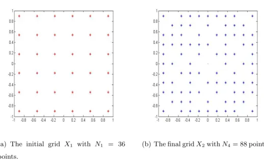
K = [−0.9,0.9]2, see figure 3.9 (a). After performing four refinement steps, the algorithm successfully constructs a Lyapunov function v4 with N4 = 88 points, see figure 3.9 (b).
The constructed function v4 satisfies v40(x, y) < 0 on a checking grid Xcheck = {(x, y) | x, y∈ {0,±hcheck,±2hcheck, . . . ,±0.9}} \Enh with hcheck = 10−3. Figure 3.10 (a), shows
the Lyapunov function v4 constructed with the final set of grid points obtained with the
refinement algorithmN4 = 88points. Moreover, figure 3.10 (b), displays different sublevel
sets of v4.
Note that, the domain of attraction of this system is given by A(0,0) ={(x, y) ∈R2 |
x2 +y2 < 1}, so K actually is not a subset of the domain of attraction. As usually the domain of attraction is not known in advance, this is a realistic situation, and even in this situation, the refinement algorithm has worked well.
(a) The initial grid X1 with N1 = 36
points.
(b) The final gridX2withN4= 88 points.
Figure 3.9: (a) shows the distribution the initial grid points, (b) the distribution of final grid points after the last refinement step.
(a) The constructed Lyapunov function v4(x, y) with the refinement algorithm.
(b) Different sublevel sets ofv4.
Figure 3.10: (a) The constructed Lyapunov functionv4(x, y) with the refinement algorithm
and (b) different sublevel sets ofv4.
3.2.2 Three-dimensional Example
Example 3.4 (Three-dimensional system). Consider the 3-dimensional system given in [17, Example 6.4]
˙ x=x(x2+y2−1)−y(z2+ 1), ˙ y =y(x2+y2−1) +x(z2+ 1), ˙ z= 10z(z2−1).
The system has an exponentially stable equilibrium at(0,0,0)and its domain of attraction is given by
A(0,0,0) ={(x, y, z)∈R3|x2+y2<1,|z|<1}.
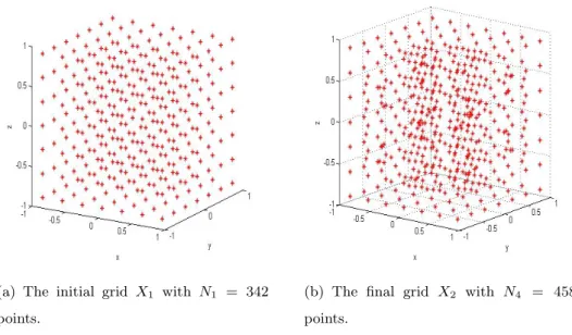
In [17, Example 6.4], an RBF approximation with 137points resulted in a large area near the equilibrium with positive orbital derivative; larger than the set [−0.2,0.2]3, which is later excluded in our example. With a modified algorithm, using the Taylor polynomial at the equilibrium, this was overcome in [17, Example 6.4].
As generally the domain of attraction is not known, we have chosen to use a grid in the set K = [−0.9,0.9]3, which is not a subset of the domain of attraction, but also does not include other invariant sets. This is a more realistic, but also more challenging test case for the method.
(a) The initial grid X1 with N1 = 342
points.
(b) The final grid X2 with N4 = 458
points.
Figure 3.11: (a) shows the distribution the initial grid points, (b) the distribution of final grid points after the last refinement step.
We choose the Wendland function ψ6,4 with c= 0.6. We have started with a regular


![Table 3.2: The number of grid points and the values of h we have used to construct Lyapunov functions for Example 2.10 of [17]](https://thumb-us.123doks.com/thumbv2/123dok_us/1455388.2694737/55.892.170.680.489.739/table-number-points-values-construct-lyapunov-functions-example.webp)
