Boston University
OpenBU http://open.bu.edu
BU Open Access Articles BU Open Access Articles
2017
Multiple measures of historical
intergenerational mobility: Iowa
1915 to 1940
This work was made openly accessible by BU Faculty. Please share how this access benefits you.
Your story matters.
Version
Citation (published version): JJ Feigenbaum. 2017. "Multiple Measures of Historical
Intergenerational Mobility: Iowa 1915 to 1940." Economic Journal, https://hdl.handle.net/2144/27523
Multiple Measures of Historical Intergenerational Mobility:
Iowa 1915 to 1940
∗James J. Feigenbaum† February 22, 2017
Abstract
Was intergenerational economic mobility high in the early twentieth century in the United States? Comparisons of mobility across time are complicated by the constraints of the data available. I match fathers from the Iowa State Census of 1915 to their sons in the 1940 Federal Census, the first state and federal censuses with data on income and years of education. With this linked sample, I can estimate intergenerational mobility between 1915 and 1940 based on earnings, education, occupation, and names. Across all these measures, I document broad consensus that rates of persistence were low in Iowa in the early twentieth century. Within my sample, rural sons from Iowa had more intergenerational mobility than their urban peers and the grandchildren of the foreign-born were more mobile than the grandchildren of the native-born.
∗
This article was previously circulated asA New Old Measure of Intergenerational Mobility: Iowa 1915 to 1940. I thank Claudia Goldin, Lawrence Katz, Rick Hornbeck, Nathan Nunn, Kjell Salvanes, Gary Solon, and Sandy Jencks for detailed comments and suggestions, as well as Raj Chetty, Ed Glaeser, Simon Jaeger, Akos Lada, Robert Margo, Christopher Muller, Martin Rotemberg, Bryce Millett Steinberg, Patrick Turley, two anonymous referees, and seminar participants at the Cliometrics World Congress, the Harvard Labor Lunch, the Harvard Economic History Tea, and in the Harvard Multidisciplinary Program in Inequality & Social Policy. Viroopa Volla, Andrew Creamer, Justin Meretab, and especially Alex Velez-Green all provided excellent research assistance. This research has been supported by the NSF-IGERT Multidisciplinary Program in Inequality & Social Policy at Harvard University (Grant No. 0333403). Replication data and programs for this paper are available online.
†
Industrial Relations Section, Department of Economics, Louis A. Simpson International Building, Princeton University, Princeton, NJ 08544, email: [email protected], site: http://jamesfeigenbaum.github.io.
How strong is the link between a child’s outcomes in adulthood and the accident of his or her birth? And how does economic mobility in the early twentieth century compare to mobility today? How much more common were Horatio Alger’s rags-to-riches heroes in the early twentieth century than in the early twenty-first? Comparing mobility over time is complicated by different measures of mobility across studies; often the chosen measures are influenced and constrained by the available data. In historical work on intergenerational mobility, income or earnings data is rare and so occupations and (more recently) names are the proxies for status used.1 In contemporary
data, scholars often calculate mobility with earnings and education.2 But recent studies on trends in intergenerational mobility are unable to trace income mobility before the 1980s (Lee and Solon, 2009; Chetty et al., 2014b).
I take advantage of two historical data sources that enable me to measure mobility in many dif-ferent ways—including intergenerational elasticity of earnings, rank-rank persistence, occupational score elasticity, occupational transitions, education persistence, imputed status based on both given names and rare surnames. Because I can estimate these various mobility measures within the same source, I shed light on how well these various measures agree with one another, at least for the early twentieth century. I match fathers from the Iowa State Census of 1915 to their sons in the 1940 Federal Census, the first state and federal censuses with data on income and years of education.3
I find that these measures of intergenerational mobility are quite consistent. I find generally high rates of mobility across all measures. These measures are also internally consistent: I find more mobility for the sons of urban Iowa than for the sons of rural Iowa, as well as more mobility for the grandsons of the foreign born than native-born grandsons.4
Was there more mobility historically than today? I find a lower intergenerational income
elas-1While the United States federal census began collecting information on respondents’ occupations in 1850, the
census did not include data on either years of educational attainment or annual income until 1940.
2Even with earnings data, sharp disagreements remain over whether to estimate intergenerational elasticities or
rank-rank mobility and the effects of the observation of multiple years of earnings, possibly at the household or individual level, enabled by administrative data.
3My study builds on the earlier mobility work of Parman (2011), who also draws on the 1915 Iowa State Census to
measure intergenerational mobility, linking men in the 1915 Iowa census back to their households in the 1900 census and then finding their fathers and sons in Iowa in 1915.
4
I use grandparent nativity rather than son or father nativity because the subsamples are more even: nearly one-third of my sample have four foreign-born grandparents, another one-one-third have four native-born grandparents, and the rest 1, 2, or 3. A much smaller share have foreign-born parents and only a handful of the sons are foreign born themselves. I am unable to estimate mobility across race in my sample because Iowa’s population in 1915 was nearly all white. Hertz (2009) documents strong disparities in mobility between blacks and whites, arguing that American immobility in the recent period is driven by extremely high persistence of outcomes among African Americans.
ticity during the first half of the twentieth century in the US than studies find in the second half of the century. I also measure intergenerational mobility using the rank-rank parameter (Chetty et al., 2014a) and similarly find more mobility historically. The results for education, occupational mobility—measured either using transition matrices or occupation score—and name-based mobility all point in the same direction. But such differences between contemporary and historical mobility could be spurious. For one, my sample is not a random draw of the American population. By population density, urbanisation, and the share foreign born, Iowa is nearly the median state. On other dimensions, Iowa in 1915 is an outlier: it was also almost universally white, invested more and earlier in education than other states, and had relatively low levels of inequality. In addition, measurement error, either due to the historical nature of my data, the difficulty of creating longi-tudinal linked samples, or the single year I am able to observe fathers and sons in the census may push me to find excess mobility. I work to mollify these concerns in a few ways. In the earnings data, I show that the estimated differences between contemporary and historical mobility remain after adjusting the contemporary sample to mirror the historical sample in measurement noise and demographic and geographic composition. The agreement across many measures of mobility, some based on outcomes like education and occupation that should be less noisy than a single year of earnings, also sharpens the comparative result. Ultimately, my results do not prove there is less mobility today than in the past, but, taken along with other evidence comparing mobility over the twentieth century (Parman, 2011; Long and Ferrie, 2008), strengthens the belief that there was more mobility in the early twentieth century.
The paper proceeds as follows. In the first section, I discuss the historical data that I draw on and my data collection and census linking procedures. I describe what, if any, bias the census linking procedure may induce and compare Iowa in 1915 to the rest of the nation. In section two, I review the various methods of measuring intergenerational mobility that I am able to apply to my sample of linked fathers and sons. In the third section, I present my estimates of intergenerational mobility in the early twentieth century for income, education, occupation, and name-based status. Section four concludes the paper.
1
Data and Record Linkage
1.1 Linking the Iowa 1915 and Federal 1940 Censuses
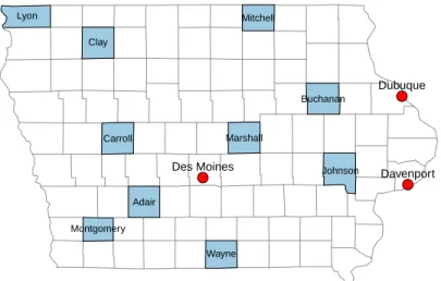
I draw my primary data for measuring intergenerational mobility in the United States early in the twentieth century from the 1915 Iowa State Census and the 1940 US Federal Census, both of which include measures of the earnings, education, and occupations of the respondents. I describe both data sources in this section, as well as the method used to link fathers in 1915 to their sons in 1940. The 1915 Iowa Census enumerated the 2.3 million Iowa residents in 1914. It was the first American census of any kind to include data on both annual income and years of education in addition to more traditional census measures, and it also includes respondent name, age, place of residence, birthplace, marital status, race, and occupation. I use the Iowa State Census sample digitised by Claudia Goldin and Lawrence Katz for their work on the historical returns to education (Goldin and Katz, 2000, 2008). The Goldin-Katz sample includes 26,768 urban residents (5.5% of the total urban population of Iowa in 1915) and 33,305 rural residents (1.8% of the total rural population). Figure 1 presents a map of the counties and cities included in the Goldin-Katz sample. The three large Iowa cities sampled are Des Moines, Davenport, and Dubuque.5 In 1915, the population of Des Moines was approximately 97,000 people, making it the 64th largest city in the country. Davenport and Dubuque were smaller, with approximately 46,000 and 39,000 people, respectively. The rural counties in the sample were selected by Goldin and Katz on the basis of both image and archive quality, as well as to provide a diverse geographic sample within the state, as shown in Figure 1.6
[Figure 1 about here.]
To construct my sample for census matching, I limit the Goldin-Katz sample to families with boys aged between 3 and 17 in 1915. These sons will be between 28 and 42 when I observe them again in 1940, which should reduce measurement issues due to life cycle variability in annual income. I restrict my analysis to sons in 1915, because name changes make it impossible to locate most daughters in the 1940 Census. This leaves me with a sample of 7,580 boys in Iowa in 1915, 6,071 of
5The census manuscripts for Sioux City, one of the other large cities in Iowa, were unreadable and not collected
by Goldin and Katz (Goldin and Katz, 2000).
whom have fathers in their households, and the requisite data on both the father’s education and income.
To locate these sons in 1940, I utilise the 100% 1940 census sample deposited by Ancestry.com with the NBER. I collect the set of possible matches, using the son’s first and last name, middle initial (when available), state of birth, and year of birth. Then, I train a record-linking algorithm and use the scores generated by that algorithm to identify the correct matches for each son from 1915 in the 1940 data.7
Once the matched sons are identified, I record the pertinent data from the 1940 census, enumer-ated in the shadow of the Great Depression and on the eve of WWII.8I use the 1940 census because it is the only census suitable for tracking the sons of Iowa. The 1940 Census was the first federal census to collect data on incomes, weeks of work, and years of education of the entire population.9
7
The machine learning approach, which I detail in Feigenbaum (2016a), teaches an algorithm how to replicate the careful hand-linking work of a researcher, but at scale and with extreme consistency. I generate the training data for the algorithm by manually linking a 30% random sample of sons from Iowa in 1915 into the 1940 census. To be considered as a possible link, records must first match exactly on state of birth, be within 3 years’ difference in year of birth, and within 0.3 Jaro-Winkler string distance in both first and last names. Then, within that filtered list of possible matches, the records are double-entry matched to the 1940 census manually by trained research assistants. Records determined to match are marked as such, records without a clear and certain match in the 1940 census are marked as unmatched. With this corpus of links, I then train a match algorithm. The match algorithm is used to reduce between-researcher variability in match quality, to speed up the matching process, and ensure data replication. The method improves on previous efforts based on phonetic matching because typos and transcription errors will not cripple the matching. The matching algorithm uses Jaro-Winkler string distances in first and last names, exact matches on state of birth, absolute difference in year of birth, Soundex matches for first and last names, middle initial matches, matching first and last letters of first and last names, and other record-based variables to predict whether a record is a true or false match. The algorithm also factors in the match quality of other possible matches for the given record searched for, only making matches when a record is a significantly better match than other possibilities. Based on cross-validated out of sample predictions within my training data, the match algorithm has a true positive rate of nearly 90% and a positive prediction rate of 86%. In Table A.3 of the appendix, I detail the exact weights on the match algorithm used.
8How might the war and Depression affect my analysis? I expect limited effects of WWII. While the war in
Europe and Asia were well underway in 1940, Pearl Harbor was still nearly two years away during the April 1940 enumeration. There was no war mobilisation in the United States in 1939 or 1940. The US spent around 2% of GDP every year on defence from 1931 to 1940, compared to 5.6% in 1941 and 16% in 1942. Spending peaked at 41% in 1945. Beyond direct defence spending, US production for the war effort is also non-existent in 1939. Cash-Carry, for example, did not begin until September 1939 (Lend-Lease in 1941) and production did not ramp up until well after the 1940 census was taken. American shipyards produced as many ships in 1941 as they had from 1938 to 1940 (Tassava, 2008). The price and wage controls (so-called ‘General Max’) were instituted during 1942, targeting March 1942 levels and suggesting that the war (or wartime policy) effects on wages or the wage distribution as of 1939 or 1940 were limited. The Great Depression’s effect is more difficult to estimate with only 10 counties and 3 cities in Iowa in my sample. Feigenbaum (2016b) shows cities with more severe Depression downturns had lower mobility, but those effects are all relative. The overall effect of the Depression on mobility is an open question.
9
The earnings in the 1940 census are top-coded at $5000. However, only 44 of the sons in my sample report such high earnings; I code them as earning $5000 for my analyses. Past federal censuses record contemporary school enrollment for each person (child), but not years of schooling completed for adults no longer in school. Earnings data was collected in 1940 only for wage and salary workers. The data collected are the ‘total amount of money wages or salary’ but enumerators were instructed: ‘Do not include the earning of businessmen, farmers, or professional persons derived from business profits, sale of corps, or fees’. For more, seehttps://usa.ipums.org/usa/voliii/inst1940. shtml#584. The importance of this missing data will vary with the fraction of farmers and other business owners in
While such data was also collected in 1950 and 1960, federal censuses are privacy-restricted for 72 year after enumeration. The data on names required for linking the 1950 census will not be accessible until 2022, 2032 for the 1960 census.10 Because it is a national sample, I do not have to worry about losing many sons to out-migration, which might otherwise bias my estimates.
My match rate is roughly 59%, which surpasses the rates of previous literature linking between censuses.11 The match rates for the rural and urban samples are comparable: I match 57.3% of sons growing up in urban areas in 1915 and 60.4% of sons from rural areas. Ultimately, I have a sample of 4,478 father-son pairs; this size is also comparable to many other projects measuring intergenerational mobility, both historically (Long and Ferrie, 2013) and recently (Lee and Solon, 2009).
1.2 What Predicts Matches?
The complexity of linking individuals between historical datasets could introduce bias to any down-stream analyses. However, I argue that my final sample does not suffer any crucial construction defects because simple transcription errors are the most likely obstacle to linking between a son observed as a child in 1915 and as an adult in 1940. To test this, I calculate a number of string- and character-based statistics using the first and last names of the sons in my sample and compare the magnitude of their effects on match rates as compared to more economically important variables.
First, I determine the name commonness of both the first and last name, relative to all names in the pooled IPUMS sample of the 1910 and 1920 censuses.12 A more common name is less likely
to have a unique match in the 1940 Census, even after limiting the possible targets by state of birth and year of birth.
Second, I calculate the length of each son’s first and last name. Longer names are more likely
my sample. It does not, however, affect farm labourers, whose earnings are reported the same as other occupations. Of my matched sample, 13.7% of the sons in 1940 are farm owners or operators without income. Initially, I drop these observations with missing earnings data in analyses on income data. However, in Appendix A.3, I impute earnings for farmers using the 1950 census, which did collect data on capital income and non-wage and salary earnings. Using these imputed earnings, I estimate even higher levels of mobility than in my main results.
10
I do make use of the 1% anonymised IPUMS sample of 1950 to impute earnings for farmers in 1940, as well as the whole sample as a check on the earnings data in 1940.
11
Parman (2011) reports match rates of nearly 50% using hand matching. Guest et al. (1989) match at 39.4%. Other attempts at census linking using phonetic codes such as Soundex have lower match rates.
12
The commonness statistic is measured as the share of 100 people in the pooled 1910 and 1920 sample with the same first (last) name. It ranges from 0.00118 (or roughly 1 person in 100,000 with the same name—these names are unique in my sample) to 1.72 for first names (John) or 1.02 for last names (Miller). Abramitzky et al. (2012) use relative commonness as a predictor of census match success as well.
to be incorrectly transcribed, but they are also more likely to be distinctive.
Third, I attempt to predict typographical errors using character similarity scores. Cognitive scientists and typographers have studied how likely certain letters are to be mistaken for one another or how similar two letters are visually. For example, readers are much more likely to mix up lower casepandqthan they would bepfork. Further, some letters are more likely to be mis-transcribed than others: sis quite visually unique whilel andn are both visually similar to other letters.13 A name with a number of l’s or n’s in it is more likely to be mis-transcribed and thus not matched when I search in the 1940 Census.14 I use a matrix of letter visual similarity from Simpson et al. (2013) to compute, for first and last names, a similarity score.15
Finally, I calculate a name’s Scrabble score as an alternative measure of both name commonness and name simplicity.16 Names with low Scrabble scores are likely to be made up of relatively common characters and are less likely to be changed or Americanised over time (Biavaschi et al., 2013).
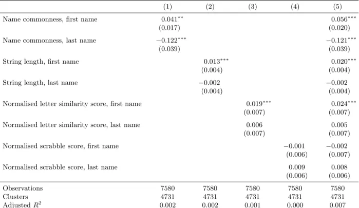
Table 1 presents the results from a series of linear probability models, predicting whether or not a son in 1915 is uniquely matched ahead to the 1940 Federal Census. Sons with more common last names are less likely to be matched, while first name commonness has a smaller, positive effect. Sons with longer first names or first names with higher similarity scores are more likely to be found, but both of these effects are quite small.17 The overall explanatory power of these variables in Table 1 is quite low; however, I argue that this underscores the randomness with which some sons are linked and others are not. Mismatches are driven by transcription errors (both by census enumerators and in contemporary data entry) which are largely random, even if some predictors (common names, letter similarity) have some power. I include controls for all of these name string
13lis likely to be confused withf andifor example, whilenis similar to bothhandm. 14
Recall matches are made using census indices transcribed by Ancestry.com.
15
Specifically, Simpson et al. (2013) conduct surveys of college students and other native and non-native English readers to assess the similarity of letters on a 7 point scale, where 7 indicates exactly the same and 1 extremely different. For example,iandlhave a similarity score of 6.13, whilewandthave a similarity score of exactly 1. I take the highest (non-self) similarity score for each letter as a measure of a letter’s likelihood of being mis-transcribed. Figure A.1 in the appendix graphs these scores for each letter. Then, I calculate the average of these scores for all letters in a given string (name). The scores from Simpsonet al are based on both lower case and upper case letters in block type. As many of the census files are in script, a visual similarity matrix for cursive letters would be ideal, but such a measure does not exist in the typography literature. As a robustness check, I also use a letter matrix of confusion probability from McGraw et al. (1994) and find a high correlation between each letter’s similarity score.
16
Biavaschi et al. (2013) introduce the use of Scrabble scores into the economic literature. They use this measure to predict name changes by immigrants to the United States during the early twentieth century. Scrabble point values were based, originally, on the frequency of letters on US newspaper front pages.
properties in all subsequent analysis.
[Table 1 about here.]
More serious issues could be generated by differential matching rates according to father, son, or family characteristics in 1915. In my sample I find little evidence that such characteristics strongly affect the probability of matching. In Table 2, I present the estimated effects of a set of variables observed for fathers and sons in 1915 on the probability of positively locating the son in the 1940 Census.18 Each row in the table is a separate linear probability regression, reporting the coefficient of the listed X variable while controlling for first and last name commonness, length, letter similarity, and Scrabble score. I am slightly more likely to match sons who had higher income or more educated fathers (or mothers) in 1915, but these effects are both economically and statistically insignificant. For example, the probability of matching a son with a father at the 25th percentile of income is only 1 percentage point lower than matching a son with a father at the 75th percentile of income. Similarly small effects of both father’s and mother’s education can be seen as well. I am also less likely to match sons in the urban sample which follows from the slightly higher match rate among rural sons. I am also more likely to link sons born in Iowa, even after conditioning on name string characteristics.19 All analysis undertaken in this paper will include controls for son’s place of birth, place of residence in 1915, and, where appropriate, father’s place of birth.
[Table 2 about here.]
1.3 How Does Iowa 1915 Compare to the US in 1915?
Iowa undertook an enumeration of its population in 1915 unlike any other in American history. In addition to gathering reliable ‘characteristics of population [and] agricultural and other industries’, the census also collected data on the earnings of its citizens and the extent of education in popula-tion. The census report announced that the finding ‘happily confirms the claim of very high rank
18Results in this matching exercise are robust to alternative regression models, including logit and probit models.
I use a simple linear probability model for ease of interpretation.
1986% of the sons in my sample were born in Iowa so there is no difference between the 25th to 75th percentile for
for Iowa in educational standing’.20 That Iowa collected such earnings and education data makes the present study possible, but its rarity among contemporary censuses also raises a question: how unique was Iowa and how might that affect my estimated mobility rates?
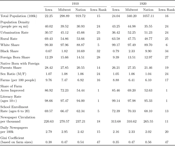
How does my sample compare to the rest of the US in 1915? To be certain, the father and son pairs in my linked sample are not a random of the nation in 1915 and Iowa is not the median state. In Table 3, I compare Iowa to the rest of the nation and the Midwest in both 1910 and 1920 on a variety of dimensions.21 In some ways, Iowa is a representative state: it is ranked in the middle of
the United States in population density, urbanisation, and rural share, as well as sex ratio. Iowa was a more agricultural economy than the nation, but still one-third of states had more farms per capita.
However, the racial make-up of Iowa, its education, and inequality are outliers. The state was more than 99% white in both 1910 and 1920, even a few points whiter than the rest of the Midwest. Only 12% of the Iowa population was foreign born in 1910 (falling to 9% in 1920), lower than the national rate, but only slightly behind the median state. That contrasts with the prevalence of second-generation immigrants in Iowa: 28% of Iowa were the native born but to foreign parents in 1910, 8 points higher than the national rate.22 Iowa’s commitment to education—it was a leading state in the high school movement (Goldin and Katz, 2011)—is also apparent in Table 3. Iowa led the nation in 1910 and 1920 in literacy and was highly ranked in school enrollment as well. Goldin and Katz (2000) document the high returns to education in Iowa in 1915, both among white-collar and blue-collar workers Iowa was also above the median in newspaper circulation and number of newspapers (Gentzkow et al., 2011). Finally, when I calculate inequality using the distribution of farm sizes in the census, Iowa is the second most equal state in the continental US in both 1910 and 1920.
[Table 3 about here.]
How might the differences between Iowa in 1915 and the rest of the nation affect my analysis?23
20
Preface to the Iowa 1915 Census Report, page iii. Given that Iowa was the first and only state to collect data on educational attainment, it is unclear how such a rank was calculated, but the fact that such data was even collected points to Iowa’s standing.
21I include the states of Illinois, Indiana, Michigan, Ohio, Wisconsin, Iowa, Kansas, Minnesota, Missouri, Nebraska,
North Dakota and South Dakota in the Midwest.
22
I aggregate the census totals for native born with two foreign parents and native born with one foreign parent.
Iowa’s racial homogeneity may create more mobility than in the rest of the country. If the Gatsby Curve—as Krueger (2012) dubbed the correlation in OECD countries in the last decade between intergenerational mobility and inequality—held in the early twentieth century, again, perhaps Iowa will demonstrate more mobility than other states in this era because of its low inequality levels. Alternatively, the relatively low share of the foreign born may reduce mobility, if the children of recent immigrants are likely to experience fast upward mobility as they assimilate. In the analysis that follows, I take Iowa’s uniqueness into account when comparing mobility over time and attempt to contrast my findings not with mobility overall but with contemporary estimates of mobility in an Iowa-like sample.
In the appendix, I present summary statistics on the men in my linked sample, exploring how the fathers and the sons in the sample differ from the matched fathers and sons. The first two columns of Table A.1 present summary statistics for the fathers of children between 3 and 17 in the Goldin-Katz Iowa State Census sample. Fathers found are the fathers for whom sons were located in the 1940 Census through Ancestry.com. Average yearly earnings for the fathers are approximately $1000 in 1915 dollars. The average father had a half year more than a common school education (eight years) and was approximately 42 years old in 1915. Of the fathers in my sample, those fathers for whom I matched a son into the 1940 Census earned very slightly more, though not significantly so, measured either in levels, logs, and weekly earnings. The final two columns of Table A.1 present summary statistics for the Iowa sons in my sample. Only summary data for sons with complete information in the 1940 Federal Census is reported in the table, which lowers the number of observations in the final column to 3,971. The located sons earned more than $1400 in 1940, which is roughly the same in real terms as the average earnings for their fathers in 1915; the lingering effects of the Great Depression may have reduced any real income gains overall.24 Also notable is the fact that the sons had on average two more years of schooling than their fathers.
enter WWI until April 1917 and the draft did not begin until May 1917. Fighting in Europe began in July 1914, but little if any economic effects of the first six months of the war would have been felt by the residents of Iowa. Rockoff (2008) documents no rise in the industrial production or the stock market in response to the beginning months of European fighting. Changes in taxing, spending, and borrowing, particularly the famous liberty bond programme, were not introduced until October 1917. None of the fathers in my sample had been mobilised and any fathers working in industries that might later be subject to government price or wage controls were not subject to them in 1914. In the nearly 800 page report on the 1915 Iowa Census, published in 1916 by the enumerators, the ongoing European war was not mentioned.
24
I measure all dollar amounts in this paper in nominal terms. Because I use logged earnings in my regressions and income for all sons is measured in 1940 and for all fathers in 1915, any nominal to real conversions drop out into the unreported constant term.
This is a striking example of the effect of the high school movement and the expansion of public education in Iowa, previously documented by Goldin and Katz (2008) and Parman (2011).
2
Measures of Intergenerational Mobility
The measure of intergenerational mobility is often constrained and influenced by the information available in linked intergenerational samples, both historically and in contemporary data. In this paper, because I observe earnings, occupations, education, as well as names, of the fathers and sons from Iowa 1915, I calculate a variety of different mobility measurements on a consistent dataset and am able to establish whether or not the measures produce similar results. In this section, I describe the various measures I am able to consider.25
2.1 Intergenerational Income Mobility
The most common measure of intergenerational economic mobility is the intergenerational elasticity of income (IGE), estimated by regressing the son’s log income against his father’s log income. Corak (2006), Solon (1999), and Black and Devereux (2011) present thorough reviews of the IGE literature.26 These reviews all indicate a lack of historical data on intergenerational mobility: Corak (2006) documents 41 studies of the US IGE, none of which presents data before 1980. One aim of my project is to establish a correct measure of IGE well before the period previously studied in this literature.27
Corak’s preferred measure of IGE in the US is 0.47, in line with the reviews presented by both Solon and Black and Devereaux.28 Hertz (2009), who is able to split the sample by race, estimates
25One major limitation imposed by my data is that I am unable to estimate wealth mobility. Often drawn from
probate records (Clark and Cummins, 2015), American federal censuses recorded data on wealth only three times (1850, 1860, and 1870). Ager et al. (2016), looking in the postbellum South, find high rates of mobility of wealth, in agreement with the findings I present later in this paper.
26The estimated elasticity of income between one generation and the next is commonly referred to as an IGE and
I will use that abbreviation here.
27Aaronson and Mazumder (2008) take a different tack when measuring intergenerational income mobility. They
use successive waves of the US federal census, from 1940 to 2000, and construct synthetic parents for observed individuals. They find low levels of mobility in 1940, but more mobility each decade until 1980. Mobility falls again in 1990 and 2000. However, the parents are constructed only using state of birth, age, and race; thus rather than regressing the son’s income on the father’s, they regress the son’s income on the average income of men of the same race in the son’s state of birth. While that is a possible proxy for the father’s income, it does not seem sufficiently detailed or granular to detect small shifts in the intergenerational transmission of income.
28Corak also gives lower and upper bounds of between 0.40 and 0.52. Mazumder (2015) argues for a parameter of
an IGE of between 0.39 and 0.44 for whites, the relevant comparison here given the high white share in my Iowa sample. Corak (2006) also documents large variations between US studies measuring the intergenerational elasticity of income.29
However, the IGE imposes a very particular functional form relationship between the son’s and father’s earnings.30 Chetty et al. (2014a) present evidence from recent US tax data that suggests this assumption is false; Corak and Heisz (1999) show the same with Canadian tax data. At both tails of the income distribution, the linear relationship between the father’s log income and the son’s log income breaks down. Following Dahl and DeLeire (2008), Chetty et al. (2014a) and Chetty et al. (2014b) estimate a rank-rank parameter of intergenerational mobility, regressing the son’s income percentile (within his cohort) against the father’s income percentile (within his cohort). The graphical evidence presented in Chetty et al. (2014a) suggests that the implied linearity in the rank-rank specification is a more accurate fit of the data. For their sample of the US, Chetty et al. (2014a) estimate a rank-rank parameter of 0.341 overall and 0.336 for sons. However, similar to the IGE literature, there are few historical estimates of the rank-rank parameter: Chetty et al. (2014b) plot trends in mobility for sons born between 1971 and 1993, but they cannot extend their sample further back in time.
I am able to estimate both IGE and rank-rank mobility in my data because I observe earnings for fathers in Iowa in 1915 and earnings for their sons in the 1940 Federal Census.
My study is not the first to use the earnings data in the Iowa 1915 census to estimate inter-generational mobility in the early twentieth century. Parman (2011) uses a clever multiple match technique to create father-son links within the Iowa 1915 census, even though the adult men in
29See, for example, the first table in Corak’s appendix. IGE estimates in the literature range from 0.09 to 0.61.
Because of this variation scholars have focused on measuring changes over time in IGE within one consistent dataset. However, the results in this literature have also been rather inconsistent. Mayer and Lopoo (2005) use the PSID and collect a sample of 30 year olds, regressing the son’s income at age 30 on a three year average of the father’s income. They find a large and statistically significant downward trend in the IGE, suggesting that mobility has increased significantly in the last several decades. Levine and Mazumder (2002) present more mixed results in work using the NLS, GSS, and PSID. Levine and Mazumder observe sons between the ages of 28 and 36 in 1980 and again in 1990. They find increasing mobility in the PSID, but decreasing mobility in the NLS and GSS. Lee and Solon (2009) argue that past work has been plagued by non-classical measurement error. To correct this, they argue that rather than observing the son’s outcomes once or twice and throwing away the rest of the data, researchers should make use of the full sample. Drawing on PSID data for cohorts of sons and daughters born between 1952 and 1975, Lee and Solon do just that. I focus on the Lee and Solon results for fathers and sons to keep in line with the analysis I am able to perform in my data. Controlling for a quartic in the ages of both parents and children, they only limit the sample to sons between 25 and 48. They find a simple average IGE of 0.44 over the period and no statistically significant trends in IGE between 1976 and 2000.
30
the Iowa sample are no longer in their parent’s households. Parman matches the men backwards in time to the 1900 Federal Census to construct childhood households. Though most are heads of household in 1915, these are Parman’s ‘sons’ in the analysis. The reconstructed households yield the name, state of birth, and other demographic characteristics of the ‘fathers’ in 1900. Parman then matches these fathers forward in time to the 1915 sample, thus observing both fathers and sons in Iowa in 1915 and estimating IGEs based on income reported in the Iowa State Census. Parman finds an IGE of approximately 0.11 for all father-son pairs or 0.17 for non-farmer father-son pairs. These low estimates paint a picture of high levels of mobility in the early twentieth century.31
Parman finds very low rates of persistence in status. However, his analysis is limited in two key ways by the data available to him when he undertook his study.32
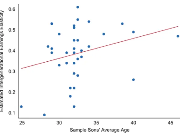
First, his sample was made up of very old fathers and very young sons. The average age of fathers in Parman’s sample is between 57 and 65, depending on the particular specification. This age range is on the far right tail of the IGE studies in the literature and thus is very likely to present a very low IGE, due to life-cycle-induced measurement errors. The average age of the sons in Parman’s sample is between 25 and 30, and this may also bias his results towards a very low IGE. As Grawe (2006) and Haider and Solon (2006) describe, trends in life cycle earnings—particularly, the fact that people with higher permanent income experience more earnings growth earlier in their career—can bias the estimate of β (Mazumder, 2015). Empirically, the sample age bias can be seen in Figure 2, based on the American IGE literature surveyed by Corak (2006). As the first figure shows, the older the average age of the fathers in the study samples, the lower the estimated intergenerational elasticity. The second figure shows a similar but weaker relationship holding in the opposite direction between estimated IGEs and the average age of sons in the sample.33 Because Parman measured both fathers’ and sons’ earnings in the 1915 census, his sample was necessarily made up of fathers later in the life cycle and sons early in theirs. With the recent availability of the 1940 Federal Census, I am able to draw my sample from a set of fathers and sons with average ages of 40 and 35.
31
These estimates are similar but much lower than the income IGE estimates I will present later in this paper.
32Full access to the 1940 Federal Census, including all citizens’ names, was not available until April 2012, well after
Parman completed his research.
33Both of these best fit lines are statistically significant in the univariate regression, but the relationship between
father’s age and estimated IGE is much stronger. The points graphed in Figure 2b suggest instead that with sons ages ranging from approximately 30 to 35, the estimated IGE should not be a function of the data sample.
[Figure 2 about here.]
The second data-driven limitation is that the Parman (2011) sample is restricted to fathers and sons both living as adults in Iowa in 1915 because the 1940 Federal Census was not available until 2012. How large is the bias of this restriction, and in what direction does it push the intergenera-tional income mobility results? In the results section that follows, I will be able to use my sample to better understand the magnitude and direction of the problem by limiting my sample to only those sons who still live in Iowa in 1940. To preview, I find that the bias is large and negative: selecting the sample using only sons remaining in Iowa in adulthood reduces both the measured IGE and rank-rank parameters.34 Because the state of residence in adulthood is, in part, jointly determined with the outcome of interest (earnings), controlling for it or splitting the sample based on it is problematic. In order to estimate an accurate IGE parameter for the early twentieth century, one needs to be able to observe sons that remain in their father’s state of residence and sons that move elsewhere.35
Thus, while the results in Parman (2011) suggest that income IGE was very low and that income mobility was very high in Iowa in 1915, data constraints complicate the comparison of the estimated IGE to other time periods and places.
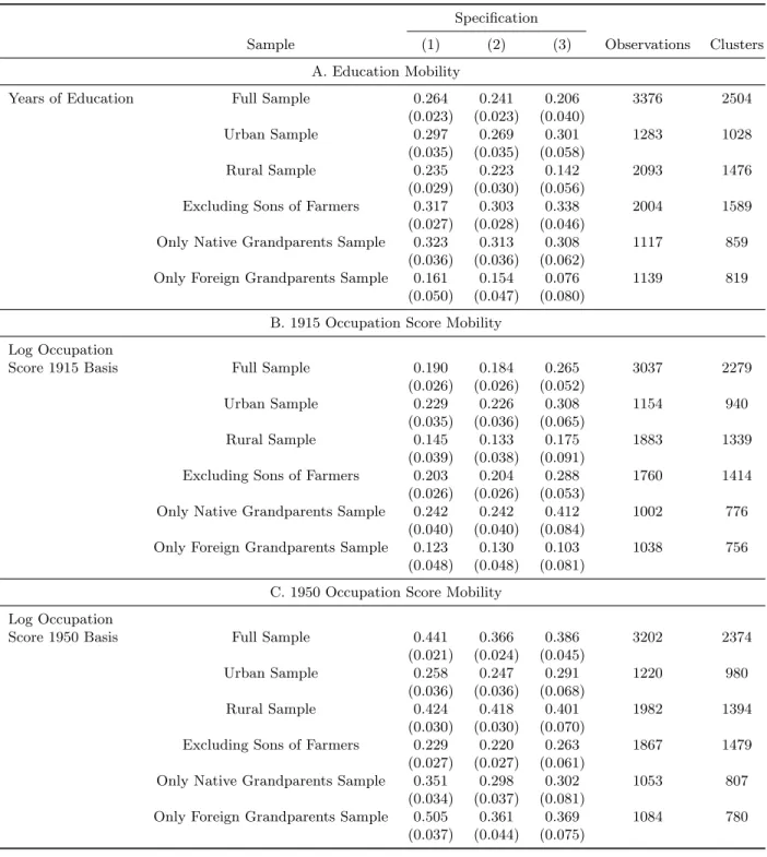
2.2 Intergenerational Education Mobility
Due to data constraints, there has been little work on educational mobility in the US historically.36
Hertz et al. (2007) present the most comprehensive measures of intergenerational elasticity of education across many different countries and regions. They find an IGE of education for the US of 0.46, suggesting more mobility of education in the US than in South America (0.60) but less than in Western Europe (0.40).37 With data collected on years of education in 1915 in Iowa and in 1940 nationally, I am able to construct the earliest educational mobility estimates for the United States.
34
These findings are in the final rows of both panels A and B in Table 4.
35
My sample is technically restricted to those sons still living in the US and enumerated in the Federal Census. However, the number of sons moving abroad in this period is likely very low and thus the bias is likely to be insignificant.
36Parman (2011) measures the effects of public education on income mobility, but does not estimate father to son
educational mobility directly. Outside of the US, Checchi et al. (2013) study Italian cohorts born between 1910 and 1970 and find very high IGEs and low mobility of education in their early samples, relative to the recent period.
37
The use of the IGE term and elasticity more generally is a bit of an abuse of notation. The IGE literature on education estimates these parameters using levels on levels, rather than log on log.
In addition, because education is significantly less noisy as a proxy for status than a single year of earnings, the educational mobility results can serve as a check on mobility based on earnings, which may be biased down due to noise.38
2.3 Intergenerational Occupational Mobility
The study of historical intergenerational mobility has focused on the study of occupational mobility because occupational data has historically been much more available. Early work on this topic was undertaken by Thernstrom (1964, 1973), studying the occupations of successive generations in Boston and Newburyport, MA. Thernstrom tends to find quite high upward mobility, but a lot of white collar stability as well. Duncan (1965) finds more upward and less downward mobility in 1962 relative to the occupational transition matrices of 1952, 1942, or 1932, relying on data gathered from Occupational Changes in a Generation (OCG). However, neither Duncan nor any of the subsequent work based entirely on the OCG data is able to measure occupational mobility for earlier periods.
Guest et al. (1989) compare a nineteenth-century sample, built by matching fathers and sons in the 1880 to 1900 censuses, to the OCG. They find less upward mobility and more occupational inheritance in the nineteenth century. However, for fathers and sons who are not farmers, the association is both economically smaller and statistically weaker. The results depend a great deal on where Guest et al. put farmers in the occupational distribution.
To avoid the fraught issue of how to rank occupations—especially without available average income, education, or wealth data by occupation—the economics literature has turned to occu-pational transition matrices, which are agnostic about movements up or down the occuoccu-pational ladder and instead focus only on movements by the son out of the father’s occupational category. In particular, Altham and Ferrie (2007) present the Altham statistic, which has become the stan-dard measure of intergenerational occupational mobility in economics. To compute these measures of occupational mobility, fathers and sons are each grouped by occupation into one of four broad categories—farmer, white collar, skilled and semi-skilled labour, and unskilled labour—within an occupation transition matrix. The Altham statistic measures the strength of association between
38In my sample, it is very unlikely that any of the fathers or sons continued education beyond when I observe them
both the rows and columns of a transition matrix and between any two matrices. Altham statistics can be defined for any two matrices. Specifically, let bothP and Qber×smatrices with elements pij andqij. Then the Altham statistic is:
d(P, Q) = r X i=1 s X j=1 r X l=1 s X m=1
log pijplmqimqlj
pimpljqijqlm ! 2 1/2 (1)
Altham and Ferrie (2007) use thed(P, Q) notation to convey the sense in which the Altham statistics are distance measures.39 d(P, I), where I is the occupation transition matrix of perfect mobility (that is, a matrix with ones in all rows and columns), can be used as a measure of distance from independence.
One of the strongest criticisms of using occupations to study long-term trends in intergenera-tional mobility is the difficulty in classifying farmers (Xie and Killewald, 2013).40 Comparison of mobility measures across time is complicated—perhaps even driven—by the movement out of agri-culture in the US. For example, Guest et al. (1989) conclude that there was more social mobility in the post-WWII period in the US than there had been in the nineteenth century, but they suggest that this reflects the high-heritability of farming and the declining shares of farmers since the late nineteenth century. In this paper, I attempt to control for that by comparing relatively homoge-neous samples over time, particularly by constructing a sample in the PSID or other contemporary data that is as rural, white, and agricultural as my Iowa sample. I also focus more analysis on the urban Iowa sons, almost none of whom had farmers for fathers or became farmers themselves.
The second problem posed by farmers is their extreme distribution of earnings. In the standard census sources, including both the 1915 Iowa State Census and the 1940 Federal Census, an indi-vidual classified as a farmer may be a small-scale tenant farmer, renting his land and equipment and working a small plot. However, owners of very large farms are also classified simply as farm-ers. It is quite possible for a father and son who are both farmers to have very different incomes. Similarly, a shift between a father and son from farming to another occupational category may represent an increase or a decrease in income. Further, to what extent is the wide variation in
39As a distance measure, Altham statistics satisfy the triangle inequality. For any threer×smatricesA, B, C, it
is true thatd(A, C)≤d(A, B) +d(B, C).
40Income measures for farmers, when available, are not a panacea either. To the extent farmers are engaged in
income among farmers driven by measurement error or transitory income shocks (annual weather shocks, for example)?
When considering an intergenerational sample drawn from a population with a large share of farmers, measures of income mobility and occupational mobility may diverge. In this paper, I measure both income and occupational mobility, as well as educational mobility, for such a population.
2.4 Name-Based Intergenerational Mobility
Both given names and surnames contain socio-economic data. Recent research has utilised this to estimate intergenerational mobility, either as a complement to exact parent-to-child links or a substitute when such links are not possible.
Olivetti and Paserman (2015) create pseudo-links using the content of first names. If families of different means or status have different naming patterns, then even after a child leaves his or her parent’s household, the child’s name carries with it a proxy for his or her parent’s outcomes. For any given name in the population in one census, they calculate the average occupational status (using occupation scores, as described above) of fathers with children of that name. Then, in a later census containing the adult selves of the children in the previous step, they relate the outcomes of the second generation to the implied status of their (unobserved) parents based on their names. Olivetti and Paserman (2015) document decreases from 1870 to 1940 in mobility, consistent with the trends in Long and Ferrie (2007). Because I am working with historical data that includes names of both generations, I am able to implement these name-based mobility measures as a complement to estimates based on my linked sample.
Surnames also convey information about the previous generation. In recent research, Greg Clark and coauthors use rare last names to measure mobility, both between parents and children (Clark and Cummins, 2015), as well as in the very long run (Clark, 2014). Guell et al. (2015) formalise such a method of measuring mobility based on surnames and show declining mobility in Catalonia over the century. One major advance with the rare surname method is its flexibility: whether based on admissions lists from elite academic institutions or probate records or voting records, any data containing both last names and a measure of status can be used to estimate mobility. Clark (2014) argues that these measures tend to suggest far less mobility than one generation
income or occupational status mobility measures. Studying mobility based on the over- or under-representation among doctors or lawyers of historically prestigious surnames in the United States, Clark et al. (2012) find advantages persisting for at least 5 generations. While my two generation sample does not permit such long run estimates of mobility, I am able to apply Clark’s method to the sons of Iowa to estimate the changing shares of elite surnames in certain occupations, focusing on doctors and lawyers as in Clark et al. (2012).41
3
Intergenerational Mobility Estimates for Iowa from 1915 to 1940
How much intergenerational mobility was there in Iowa in the early twentieth century? How do the measures of mobility reviewed in the previous section compare? When data constrains researchers from studying one or more of these measures, are the other measures plausible substitutes? In this section, I estimate the intergenerational mobility of income, earnings rank, education, and occupation, as well as mobility measures based on the socio-economic content of names. I document that these measures are all in general concordance with one another in my sample in two ways. First, all measures suggest that early twentieth-century Iowa was a place of high intergenerational mobility. Second, the relative rates of mobility between urban and rural sons, as well as between sons with native-born versus foreign grandparents, are all roughly consistent across measures. I also argue that, based on a variety of measures, there was likely more mobility in Iowa historically than there is today.
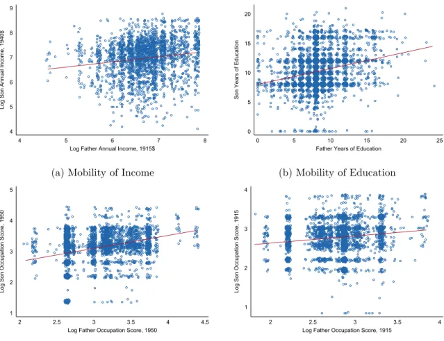
I begin by presenting raw intergenerational correlations of fathers’ and sons’ outcomes in Fig-ure 3: log annual income (3a), years of education (3b), and occupation score based on 1950 scores (3c) and on 1915 scores (3d).42 The intergenerational correlation is one possible measure of mobil-ity and holds trends in the marginal distributions—the dispersion of earnings among fathers and among sons—fixed. In log earnings, the correlation is 0.14; the education correlation is a bit higher (0.24).43 Clearly, there is a strong positive relationship between outcomes for fathers in 1915 and
41Guell et al. (2015) develop an alternative metric for deriving the informational content of surnames. 42
Naturally, there are many father-son pairs with the same outcome levels as other pairs. In an attempt to display this density at certain points on the graphs, I have used both hollow scatterplot markers and jittered the data. The best fit lines are, of course, drawn based on the full sample before jittering. The $5000 top coding in the 1940 census is apparent on the right side of Figure 3a.
43
The occupation-based measures differ, depending on the year used to construct occupation scores. The 0.14 correlation coefficient based on 1915 scores suggests a lot of mobility, while the 0.36 estimate based on 1950 scores does not.
sons in 1940 but the exact measure of the respective slopes of these lines—and how those slopes compare across the various measures of mobility, as well as with the estimates of mobility in the recent period—is the key question of this paper.
[Figure 3 about here.]
3.1 Intergenerational Mobility of Earnings
I measure mobility of earnings in two primary ways. First, following the intergenerational mobility literature, I use intergenerational elasticities (IGE) (Corak, 2006; Solon, 1999; Black and Devereux, 2011). The canonical formulation regresses the son’s adult outcome, in my case as measured in the 1940 Census, on the father’s adult outcome, as measured in the 1915 Census. Let Yi be the outcome of interest, either (log) income or education. The model I estimate can be summarised as:
Yi,s1940 =α+β·Yi,f1915+Qs(agesi,1915) +Qf(agefi,1915) +Qs(agei,s1915)×Yi,f1915+i (2) β can be thought of as a persistence parameter: larger estimates mean a tighter link between father and son and thus less mobility.
Second, following Dahl and DeLeire (2008) and Chetty et al. (2014b,a), I also use rank-rank estimates. Again, I regress the son’s outcomes on the father’s outcomes, but where outcomes are the relative positions or percentiles in the income distribution. For sons observed in 1940 I use the full 1940 IPUMS census sample to calculate the full income distribution of white men, aged 28-42, matching the demographics of my sample. For fathers, income data are not available for a nationally representative sample. I instead calculate the full income distribution of white men in the Goldin-Katz Iowa 1915 census sample with the same age range as the fathers in my sample. Ranks are scaled as percentiles between 0 and 1; a rank of 0.5 indicates that the father or son is at the median for annual income.
To reduce any measurement error induced by life cycle income effects (Grawe, 2006), I follow Lee and Solon (2009) and include quartic age controls for both the father and the son, defined as Qs and Qf above, as well as an interaction between the son’s age and the father’s outcome. In the interaction term, I normalise son’s age in 1940 relative to age 40 (Haider and Solon, 2006).44
44
The fact that I define my sample to observe sons between ages 28 and 42 in the 1940 Census also reduces life cycle driven measurement error. As some of my observed sons are brothers, I cluster standard errors at the family level. I also include an Iowa 1915 county fixed effect, subsuming an urban or rural control. The results are robust to the inclusion of controls for family-size effects, county fixed effects, and the name string control variables described previously.45
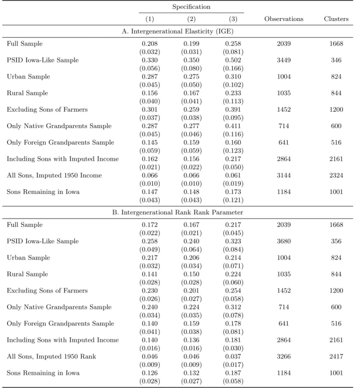
Panel A of Table 4 presents my estimates of the IGE of income across a variety of samples. Both the father’s and son’s incomes are measured as annual log earnings.46 The first specification is a
simple univariate regression of the son’s log earnings on the father’s log earnings. In specification two, I include controls for name string properties that might affect matching, 1915 county of residence fixed effects, and quartic controls in father and son age. In the third specification, I also include an interaction between son’s normalised age and father’s log earnings to control for life cycle measurement error (Grawe, 2006; Haider and Solon, 2006).
My baseline estimates for the IGE parameter for the full sample of Iowa fathers and sons range from 0.199 to 0.258, as shown in the first row of Table 4. The literature suggests an IGE of 0.47 for income in the United States today (Corak, 2006). Lee and Solon (2009) argue that the IGE of income has been roughly stable for cohorts observed between the late 1970s and the early 2000s. My results suggest that this recent stability does not extend historically, and that there was much more intergenerational mobility of income in the early twentieth-century US than there is today.47
the son is age 40. I follow Lee and Solon (2009) in normalising to 40.
45The county fixed effects indicate the county of residence when the son is observed in Iowa in 1915. The name
string controls include first and last name commonness, length, letter similarity, and Scrabble scores, all attempts to control for differential matching rates between the 1915 and 1940 censuses. While I include these various controls to reduce measurement error, both Chetty et al. (2014a) and Nybom and Stuhler (2014a) present extensive results that suggest the rank-rank measures of intergenerational mobility are much less susceptible to biases. Working with the universe of US tax records, Chetty et al. (2014a) argue that estimates are stable even with just one year of income observed for both fathers and sons, though this is still an unresolved issue in the literature. Further, they document that the exact age when fathers or sons are observed has very little effect on the measurement of mobility, so long as the fathers are observed between the ages of 30 and 55 and the sons are observed after age 30. Nybom and Stuhler (2014a) replicate these lessons for the estimation of rank-rank mobility using Swedish data. The stability of my estimates of rank-rank mobility with and without various controls suggests that the rank-rank parameter is quite robust in my historical sample as well.
46To ensure comparability with contemporary estimates, I use annual earnings, not weekly earnings. Results using
weekly earnings are similar and in fact lower than those presented in Table 4, suggesting even more mobility in the early twentieth century.
47
One concern with the results presented thus far is the reliance on the log transformations of the income data. By logging income, the assumption made is that small changes in income for very poor fathers have much higher returns (to the son’s income) than smaller changes further up the income distribution. In the appendix, I show that these results are robust to alternative transformations of the father’s and son’s income variables, including both levels and square roots.
[Table 4 about here.]
Similar to my IGE results, I find much more income mobility historically than today. The rank-rank parameter ranges from 0.167 to 0.217 in the first row of Panel B of Table 4, the main sample with all linked father-son pairs. Chetty et al. (2014a) measure a rank-rank parameter of 0.341; among just male children, they find a rank-rank estimate between 0.307 and 0.317.
However, any measurement error will tend to bias down estimates of intergenerational mobility (Solon, 1999). Further, though Iowa is in some ways broadly representative of the US in 1915—with respect to urban and rural shares—the differences in my estimated mobility may reflect differences between Iowa and the rest of the country, not differences between time periods. In fact, according to contemporary data, children born in Iowa are among the most economically mobile in the entire country, across many measures (Chetty et al., 2013).
I attempt to standardise my comparisons in two ways. First, I construct a sample of recent intergenerational data that is demographically comparable to my Iowa sample, drawing on data from the PSID. To do this, I limit the PSID to include only white father-sons pairs (99% of my linked Iowa sample is white). I also limit the PSID to sons who grew up in the Midwest.48 The
results are presented in the second rows of each panel in Table 4 (Panel A for IGE, Panel B for rank-rank).
To calculate a comparable contemporary IGE, rather than follow Lee and Solon (2009) and measure the father’s income as the average of his income when the matched son is between 15 and 17 years old, I use the father’s income when his son is 10.49 In doing so, I attempt to replicate the noise in my historical data from only observing income once. The son’s income is observed in each year that the son is in the PSID and is between the ages of 28 and 42, to match my 1940 census data. Both income variables are measured in 2000$.50 Limiting the PSID to sons born in
the Midwest, I estimate an IGE between 0.33 and 0.50, depending on the use of state fixed effects
48
The Midwest region is defined in the PSID as Illinois, Indiana, Iowa, Kansas, Michigan, Minnesota, Missouri, Nebraska, North Dakota, Ohio, and South Dakota. I do not limit the PSID sample just to sons raised in Iowa as there are only 385 father-son pairs with the requisite data.
49Mazumder (2009) underlines the downward bias on mobility estimates when using only a single-year of earnings
data. I cannot create additional years in my historical data, but I can ensure the contemporary comparison is afflicted by the same potential single-year bias as my Iowa data. I use 10 because this is the midpoint of my age range for sons in the 1915 sample. If I do not observe a father in the year when his son is 10, I use the year when the son is closest to 10 in the PSID sample.
50
While I attempt to match my age and county fixed effects from my Iowa sample results with age quartics and ‘grew up’ fixed effects, I do not observe either family size or name strings in the PSID.
and age controls.51 Though the Iowa-like samples in the PSID are small and contain repeated observations of the same set of father-son pairs over many years, the results suggest that the lower mobility I find historically is driven neither by the demographic composition of my data nor by the single-year measurements of income. I come to a similar conclusion when comparing my estimates of rank-rank mobility with contemporary measures. The first comparison, shown in the second row of Panel B of Table 4, is the rank-rank mobility using the PSID sample. For the Midwest sample, I measure a lower parameter than is found nationally, suggesting the Midwest is more mobile; however, these estimates are far larger than what I find historically in the full sample.
As a second alternative construction of comparable recent mobility parameters, I use the county level results reported by Chetty et al. (2014a). Unfortunately, such a comparison can only be made for the rank-rank parameter, as Chetty et al. (2014a) do not calculate IGE at any disaggregated geographies.52 When I calculate the weighted average of rank-rank mobility, weighing by the shares of my sample living in each county in 1915, I find a rank-rank parameter of 0.303, similar to the result from the contemporary PSID data and, more importantly, far larger than the rank-rank parameter of 0.169 to 0.219 that I find in my historical sample.53
In the appendix, I show that neither false matches in my census linking procedure nor higher levels of measurement error in historical data could account for my estimates of lower IGE param-eters (and thus higher mobility) in the 1915 to 1940 sample relative in the contemporary sample. Via simulation, I introduce both mismatches and measurement error into my Iowa-like PSID sam-ple considered above. The share of false matches would have to approach 50% for mismatching to account for the estimated differences in IGE parameters, which seems highly unlikely.54 As detailed in the data section, the matches were carefully constructed based on first and last names, year of birth, state of birth, and gender. In addition, the measurement error simulations suggest that earnings measures from the 1915 and 1940 censuses would have to be considerably noisier than
51
Specification 3 includes interactions with father’s outcomes and son’s ages. However, the PSID includes a small number of father-son pairs observed repeatedly which may complicate the interpretation of this estimate. Specification 1 and 2 are preferred and more conservative as comparisons.
52Hertz (2009) does calculate mobility rates by race; given the very high white share in Iowa in 1915, his estimates
of 0.39 or 0.44, depending on the adult equivalent adjustments in each specification, are similarly indicative of reduced mobility in the present period relative to 1915 Iowa.
53
I can also split the sample between the urban and rural counties in my analysis. The weighted average of rank-rank mobility is 0.355 in the three urban counties and 0.268 in the 10 rural counties.
54
That is, 50% of sons that I find in the 1940 census and link back to 1915 on the basis of the son’s first and last names, state of birth, and year of birth would have to be the wrong person. For the rank-rank parameter, the mismatch error required to shrink the difference between the estimates is roughly 30%.
earnings measured in the recent period to generate the large difference in IGEs.
Are the high rates of mobility that I find driven by the movement off the farm in the early twentieth century?55 To answer this question, I compare differential mobility for both sons of rural and urban Iowa, splitting the sample according to where the sons were living when their fathers were first sampled in the 1915 Iowa State Census.56 The results for these subsample analyses are presented in the third and fourth rows of Table 4. Only 18 of the urban sons have a father farmer in 1915 and only 60 are farmers in 1940. Sons observed in rural Iowa in 1915 are more mobile than their urban peers as measured both by IGE and rank-rank parameters, though the differences are not statistically significant for the rank-rank mobility estimate. All measures still show more mobility historically than is estimated in today. The much higher levels of mobility for rural sons may be driven by the large increases in access to public education even in remote, rural regions of Iowa (Parman, 2011). Alternatively, the high levels of mobility may be caused in part by movement off the farm; this finding is consistent with the model of human capital transmission presented by Nybom and Stuhler (2014b), which suggests that periods of structural transformation in the economy weaken the links between parents’ and children’s outcomes.
Further isolating the effects on mobility of the shift away from agriculture, I limit the samples in the fifth rows of both panels A and B to only sons with fathers who were not farmers.57 Again, mobility is lower than the contemporary estimates, though much closer to the urban sample than the rural sample. Overall, these urban and non-farmer-father subsamples suggest that the lower levels of mobility found historically are not artifacts of poor measurement of farmer income, whether that mismeasurement is driven by classical measurement error, by the difficulty of farmers to distinguish between net and gross income in census responses, or by transitory income shocks (such as adverse weather or crop-destroying pests).
I also find that the grandchildren on the foreign-born have more mobility, as shown in the sixth and seventh rows in Table 4. Drawing on data on each son’s grandparent’s place of birth in the 1915 census, I partition the sample into sons with four native-born grandparents and with four
55
Or are the results driven by the difficulty of accurately measuring income for farmers?
56As presented in Figure 1, the rural counties included in the Goldin-Katz sample are Adair, Buchanan, Carroll,
Clay, Johnson, Lyon, Marshall, Mitchell, Montgomery, and Wayne and the urban cities are Davenport, Des Moines, and Dubuque.
57
foreign-born grandparents.58 This corresponds to the high rate of upward mobility Perez (2016b) finds in Argentina in the nineteenth century.
Could peculiarities about the 1940 census be driving the low persistence parameters I estimate? Based on the eighth and ninth rows of Table 4, I argue that neither the lack of capital income data in 1940, nor the census enumeration in the shadow of the Great Depression and on the eve of World War II explain my findings.59 Missing capital income, I am forced to exclude the 13.7% of the sons in 1940 who were farm owners or operators without income or business owners in the Table 4 measures of mobility previously discussed. As Bjorklund et al. (2012) highlight in Sweden, rates of persistence are extremely high at the top of the distribution and this is likely driven by wealth. Excluding the earnings of such sons could lead me to find a lower persistence parameter and more mobility. However, in row 8, I impute earnings for farmers using the 1950 census, which did collect data on capital income and non-wage and salary earnings. Earnings are imputed using years of education, age, state of residence, and state of birth. Using these imputed earnings, I estimate even more mobility than in my main results.60 In row 9, I expand this imputation to the entire sample; the wage distribution may have still reflected the Depression in 1940, but such shocks may have dissipated by 1950.61 While I am unable to link the sons in my sample ahead to the 1950 census—because access to the names in the 1950 census is restricted until 2022—I can use it to assess whether something about the 1940 census is driving my results. Rather than only impute capital income for a portion of the sons in my sample, as in row 8, in row 9 I impute total ‘1950’ earnings for every son.62 This exercise suffers slightly with a difficult imputation as the variables I
58
Each of these groups makes up roughly one-third of the sample. The other third of sons had 1, 2, or 3 foreign grandparents.
59As noted previously, only wage and salary earnings were recorded in the census. The data collected is the ‘total
amount of money wages or salary’, and enumerators were instructed: ‘Do not include the earning of businessmen, farmers, or professional persons derived from business profits, sale of corps, or fees’. For more, seehttps://usa. ipums.org/usa/voliii/inst1940.shtml#584.
60To impute total earnings, I regress the log of total income in 1950 on a full set of years of education indicators,
a quartic in age, state of residence fixed effects, and state of birth fixed effects from data on farmers in the IPUMS 1% sample of the 1950 census. I use the results from that regression to predict income for the farmers in 1940, normalising income from 1950$ to 1940$. For more details on the imputation of capital income in 1940 and graphs of the relationships between income and education and age for farmers in 1950, see Appendix A.3.
61Of course, the enumeration of the 1950 census falling during the Great Compression (Goldin and Margo, 1992)
and after a world war may complicate the distribution of earnings then as well.
62As in the previous exercise, I use the 1950 1% IPUMS sample. I regress total earnings in 1950 on a full set of
education indicators, a quartic in age, state of residence fixed effects, and state of birth fixed effects. To improve the precision of my imputation, I add occupation and industry indicators, as well as urban and rural status fixed effects (variables that did not vary when I was only considering farmers). Finally, I also interact state of residence with an occupation score variable, education level, and age, allowing the effects of these covariates to vary by state.