Turbulence Modeling for Free Shear Flows

(1)

Turbulence Modeling for Free Shear Flows

Bernhard Eisfeld

∗_{DLR Institute of Aerodynamics and Flow Technology, Braunschweig, D-38108, Germany}

It is shown that for theoretical reasons in self-preserving free shear flows governed by the boundary-layer equations there must exist a region, in which the Reynolds stress anisotropies are constant. The theoretical result is confirmed by an analysis of well-established experimental data for the plane jet, the axisymmetric jet and the plane mix-ing layer. The values of the correspondmix-ing Reynolds-stress anisotropies are determined, revealing differences between the corresponding eigensystems of these flows. Numerical predictions can be improved by a suitable calibration of the pressure-strain correlation of a Reynolds-stress model.

I. Introduction

Methods based on the Reynolds-averaged Navier-Stokes equations (RANS) are the backbone of numerical flow simulations in the aeronautical industry. While considered reliable in case of attached boundary layer flow, the accuracy of predictions is observed to degrade not only in case of separated flows,1 _{but even for} simple free shear flows. As an example, one may refer to the so-called round-jet/plane-jet anomaly,2_stating that RANS-models often predict the spreading rate of a round jet greater than that of a plane jet, whereas experimental data show the opposite trend.

One reason for such failure might be found in the presence of large-scale coherent structures that have been observed by Roshko,3_{superimposing the small-scale turbulence in free shear flows. Since these coherent} structures cannot be represented by an approach that is based on averaging, the suitability of RANS-methods for predicting free shear flows might be fundamentally questioned. In this view, any agreement of predictions with experimental data for free shear flows would be either fortuitous or due to non-physical fixes.

This position is contrasted by the results of a theoretical analysis by G¨ortler4 _{who provides analytical} solutions of the averaged boundary-layer equations for different free shear flows. Following a suggestion by Prandtl,5 _{these solutions are based on the assumption of a constant turbulent viscosity for the} Reynolds-shear stress in each cross section. As shown in Fig. 1 these solutions are in remarkable agreement with classical experimental data for a plane jet, for an axisymmetric jet and for a plane mixing layer.

This agreement implies that the RANS-approach generally allows for accurately predicting free shear flows and that observed deviations must therefore be due to deficiencies of the particular models. In order to understand the reasons for such model deficiencies the common characteristics as well as the differences between plane and axisymmetric jets and plane mixing layers are subsequently investigated. A major focus is on the anisotropy of the Reynolds stresses, which appears to be constant in part of the respective shear layer. The values determined vary between the different flows, giving rise to different eigensystems. Even in case of almost identical eigenvalues (or invariants, respectively), the orientation of the principal axes of the anisotropy tensor and thus the Reynolds-stress tensor may differ, causing different levels of Reynolds-shear stress in a flow-aligned coordinate system.

The importance of the constant anisotropy layer for turbulence modeling is demonstrated by recalibrating a Reynolds-stress model (RSM) according to the experimental anisotropies found in a plane mixing layer. With this modification, the agreement of predicted and experimental Reynolds stresses is clearly improved for this flow.

∗_{Research Scientist, Dept. C}2 A2

S2 E.

1 of 21

American Institute of Aeronautics and Astronautics

Downloaded by Bernhard Eisfeld on June 25, 2019 | http://arc.aiaa.org | DOI: 10.2514/6.2019-2962

AIAA Aviation 2019 Forum 17-21 June 2019, Dallas, Texas

10.2514/6.2019-2962 AIAA AVIATION Forum

(2)

II. Self-Similarity of Jets and Mixing Layers

Turbulent jets and mixing layers have been studied since long both, experimentally and theoretically. Early investigations, e. g. by F¨orthmann6 _{for the plane jet, by Corrsin}7 _{for the axisymmetric jet and by} Liepmann and Laufer8 _{for the plane mixing layer, revealed a state of self-preservation, i. e. experimental} results for the mean velocity U collapse on a single profile, when scaled by the local maximum velocity difference ∆Umaxacross the shear layer and a characteristic length scale ℓ. For jets, a suitable length scale

is the half width, y1/2 for planar flow or r1/2 for axisymmetric flow, i.e. the distance form the centerline, where half of the maximum velocity difference is reached. For plane mixing layers, the vorticity thickness

δω= ∆Umax dU dy ¯ ¯ ¯ max (1) is an appropriate choice.

Similarly, the profiles of the specific Reynolds stresses Rij =u′iu′j, where u′i denotes the components of

the fluctuating velocity, are observed to collapse, when scaled by the square of the local maximum velocity difference (∆Umax)2.

Subsequent experimental investigations employed refined measurement techniques and confirmed the self-preservation of the turbulence. Examples are the experimental work of Bradbury,9_Heskestad10_{and Gutmark} and Wygnanski11 _{for the plane jet, of Antonia and Bilger,}12 _{Wygnanski and Fiedler}13 _{and Hussein et al.}14 for the axisymmetric jet and of Wygnanski and Fiedler,15 _{Tavoularis and Corrsin,}16 _{Delville et al.,}17 _Bell and Mehta18 _{and Mehta}19 _{for the plane mixing layer. Many of these experiments have also been considered} as reference cases for the validation of Large-Eddy Simulations,20 _{where the experimental data are publicly} available.21

Generally, it has been found that, for observing a state of self-preservation, a sufficiently high lo-cal Reynolds number is required. In particular, self-preservation of the Reynolds stresses requires higher Reynolds numbers than self-preservation of the mean velocity. Note that with jets and plane mixing layers the local Reynolds number increases with the downstream distance from their respective origin.

The experimental observations imply that the mean velocity and the specific Reynolds stresses can be described in non-dimensional form by

U ∆Umax(x) = f(η), (2) Rij [∆Umax(x)]2 = gij(η), (3)

in whichxis the streamwise coordinate,

η= y

ℓ(x) (4)

is the non-dimensional normal coordinate, andf(η) andgij(η) are non-dimensional profile functions.

As mentioned in the Introduction, Prandtl5 _{suggested to assume a constant turbulent viscosity across} the respective shear layer for describing the Reynolds-shear stress, being aware of the fact that this is incorrect towards the layer’s edge. Based on this assumption, G¨ortler4 _{elaborated self-similar solutions of} the boundary-layer equations for the mean velocity profile of the plane jet and the plane mixing layer. The self-similar solution for the axisymmetric turbulent jet can be derived accordingly, following the procedure of Schlichting22 _{for the laminar case. These self-similar solutions follow the experimentally deduced form} of the non-dimensional velocity profile (2), from which the profile of the non-dimensional specific Reynolds shear stress follows in agreement with (3), and, as shown in Fig. 1, appear to be in good agreement with experimental data in the central part of the respective flow.

Note that G¨ortler4provides the mixing-layer solution for an arbitrary velocity ratio of the two streams, r=Umin/Umax, only numerically in terms of a series expansion. Nevertheless, an analytical solution can be

obtained for the limit of vanishing velocity difference, i. e. r→1, which is also denoted as temporal mixing layer.23

The theoretical solutions according to G¨ortler4_{are summarized in the Appendix.}

(3)

III. Reynolds-Stress Anisotropy

Within the RANS-concept, turbulence is described by the specific Reynolds stressesRij=u′iu′j,

correlat-ing fluctuations of the velocity componentsu′

i. Their non-dimensional representation are the corresponding

anisotropies bij = Rij 2k − 1 3δij, (5)

in whichk=Rii/2 denotes the specific kinetic turbulence energy andδij represents the Kronecker symbol.

The anisotropy tensor is symmetric,bij=bji, and traceless,bii= 0. Its characteristic equation reads

−³λ(b)´3+Ib

³

λ(b)´2−IIbλ(b)+IIIb= 0, (6)

in whichλ(b)_{refers to the eigenvalues of the anisotropy tensor and}

Ib = bii= 0, (7) IIb = −1 2bijbij, (8) IIIb = 1 3bijbjkbki (9)

are the invariants, where the second and third invariant are often used for characterising the turbulence state.24 _{Note that the first and the third invariant of the anisotropy tensor, respectively, are related to its} eigenvalues by Ib = 3 X i=1 λ(ib)= 0, (10) IIIb = det(b) = 3 Y i=1 λ(ib). (11)

Subsequently, the characteristics of the Reynolds-stress anisotropy tensor in jets and mixing layers are investigated.

III.A. Theoretical Considerations

Jets and mixing layers are characterised by a predominant mean-flow direction and a predominant velocity gradient normal to this direction that is limited to a thin region around the centre of the flow. For this reason, the boundary layer assumptions, originally derived for wall-bounded flows at high local Reynolds number, apply to these flows,23, 25 _{which has already been implicitly assumed by G¨ortler.}4 _{For simplicity, a} flow-aligned Cartesian coordinate system is used in the following withxin the direction of the predominant mean velocity U, y in the normal direction along the predominant mean-velocity gradient ∂U/∂y and z in the spanwise direction. The results can be directly transferred to axisymmetric flows, using cylindrical coordinates withzin the direction of the predominant velocityUz,rin the radial direction of the predominant

velocity gradient∂Uz/∂randφin the circumferential direction.

Following the arguments of Rotta26 _{and Hinze,}25 _{at very high local Reynolds number there should exist} a region, where productionPij, dissipationǫij and the pressure-strain correlation Πij of the Reynolds-stress

transport equation are in equilibrium according to

Pij−ǫij+ Πij = 0. (12)

This equation has been used e.g., by Launder, Reece and Rodi27 _{(LRR) for calibrating the pressure-strain} correlation of their Reynolds-stress model.

In incompressible flow the pressure-strain correlation is traceless28 _{so that from Eq. (12) follows the} equilibrium condition for the specific kinetic turbulence energy

P(k)=ǫ, (13)

(4)

in which P(k) ₌ _P

kk/2 denotes the production of specific kinetic turbulence energy and ǫ = ǫkk/2 the

isotropic dissipation rate. Equation (13) is fundamental for the calibration of turbulence models for the log-law in boundary layers,2 _{which is subject to the same assumptions. Experimental data on the balance} of the specific kinetic turbulence energy confirm the existence of small regions compared to the shear-layer width, whereP(k)_≈_ǫ_{e. g., in the plane jet,}9–11_{in the axisymmetric jet}14, 15_{and in the plane mixing layer.}13 According to the boundary-layer assumptions, the only non-zero normal-stress production term is in the streamwise direction so that

Pxx = −2Rxy ∂U ∂y, (14) Pyy = 0, (15) Pzz = 0 (16) and hence P(k)₌ 1 2(Pxx+Pyy+Pzz) =−Rxy ∂U ∂y. (17)

Note that on the jet-centerline the symmetry conditions require P(k)_|

cl = 0, whereas the dissipation rate

does not vanish there,ǫ|cl 6= 0. For this reason, the equilibrium condition (13) cannot be supposed to hold

on the centerline of symmetric jets. As will be shown below, this is indeed confirmed by the experimental data for the plane jet9–11_{and the axisymmetric jet.}14, 15

At sufficiently high Reynolds number and far enough away from walls or singularities in the flow field, the turbulence becomes locally isotropic,23, 26 _{being associated with an isotropic dissipation tensor,}23, 26_{i. e.}

ǫij=

2

3ǫδij. (18)

Corrsin29 _{has derived the condition for local isotropy as} r

ν ǫ

∂U

∂y ≪1, (19)

which has been experimentally confirmed by Saddoughi and Veeravalli.30 _{Introducing the condition of} turbulent equilibrium (13), this corresponds to

ν∂U

∂y ≪ −Rxy, (20)

indicating that local isotropy and hence isotropy of the dissipation tensor requires the viscous shear stress to be negligible compared to the Reynolds-shear stress. Indeed, this is part of the assumptions made by G¨ortler4_{in his derivation of self-similar solutions.}

Now assume that the mean velocityU and the specific Reynolds-shear stressRxy be self-similar so that,

according to George,31_{they can be written as}

U = Us(x)f(η), (21)

Rxy = Rs(x)gxy(η). (22)

ThereinUs(x) and Rs(x) are scaling functions of the mean velocity and the specific Reynolds-shear stress,

respectively, and f(η) and gxy(η) are the corresponding non-dimensional profile functions, depending on

the non-dimensional normal coordinate η defined in Eq. (4). Note that, according to Eq. (2) and Eq. (3), one typically assumes Us(x) = ∆Umax(x) andRs(x) = Us2(x). Nevertheless, the following analysis is

independent of any assumption on the scaling functions and their definition.

If the mean velocity U and the specific Reynolds-shear stressRxyare self-similar according to Eqs. (21)

and (22), then thek-production term (17) and hence the isotropic dissipation rate also become self-similar according to P(k)=Ps(x)h(η) =ǫ (23) with Ps(x) = −Us(x)Rs(x) ℓ(x) , (24) h(η) = gxy(η) df dη. (25)

(5)

Since the dissipation is supposed to be isotropic,

ǫxx=ǫyy =ǫzz =2

3Ps(x)h(η), (26)

one finally obtains the normal-stress components of the pressure-strain correlation from the equilibrium condition (12) as Πxx = −4 3Ps(x)h(η), (27) Πyy = 2 3Ps(x)h(η), (28) Πzz = 2 3Ps(x)h(η). (29)

Obviously, the conditions of self-similarity and turbulent equilibrium require the terms of production, dissi-pation and the pressure-strain correlation all to follow an identical profile functionh(η).

Following the arguments of Durbin and Petterson Reif,32 _{the pressure-strain correlation must have the} general functional form

Πij =ǫ Fij · bij, k ǫ ∂Ui ∂xj ¸ , (30)

in which Fij is non-dimensional. Clearly, if Πij and ǫ follow the same profile function h(η), the tensorial

functionFij must be constant, implying its arguments being constant. From the first argument it follows

bij =const. (31)

In the second argument the components of the velocity gradient tensor can be replaced by their dominant component, ∂U

∂y, according to the boundary-layer assumptions. Hence the second argument becomes

k ǫ ∂Ui ∂xj ≈ k ǫ ∂U ∂y = Rxy∂U_∂y ǫ k Rxy =−P (k) ǫ k Rxy =−₂_b1 xy =const. (32)

which is obviously compatible with condition (31).

Thus one can conclude that any self-preserving flow that is governed by the boundary-layer equations will exhibit a layer that is in turbulent equilibrium (12) and in which the Reynolds-stress anisotropies bij

all are constant. These assumptions hold for the plane and axisymmetric jet as well as for plane mixing layers. Note that, due to the symmetry condition, the region of constant Reynolds-stress anisotropies is not supposed to be found on the centerline of the jets.

The above result is related to the findings of Abid and Speziale,33 _{who, along a similar line of arguments,} conclude on constant Reynolds-stress anisotropy in the log-layer of turbulent channel flow and in homoge-neous shear flow. It also complies with the so-called Bradshaw hypothesis34_assuming_|_b

xy| ≈0.150 =const.

in boundary layers. Furthermore, it might be related to the findings of Dairay et al.,35_{requiring the} assump-tion of constant Reynolds-stress anisotropies, in order to derive their non-equilibrium dissipaassump-tion scaling in self-similar axisymmetric wakes.

III.B. Experimental Confirmation

Experimental confirmation of the constant anisotropy hypothesis is hampered by the fact that the velocity fluctuations in three orthogonal directions are required at the same position in space, in order to provide the specific kinetic turbulence energy needed for non-dimensionalisation. Many of the well-established experi-ments have been carried out employing hot-wire anemometry with single or cross-wire probes, necessitating repeated traverses across the shear layer with the probe rotated for obtaining all three velocity components. Unfortuantely, the probe positions have not always been identical during the repetition, introducing an additional uncertainty.

In order to reduce this uncertainty and to allow exploiting even data obtained at different positions along the traverse, the respective theoretical descriptions based on the assumption of constant turbulent viscosity are employed. This procedure is justified by the good or even excellent agreement of the theoretical mean

(6)

velocity profiles with experimental data in the central part of the different shear layers, shown in the left column of Fig. 1.

The specific Reynolds shear stress must then follow an associated profile function

gxy(η) =βxyGxy(η), (33)

that can be directly derived from the respective velocity profilef(η). The values of the coefficientβxy are

constant and have been determined such that best agreement with the data is obtained in the central part of the respective flow. The corresponding Reynolds-shear stress profiles are shown in the right column of Fig. 1. Clearly, there is some scatter in the experimental data, nevertheless the agreement with the theoretical curves seems to confirm the theoretical descriptions in the central part of the respective flows.

Constant Reynolds-stress anisotropy requires all non-dimensional specific Reynolds-normal stresses to follow the same profile function, differing only by some constant scaling factor, i. e.

Rij(x, η)

Rs(x)

=βijGxy(η). (34)

Given the theoretical profile function for the specific Reynolds-shear stress,Gxy(η), one may therefore obtain

the respective coefficients from experimental data according to βij =

[Rij(x, η)/Rs(x)]exp

Gxy(η)

, (35)

in which [Rij(x, η)/Rs(x)]_exp refers to any measured non-dimensional specific Reynolds-stress component.

Typically, experimental data are scaled by the square of the maximum velocity difference in a cross-section, Rs(x) = [∆Umax(x)]2.

Thus, a region of constant Reynolds-stress anisotropies would be indicated by a region of constant coef-ficientsβij. Note that in case of the axisymmetric jet Gxy(η) is replaced byGrz(η).

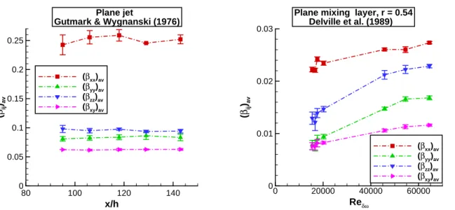
Figures 2, 3 and 4 show the profiles of the coefficientsβij obtained from an analysis of the experiments

of Gutmark and Wygnanski11 _{for the plane jet, of Hussein et al.}14 _{for the axisymmetric jet and of Delville} et al.17 _{for a plane mixing layer at velocity ratio}_r_{= 0}_._{54. Indeed, in all cases there exists a region, where} the coefficientsβij might be considered approximately constant. Nevertheless its extent and pronounciation

depends on the respective flow and the Reynolds-stress component and might be influenced by the experi-mental set-up (Fig. 3) or measurement position, i. e. local Reynolds number (Fig. 4). In agreement with the theoretical considerations, in the jet flows the indicated region occurs at some distance from the cen-terline and extends approximately from the region around the theoretical position of the maximum specific Reynolds-shear stress to the half-width or slightly beyond. In the plane mixing layer it is located around the dividing streamline, covering at least 20−40% of the vorticity thicknessδωin both directions.

Thus, the experimental data confirm the theoretically deduced layer of constant Reynolds-stress anisotrop-ies in turbulent jets and the turbulent plane mixing layer.

IV. Turbulence Structure

IV.A. Reynolds-Stress Anisotropy

As pointed out by Pope,23 _{only the anisotropic part of the specific Reynolds-stress components is effective} in transporting momentum. Hence the accuracy of turbulence models depends on their ability to predict the Reynolds-stress anisotropiesbij correctly, in particular that of the Reynolds-shear stress,bxyorbrz. For

this reason, the Reynolds-stress anisotropies of the investigated flows are deduced from the results for the coefficientsβij in the constant region.

According to Eq. (34), in this region the specific Reynolds stresses all follow the same profile function Gxy(η), differing only in the value of the respective coefficientβij. Hence the definition of the Reynolds-stress

anisotropies (5) yields bij= βij βkk − 1 3δij, (36)

allowing to compute the Reynolds-stress anisotropies directly from the values of the coefficientsβij in the

constant region obtained from the experimental data.

(7)

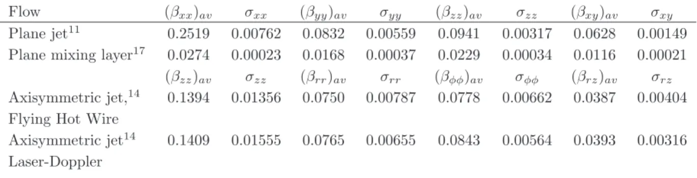
Table 1: Averaged Reynolds-stress coefficients in the constant region.

Flow (βxx)av σxx (βyy)av σyy (βzz)av σzz (βxy)av σxy

Plane jet11 _0.2519 _0.00762 _0.0832 _0.00559 _0.0941 _0.00317 _0.0628 _0.00149 Plane mixing layer17 _0.0274 _0.00023 _0.0168 _0.00037 _0.0229 _0.00034 _0.0116 _0.00021

(βzz)av σzz (βrr)av σrr (βφφ)av σφφ (βrz)av σrz

Axisymmetric jet,14 _0.1394 _0.01356 _0.0750 _0.00787 _0.0778 _0.00662 _0.0387 _0.00404 Flying Hot Wire

Axisymmetric jet14 _0.1409 _0.01555 _0.0765 _0.00655 _0.0843 _0.00564 _0.0393 _0.00316 Laser-Doppler

In order to reduce the uncertainty in the data, the coefficients βij are averaged over the respective

constant region. Since Gutmark and Wygnanski11 _{and Delville et al.}17 _{provide their data at different} downstream positions, the averaging has been carried out for each data set individually. In contrast, Hussein et al.14 _{provide data only at one position, for which they nevertheless checked that self-preservation has} been achieved.

Figure 5 shows the streamwise development of the averaged coefficients (βij)av for the plane-jet data

of Gutmark and Wygnanski11 _{and for the plane mixing-layer data of Delville et al.,}17 _{in which also data} from further upstream positions have been included. As one can see, the plane-jet results seem to be fairly independent of the downstream position, confirming that self-preservation has been achieved, whereas the mixing-layer results still exhibit some variation. In contrast, the standard deviation of the plane-jet data indicated by the error bars is generally larger than that of the plane mixing-layer data.

The largest relative uncertainties are observed for the Reynolds-normal stress in the direction of the predominant mean-velocity gradient, where for the plane-jet data at the most downstream position the standard deviationσyyis approximately 7% of the mean value (βyy)av. For all other components the standard

deviation is of the order of 2% to 3.5% of the corresponding mean value. For the plane mixing-layer data it is of the order of 1% to 2% for all components.

Table 1 contains the averaged Reynolds-stress coefficients (βij)av together with the associated standard

deviationsσij for the different flows. The values for the plane-jet experiment of Gutmark and Wygnanski11

and the plane mixing-layer experiment of Delville et al.17 _{refer to the respective most downstream position} associated with the highest local Reynolds number. For the axisymmetric-jet experiment of Hussein et al.,14the averages of the data obtained by a flying hot-wire and by Laser-Doppler anemometry are provided separately. Note the difference between the coefficients βrr and βφφ, indicating some deviation from the

axisymmetry of the jet.

Table 2 contains the Reynolds-stress anisotropies bij for the different flows inferred from the averaged

coefficients (βij)av in Table 1 according to Eq. (36). For comparison, the boundary-layer values according

to the classical log-law assumption,2 _R

xx : Ryy : Rzz = 4 : 2 : 3, and the Bradshaw hypothesis34 for the

Reynolds-shear stress have been included.

For the axisymmetric jet, the values refer to the average results obtained from the flying hot-wire data and the Laser-Doppler anemometry data of Hussein et al.,14 _{where the values of} _b

rr and bφφ have been

additionally averaged, in order to compensate for the observed deviation from axisymmetry. The ∆bij in

Table 2 refer to an estimate of the uncertainty associated with the averaging of the coefficients βij. They

have been obtained from ∆bij= sµ ∂bij ∂βxx ¯ ¯ ¯ ¯ av σxx ¶2 + µ ∂bij ∂βyy ¯ ¯ ¯ ¯ av σyy ¶2 + µ ∂bij ∂βzz ¯ ¯ ¯ ¯ av σzz ¶2 + µ ∂bij ∂βxy ¯ ¯ ¯ ¯ av σxy ¶2 , (37)

where there is no summation oni andj. The derivatives follow from Eq. (36), relating the Reynolds-stress anisotropies bij to the coefficients βij. Note that Eq. (37) does not allow for a compensation of errors and

thus yields a rather conservative estimate.

An additional cross-comparison of various mixing-layer data has revealed that the experimental results by Delville et al.17 _{deviate from those obtained by Bell and Mehta,}18_Mehta19_{and Tavoularis and Corrsin.}16 _For

(8)

Table 2: Reynolds-stress anisotropies in the constant region.

Flow bxx ∆bxx byy ∆byy bzz ∆bzz bxy ∆bxy

Boundary layer2, 34 _0.111 _– _-0.111 _– ₀ _– _-0.150 _–

Plane jet11 _0.254 _0.011 _-0.139 _0.011 _-0.114 _0.008 _0.146 _0.005

Plane mixing layer17 _0.075 _0.004 _-0.083 _0.004 _0.008 _0.004 _0.173 _0.003 Plane mixing layer16, 18, 19 _0.114 _±₀_.₀₀₅ _-0.085 _±₀_.₀₀₂ _-0.029 _±₀_.₀₀₃ _0.164 _±₀_.₀₁₂

bzz ∆bzz brr ∆brr bφφ ∆bφφ brz ∆brz

Axisymmetric jet14 _0.139 _0.030 _-0.069 _0.022 _-0.069 _0.022 _0.131 _0.014

Table 3: Characteristics of the anisotropy tensor in the constant region.

Flow IIb IIIb λ(1b) λ (b) 2 λ (b) 3 θ Boundary layer2, 34 ₋₀_.₀₃₄₈ ₀ ₀_.₁₈₇ ₋₀_.₁₈₇ ₀ ₋₂₆_.₇o Plane jet11 ₋₀_.₀₆₉₈ ₀_.₀₀₆₅₁ ₀_.₃₀₂ ₋₀_.₁₈₇ ₋₀_.₁₁₅ ₁₈_.₃o Axisymmetric jet14 ₋₀_.₀₃₁₇ ₀_.₀₀₁₈₇ ₀_.₂₀₂ ₋₀_.₁₃₂ ₋₀_.₀₇₀ ₂₅_.₈o

Plane mixing layer17 ₋₀_.₀₃₆₂ ₋₀_.₀₀₀₂₉ ₀_.₁₈₆ ₋₀_.₁₉₄ ₀_.₀₀₈ ₃₂_.₈o

Plane mixing layer16, 18, 19 −0.0374 0.00106 0.206 −0.177 −0.029 29.4o

this reason, an estimate of the anisotropies based on these data together with an estimate of the corresponding uncertainties has been added to Tab. 2. Details are given in.36

Despite the estimated uncertainties in the data, the values in Tab. 2 are supposed to be reliable enough to indicate differences between the turbulence structures of the respective flows.

IV.B. Invariants, Eigenvalues and Principle Axes

For characterising the turbulence structure of the respective flows, the invariants of the anisotropy tensor have been computed according to Eqs. (8) and (9) together with the corresponding eigenvalues. The results are summarised in Tab. 3, where the third eigenvalueλ(3b)follows from the condition of tracelessness. Note that the invariants and eigenvalues for the plane mixing layer, particularly when referring to the data by Delville et al.,17_{are rather close to those for the classical boundary layer assumptions,}2, 34_{implying a similar} turbulence structure in those flows.

This is confirmed by plotting the invariants of the respective flows into the so-called invariant map shown in Fig. 6 (left). Originally derived by Lumley,24 _{this graph represents the domain of physically possible} turbulence states in terms of the invariants of the Reynolds-stress anisotropy tensor. As supposed by the data in Tab. 3, the turbulence states of the boundary layer and the plane mixing layer, particularly when referring to the data of Delville et al.,17 _{are very close to one another, whereas the jet flows are somewhat} different.

The eigenvalues, closely related to the invariants of the Reynolds-stress anisotropy tensor, allow for a geometrical interpretation of the associated Reynolds-stress tensor itself. Since the latter is positive semi-definite, it is associated with a tensor surface representing an ellipsoid. The lengths of its semi-axes are given by the square-root of the respective eigenvalues of the Reynolds-stress tensor that are obtained from the eigenvalues of the corresponding anisotropy tensor according to

λ(iR)= 2k µ λ(ib)+ 1 3 ¶ . (38)

Since eigenvalues and invariants are interrelated, each location in the invariant map, Fig. 6, is thus associated with a particular aspect ratio, i. e. shape, of the corresponding ellipsoid.

However, in order to describe the anisotropy tensor completely, its principal axes are required defined by the respective eigenvectors~x(k)_{. They follow from the anisotropy components in Tab. 2 and the}

(9)

ing eigenvalues in Tab. 3 for the constant region according to bijx(jk)=λ (b) k x (k) i , k= 1,2,3. (39)

Since the flows under investigation are two-dimensional, it suffices to consider the respective eigensystem in the flow plane; the eigenvector~x(3) _{associated with the third eigenvalue}_λ(b)

3 is oriented into the spanwise or circumferential direction, respectively.

Figure 6 (right) shows the principal axes of the anisotropy tensor and, hence, the Reynolds-stress tensor together with the associated ellipses for the different flows with respect to the flow-aligned coordinate system. The semi-axes of the ellipses have been scaled by the specific kinetic turbulence energyk, yielding

x = s λ(1R) k cosφ= s 2 µ λ(1b)+ 1 3 ¶ cosφ, (40) y = s λ(₂R) k sinφ,= s 2 µ λ(₂b)+1 3 ¶ sinφ, 0≤φ≤2π. (41)

As one may already conclude from the eigenvalues of the anisotropy tensor in Tab. 3, the shape of the ellipses is rather similar between the different flows, where the plane jet shows the largest aspect ratio. In contrast, the principal axes of the Reynolds-stress (ansiotropy) tensor obviously have a different inclination against the flow-aligned coordinate system, as indicated in the last column of Tab. 3.

The inclination angle has a major influence on the transport of mean momentum normal to the principal mean-flow direction, which can be seen from the anisotropy component associated with the Reynolds-shear stress. According to the rules of coordinate transformation its value follows from the eigenvalues associated with the flow plane by

b12= ³

λ₁(b)−λ₂(b)´sinθcosθ, (42)

in whichb12=bxy for plane flow andb12=brz for axisymmetric flow, andθ denotes the rotation angle of

the principal axis system against the flow-aligned coordinate system in the flow plane.

Obviously, for given eigenvalues (or invariants, respectively), the Reynolds-shear-stress anisotropy de-pends on the orientation of the principal axes relative to the flow-aligned coordinate system. By definition, b12 = 0 at θ = nπ₂ with n = 0,±1,±2. . ., i.e. in the principal axis system, and reaches its extremes at

θ=π₄ +nπ₂ with n= 0,±1,±2. . ., i.e. atθ=±45o, associated with values b(12ext)=± 1 2 ³ λ(1b)−λ (b) 2 ´ (43) for the the minimum and maximum Reynolds-shear-stress anisotropy, respectively.

Indeed, of all flows investigated, the plane mixing layer shows an inclination angle of the principal axes of the Reynolds-stress anisotropy tensor in the constant region that is closest to the condition of maximum Reynolds-shear-stress anisotropy, particularly when referring to the data of Delville et al.17 _{This e.g., explains} the difference observed between the absolute values ofbxyin the constant region for the boundary layer and

the plane mixing layer, although the eigenvalues and invariants of the Reynolds-stress anisotropy tensor are very similar for both flows. In contrast, the difference of eigenvalues λ(1b)−λ

(b)

2 in the constant region is larger for the plane jet than for the boundary layer, which is reflected by a larger aspect ratio of the ellipsis associated with the corresponding Reynolds-stress tensor, as shown in Fig. 6 (right). However, due to the lower inclination angle of the principal axes for the plane jet, the absolute values ofbxyfor the plane jet and

the boundary layer are very similar.

V. Turbulence Modeling

The above findings imply that for accurately predicting turbulent free-shear flows, the complete informa-tion on the Reynolds-stress anisotropy tensor, at least in the constant region, is required by the respective turbulence model. The corresponding invariants alone, however, do not account for the orientation of the principal axes of the Reynolds-stress tensor and are, hence, insufficient for a complete description of the turbulence structure. The potential improvement will be demonstrated subsequently.

(10)

V.A. Eddy-Viscosity Models

Commonly, the Reynolds-stress tensor is modeled according to the Boussinesq hypothesis, Rij =−2νtSij+2

3kδij, (44)

assuming the Reynolds stresses being proportional to the strain rates Sij = 1 2 µ ∂Ui ∂xj +∂Uj ∂xi ¶ (45) scaled by an eddy viscosity νt. The second term in Eq. (44) corrects for the proper trace of the

Reynolds-stress tensor and is omitted in models that do not providek.

Under the above boundary-layer assumptions there is one dominating strain-rate component,Sxy=1₂∂U_∂y,

so that the corresponding Reynolds-stress tensor simplifies to

R=    2 3k −νt ∂U ∂y 0 −νt∂U_∂y 2₃k 0 0 0 2 3k   . (46) Its eigenvalues λ(1R,2) = 2 3k± ¯ ¯ ¯ ¯νt∂U ∂y ¯ ¯ ¯ ¯ (47) λ(3R) = 2 3k (48)

are associated with principal axes that are inclined byθ=±45o_{against the main-flow direction, depending}

on the sign of the velocity gradient.

Thus, for any flow governed by the boundary-layer assumptions, eddy-viscosity models will not only predict identical Reynolds-normal stresses, but also an identical orientation of the principal axes of the Reynolds-stress tensor relative to the flow-aligned coordinate system. In contrast, the above analysis of experimental data implies different non-identical Reynolds-normal stresses and different orientations of the principal axes of the Reynolds-stress tensor, depending on the particular type of flow.

Nevertheless, considering the Reynolds-shear stress as the most important component, eddy-viscosity models can be calibrated accordingly. Moreover, the models by Spalart and Allmaras37_{and Menter}38_employ the wall-distance for distinguishing boundary layers from other flows, i.e. general free-shear flows.

V.B. Reynolds-Stress Models

Reynolds-stress models do not rely on the Boussinesq hypothesis (44), but involve the solution of the modeled transport equation of the Reynolds stresses, instead. The focus in Reynolds-stress modeling is on the pressure-strain correlation Πij, which is generally modeled according to the analysis of Rotta28as a traceless

tensor. It therefore does not contribute to the budget of the specific kinetic turbulence energyk, but only redistributes it into the different directions, i.e. it alters the eigenvalues and principal axes of the Reynolds-stress (anisotropy) tensor.

For demonstration, the model of Speziale, Sarkar, and Gatski (SSG)39 _{is considered, reading}

ρΠij = − µ C1ρǫ+1 2C ∗ 1ρPkk ¶ bij+C2ρǫ µ bikbkj−1 3bklbklδij ¶ +³C3−C3∗ p bklbkl ´ ρkSij +C4ρk µ bikSjk+bjkSik− 2 3bklSklδij ¶ +C5ρk(bikWjk+bjkWik), (49)

in whichSij denotes the strain rates according to Eq. (45) and

Wij= 1 2 µ ∂Ui ∂xj − ∂Uj ∂xi ¶ (50)

(11)

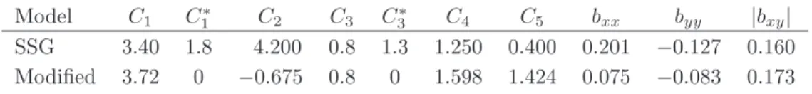
Table 4: Model coefficients and anisotropies

Model C1 C1∗ C2 C3 C3∗ C4 C5 bxx byy |bxy|

SSG 3.40 1.8 4.200 0.8 1.3 1.250 0.400 0.201 −0.127 0.160 Modified 3.72 0 −0.675 0.8 0 1.598 1.424 0.075 −0.083 0.173

are the rotation rates. The model coefficients are given in Tab. 4 together with the associated anisotropies according to the equilibrium condition (12), assuming isotropic dissipation.33 _{Clearly the anisotropies do} not agree with any of the data sets in Tab. 2, except forbxy being close to the plane-mixing layer value in

the fourth row.

In order to demonstrate potential improvement, the model has been recalibrated to the full set of Reynolds-stress anisotropies for the constant region of the plane mixing layer according to the data of Delville et al.17 _{in Tab. 2. The corresponding set of coefficients is termed “Modfied” and is also included} in Tab. 4. This set of coefficients has been implemented into DLR’s flow solver TAU with the SSG-part of the SSG/LRR-ω model,40–42 _{which is active outside boundary layers and, thus, in free shear-layer flows} developing in some distance from solid walls.

Computations have been carried out for the plane mixing layer, specifying inflow conditions according to the experiment by Delville et al.17 as provided on the Turbulence Modeling Resource (TMR) website.43 Profile data have been extracted from the simulations atx= 950mmdownstream of the trailing edge, which is the most downstream position where experimental Reynolds stresses are provided.

Figure 7 shows the comparison of the predicted mean-velocity and Reynolds-stress profiles with the experimental data by Delville et al.17 _{While there is almost no influence of the respective set of coefficients} on the mean-velocity profile, significant differences are observed for the Reynolds-stress profiles. With the SSG-coefficients the peak Reynolds stresses are generally missed, whereas, with the modified coefficients, good agreement with the experimental data is achieved in the center of the mixing layer, except for Rzz

that nevertheless is improved. This confirms that the pressure-strain correlation controls the eigensystem of the Reynolds-stress tensor and underlines the importance of a proper calibration for the Reynolds-stress anisotropies in the constant region.

VI. Conclusions

It has been theoretically shown that, if a flow is governed by the boundary-layer equations and there is an equilibrium between production, dissipation and the pressure-strain correlation, the self-similarity of the mean velocity and the specific Reynolds-shear stress implies the Reynolds-stress anisotropies to be constant. The analysis of experimental data for the plane jet, the axisymmetric jet and the plane mixing layer confirms the existence of such a layer with approximately constant Reynolds-stress anisotropies.

The values of the Reynolds-stress anisotropies obtained in the constant region differ between the flows under investigation. Evaluation of the corresponding invariants, eigenvalues and principal axes shows that, even if the invariants and eigenvalues are similar, the principal axes are inclined differently against the flow-aligned coordinate system, giving rise to different Reynolds-shear stress anisotropy.

Eddy-viscosity models always predict the principal axes of the Reynolds-stress tensor to be inclined by θ =±45o _{against the main-flow direction of a boundary or free-shear layer. In contrast, with}

Reynolds-stress models the predicted Reynolds-Reynolds-stress anisotropy tensor and, hence, its eigensystem are controlled by the pressure-strain correlation. Potential improvement has been demonstrated by recalibrating the SSG-model39 _{according to the Reynolds-stress anisotropies deduced from the experimental data of Delville et} al.17

It is conjectured that observed model failures, like the round-jet/plane-jet anomaly or the under-estimation of Reynolds-shear stress levels in separated shear layers, might be associated with a model calibration that is unsuitable for the respective flow situation. Improvement would therefore require an automatic classification of the respective flow situation and a tailored calibration of the model coefficients for each respective type of flow.

(12)

Acknowledgements

Inspiring discussions with Dr. T. Knopp at DLR G¨ottingen are gratefully acknowledged.

References

1

Bush, B., Chyczewski, T., Duraisamy, K., Eisfeld, B., Rumsey, C., and Smith, B., “Recommendations for Future Efforts in RANS Modeling and Simulation,” Paper submitted to AIAA-SciTech conference 2019.

2

Wilcox, D. C., “Turbulence Modeling for CFD,” DCW Industries, 3rd Edition, 2006. 3

Roshko, A., “Structure of Turbulent Shear Flows: A New Look,”AIAA Journal, Vol. 14, No. 10, 1976, pp. 1349-1357. 4

Görtler, H., “Berechnung von Aufgaben der freien Turbulenz auf Grund eines neuen Näherungsansatzes,”Zeitschrift für Angewandte Mathematik und Mechanik, Vol. 22, 1942, pp. 244-254.

5

Prandtl, L., “Bemerkungen zur Theorie der freien Turbulenz,”Zeitschrift f¨ur Angewandte Mathematik und Mechanik, Vol. 22, 1942, pp. 241-243.

6

F¨orthmann, E., “ ¨Uber turbulente Strahlausbreitung,” Ingenieurarchiv, Vol. 5, 1934, pp. 42-54. 7

Corrsin, S., “Investigation of Flow in an Axially Symmetrical Heated Jet of Air,” NACA Wartime Report W-94, 1943. 8

Liepmann, H. W., Laufer, J., “Investigations of Free Turbulent Mixing,” NACA Technical Note 1257, 1947. 9

Bradbury, L. J. S., “The structure of a self-preserving turbulent plane jet,”Journal of Fluid Mechanics, Vol. 23, 1965, pp. 31-64.

10

Heskestad, G., “Hot-Wire Measurements in a Plane Turbulent Jet,” Journal of Applied Mechanics, Vol. 32, 1965, pp. 721-734.

11

Gutmark, E., Wygnanski, I., “The planar turbulent jet,”Journal of Fluid Mechanics, Vol. 73, 1976, pp. 465-495. 12

Antonia, R. A., Bilger, R. W., “An experimental investigation of an axisymmetric jet in a co-flowing air stream,”Journal of Fluid Mechanics, Vol. 61, 1973, pp. 805-822.

13

Wygnanski, I., Fiedler, H., “Some measurements in the self-preserving jet,”Journal of Fluid Mechanics, Vol. 38, 1969, pp. 577-612.

14

Hussein, H. J., Capp, S. P., George, W. K., “Velocity measurements in a high-Reynolds-number, momentum-conserving, axisymmetric, turbulent jet,”Journal of Fluid Mechanics, Vol. 258, 1994, pp. 31-75.

15

Wygnanski, I., Fiedler, H. E., “The two-dimensional mixing region,”Journal of Fluid Mechanics, Vol. 41, 1970, 327-361. 16

Tavoularis, S., Corrsin, D., “The structure of a turbulent shear layer embedded in turbulence,”Physics of Fluids, Vol. 30, 1987, pp. 3025-3033.

17

Delville, J., Bellin, S., Garm, J. H., Bonnet, J. P., “Analysis of Structures in a Turbulent, Plane Mixing Layer by Use of a Pseudo Flow Visualization Method Based on Hot-Wire Anemometry.” In: Fernholz, H. H., Fiedler, H. E. (Eds.) “Advances in Turbulence 2,” Springer, 1989, pp. 251-256.

18

Bell, J. H., Mehta, R. D., “Development of a Two-Stream Mixing Layer from Tripped and Untripped Boundary Layers,”

AIAA Journal, Vol. 28, 1990, pp. 2034-2042. 19

Mehta, R. D., “Effect of velocity ratio on plane mixing layer development: Influence of the splitter plate wake,” Experi-ments in Fluids, Vol. 10, 1991, pp. 194-204.

20

Benocci, C., Tavoularis, S., Bonnet, J.-P., Leuchter, O., Rodi, W., Onorato, M., van der Vegt, J J. W., Jimenez, J., Smith, P. D., Moser, R, S., Purtell, L. P., “A Selection of Test Cases for the Validation of Large-Eddy Simulations of Turbulent Flow R,” AGARD-Report AGARD-AR-345, 1998.

21

University Madrid, Turbulent Database, AGARD, https://torroja.dmt.upm.es/turbdata/, 2018. 22

Schlichting, H., “Laminare Strahlausbreitung,”, Zeitschrift f¨ur Angewandte Mathematik und Mechanik, Vol. 13, 1933, 260-263.

23

Pope, S. B., “Turbulent Flows,” Cambridge University Press, 2000. 24

Lumley, J. L., “Computational Modeling of Turbulent Flows,”Advances in Applied Mechanics, Vol. 18, 1978, pp. 123-176. 25

Hinze, J. O., “Turbulence,” McGraw-Hill, 2nd Edition, 1975. 26

Rotta, J. C., “Turbulente Str¨omungen,” Teubner, 1972. 27

Launder, B. E., Reece, G. J., and Rodi, W., “Progress in the Development of a Reynolds-Stress Turbulence Closure,”

Journal of Fluid Mechanics, Vol. 68, 1975, pp. 537-566. 28

Rotta, J., “Statistische Theorie nichthomogener Turbulenz,”Zeitschrift f¨ur Physik, Vol. 129, 1951, pp. 547-572. 29

Corrsin, S., “Local isotropy in turbulent shear flow,” NACA Research Memorandum RM 58B11, 1958. 30

Saddoughi, S. G., Veeravalli, S. V., “Local isotropy in turbulent boundary layers at high Reynolds number,”Journal of Fluid Mechanics, Vol. 268, 1994, pp. 333-372.

31

George, W. K., “The Self-Preservation of Turbulent Flows and Its Relation to Initial Conditions and Coherent Structures.” In: George, W. K., Arndt, R., “Advances in Turbulence,”, Springer, 1989, pp. 39-73.

32

Durbin, P. A., Pettersson Reif, B. A., “Statistical Theory and Modeling for Turbulent Flows,” Wiley, Reprint 2003. 33

Abid, R., Speziale, C. G., “Predicting euilibrium states with Reynolds stress closures in channel flow and homogeneous shear flow,”Physics of Fluids A, Vol. 5, 1993, pp. 1776-1782.

34

Bradshaw, P., Ferriss, D. H., Atwell, N. P., “Calculation of boundary-layer development using the turbulent energy equation,”Journal of Fluid Mechanics, Vol. 23, 1967, pp. 593-616.

35

Dairay, T., Obligado, M., Vassilicos, J. J., “Non-equilibrium scaling layws in axisymmetric turbulent wakes,”Journal of Fluid Mechanics, Vol. 781, 2015, pp. 166-195.

36

Eisfeld, B., “Reynolds Stress Anisotropy in Self-Preserving Turbulent Shear Flows,” Internal Report, DLR-IB-AS-BS-2017-106, 2017.

(13)

37

Spalart, P. R. and Allmaras, S. R., “One-Equation Turbulence Model for Aerodynamic Flows,”Recherche A`erospatiale, Vol. 1, 1994, pp. 5-21.

38

Menter, F. R., “Two-Equation Eddy-Viscosity Turbulence Models for Engineering Applications,” AIAA Journal, Vol. 32, No. 8, 1994, pp. 1598-1605

39

Speziale, C. G., Sarkar, S., Gatski, T. B., “Modelling the pressure-strain correlation of turbulence: an invariant dynamical systems approach,”Journal of Fluid MEchanics, Vol. 227, 1991. pp- 245-272.

40

Eisfeld, B., Brodersen, O., “Advances Turbulence Modelling and Stress Analysis for the DLR-F6 Configuration,”AIAA Paper 2005-4727, 2005.

41

C´ecora, R.-D., Radespiel, R., Eisfeld, B., Probst, A., “Differential Reynolds-Stress Modeling for Aeronautics,” AIAA Journal, Vol. 53 No. 3, 2015, pp. 739-755.

42

Eisfeld, B., Rumsey, C., Togiti, V., “Verification and Validation of a Second-Moment Closure Model,”AIAA Journal, Vol. 54 No. 5, 2016, pp. 1524-1541.

43

Rumsey, C. L., “Turbulence Modeling Resource,” https://turbmodels.larc.nasa.gov, cited 15 October 2018.

(14)

y/y_1/2 U /U 0 0 0.5 1 1.5 2 0 0.2 0.4 0.6 0.8 1 x/h = 65 x/h = 76 x/h = 88 x/h = 103 x/h = 118 Theory Plane jet

Gutmark & Wygnanski (1976)

x x x x x x xx x x x x x y/y_1/2 Rx y /U 0 2 0 0.5 1 1.5 0 0.01 0.02 0.03 x/h = 95 x/h = 106 x/h = 118 x/h = 129 x/h = 143 Theory x Plane jet

(a) Plane jet, experiment of Gutmark and Wygnanski.11

r/r_1/2 U /U 0 0 0.5 1 1.5 2 0 0.2 0.4 0.6 0.8 1 Flying hot-wire Laser-Doppler Theory Axisymmetric jet Hussein et al. (1994) r/r_1/2 Rrz /U 0 2 0 0.5 1 1.5 2 0 0.005 0.01 0.015 0.02 0.025 Flying hot-wire Laser-Doppler Theory Axisymmetric jet Hussein et al. (1994)

(b) Axisymmetric jet, experiment of Hussein et al.14

y/δ_ω (U U 0 ) / ∆ Um a x -1 -0.5 0 0.5 1 -0.6 -0.4 -0.2 0 0.2 0.4 0.6 Re_δω = 45743 Re_δω = 54520 Re_δω = 64574 Theory

Plane mixing layer, r = 0.54 Delville et al. (1989) y/δ_ω Rx y /( ∆ Um a x ) 2 -1 0 1 -0.012 -0.01 -0.008 -0.006 -0.004 -0.002 0 Re_δω = 45732 Re_δω = 54520 Re_δω = 64574 Theory

Plane mixing layer, r = 0.54 Delville et al. (1989)

(c) Plane mixing layer, experiment of Delville et al.17

at velocity ratior= 0.54.

Figure 1: Profiles of the non-dimensional mean velocity (left) and Reynolds-shear stress (right). Comparison of experimental data with self-similar solution by G¨ortler.4

(15)

x x x x x x x x x x x _x y/y_1/2 βxy 0 0.5 1 1.5 2 0 0.01 0.02 0.03 0.04 0.05 0.06 0.07 0.08 x/h = 95 x/h = 106 x/h = 118 x/h = 129 x/h = 143 x

(a) Reynolds-shear stress.

x x x x xx x x x x x x x y/y_1/2 βxx 0 0.5 1 1.5 2 0 0.05 0.1 0.15 0.2 0.25 0.3 x/h = 95 x/h = 106 x/h = 118 x/h = 118 x/h = 129 x/h = 143 x

(b) Reynolds-normal stress, streamwise direction.

x x x x x x x _x _x x x x x x y/y_1/2 βyy 0 0.5 1 1.5 2 0 0.05 0.1 0.15 0.2 x/h = 95 x/h = 106 x/h = 118 x/h = 129 x/h = 143 x

(c) Reynolds-normal stress, normal direction.

x x x x xx xx x x x x x y/y_1/2 βzz 0 0.5 1 1.5 2 0 0.05 0.1 0.15 0.2 x/h = 95 x/h = 106 x/h = 118 x/h = 129 x/h = 143 x

(d) Reynolds-normal stress, spanwise direction. Figure 2: Reynolds-stress coefficients βij for the plane jet, experiment of Gutmark and Wygnanski.11 x/h

= distance from virtual origin in terms of orifice width h. Dashed line indicates theoretical position of maximum specific Reynolds-shear stress.

(16)

r/r_1/2 βrz 0 0.5 1 1.5 2 0 0.01 0.02 0.03 0.04 0.05 0.06 Flying hot-wire Laser-Doppler

r/r_1/2 βzz 0 0.5 1 1.5 2 0 0.05 0.1 0.15 0.2 0.25 0.3 Flying hot-wire Laser-Doppler

(b) Reynolds-normal stress, axial direction.

r/r_1/2 βrr 0 0.5 1 1.5 2 0 0.05 0.1 0.15 0.2 Flying hot-wire Laser-Doppler

(c) Reynolds-normal stress, radial direction.

r/r_1/2 βϕϕ 0 0.5 1 1.5 2 0 0.05 0.1 0.15 0.2 Flying hot-wire Laser-Doppler

(d) Reynolds-normal stress, tangential direction. Figure 3: Reynolds-stress coefficients βij for the axisymmetric jet, experiment of Hussein et al.14 Dashed

line indicates theoretical position of maximum specific Reynolds-shear stress.

(17)

y/δ_ω βxy -0.4 -0.2 0 0.2 0.4 0 0.005 0.01 0.015 Re_δω = 45743 Re_δω = 54520 Re_δω = 64574

y/δ_ω βxx -0.4 -0.2 0 0.2 0.4 0 0.01 0.02 0.03 Re_δω = 45743 Re_δω = 54520 Re_δω = 64574

(b) Reynolds-normal stress, streamwise direction.

y/δ_ω βyy -0.4 -0.2 0 0.2 0.4 0 0.005 0.01 0.015 0.02 Re_δω = 45743 Re_δω = 54520 Re_δω = 64574

(c) Reynolds-normal stress, normal direction.

y/δ_ω βzz -0.4 -0.2 0 0.2 0.4 0 0.005 0.01 0.015 0.02 0.025 Re_δω = 45743 Re_δω = 54520 Re_δω = 64574

(d) Reynolds-normal stress, spanwise direction. Figure 4: Reynolds-stress coefficients βij for the plane mixing layer, experiment of Delville et al.17 at

r= 0.54. Reδω = ∆Umaxδω/ν = local Reynolds number.

(18)

x/h ( βij )av 80 100 120 140 0 0.05 0.1 0.15 0.2 0.25 (β_xx)_av (β_yy)_av (β_zz)_av (β_xy)_av Plane jet

(a) Plane jet, experiment of Gutmark and Wygnanski.11

x/h

= distance from virtual origin in terms of nozzle widthh.

Re_δω ( βij )av 0 20000 40000 60000 0 0.01 0.02 0.03 (β_xx)_av (β_yy)_av (β_zz)_av (β_xy)_av

Plane mixing layer, r = 0.54 Delville et al. (1989)

(b) Plane mixing layer, experiment of Delville et al.17 at

r= 0.54. Reδω= ∆Umaxδω/ν= local Reynolds number.

Figure 5: Averaged Reynolds-stress coefficients (βij)av. Error bars indicate standard deviation of averaging.

IIIb IIb

0

Plane jet

(Gutmark & Wygnanski 1976) Axisymmetric jet

(Hussein et al. 1994) Plane mixing layer (Delville et al. 1989) Plane mixing layer (estimate from other data) Boundary layer -1/9 -2/9 -1/3 1/27 2/27 isotropic tw o-com pone nt li mit axis ymm etri c a_x is_y m m . one-component limit

(a) Invariant map.

x y -1 -0.5 0 0.5 1 -1 -0.5 0 0.5 1 Plane jet Axisymmetric jet

Mixing layer (Delville et al.) Mixing layer (other data) Boundary layer

(b) Eigensystems Figure 6: Invariant map and eigensystems of the Reynolds-stress anisotropy tensor.

(19)

η (U - Um ) / ∆ Um a x -1 -0.5 0 0.5 1 -0.5 0 0.5 Experiment SSG Modified

(a) Mean velocity profile. Um=12(Umin+Umax)

η Rx y / [ ∆ Um a x ] 2 -1 -0.5 0 0.5 1 0 0.002 0.004 0.006 0.008 0.01 0.012 Experiment SSG Modified (b)Rxyprofile. η Rx x / [ ∆ Um a x ] 2 -1 -0.5 0 0.5 1 0 0.005 0.01 0.015 0.02 0.025 0.03 0.035 Experiment SSG Modified (c)Rxxprofile. η Ry y / [ ∆ Um a x ] 2 -1 -0.5 0 0.5 1 0 0.005 0.01 0.015 0.02 0.025 0.03 0.035 Experiment SSG Modified (d)Ryyprofile. η Rzz / [ ∆ Um a x ] 2 -1 -0.5 0 0.5 1 0 0.005 0.01 0.015 0.02 0.025 0.03 0.035 Experiment SSG Modified (e)Rzzprofile.

Figure 7: Plane mixing layer, mean-velocity and Reynolds-stress profiles. Comparison of Reynolds-stress model predictions with experimental data by Delville et al.17 at x = 950mm downstream of the splitter plate.

(20)

A. Theoretical Profiles

Based on the assumption of a constant turbulent viscosity, G¨ortler4 _{provides analytical solutions of the} averaged boundary layer equations. These solutions are summarized below for the flows under investigation.

A.A. Plane Jet

• Velocity profile

U

U0(x) = 1−tanh 2

ξ. (51)

• Specific Reynolds-shear stress profile Rxy U2 0(x) = Sb 2ξ1/2 tanhξ ¡1−tanh2ξ¢. (52)

• Velocity scale: Center line velocity

∆Umax(x) =U0(x). (53)

• Non-dimensional normal coordinate

ξ= y y1/2(x) ξ1/2. (54) • Non-dimensional half-width ξ1/2= ln ³_√ 2 + 1´≈0.881. (55) • Spreading rate b S= dy1/2 dx . (56)

A.B. Axisymmetric Jet

• Velocity profile Uz Uz,0(z) = 1 ¡1 4ξ2+ 1 ¢2. (57)