TECHNICAL WORKING PAPER SERIES
ON THE FAILURE OF THE BOOTSTRAP FOR MATCHING ESTIMATORS Alberto Abadie
Guido W. Imbens Technical Working Paper 325 http://www.nber.org/papers/T0325
NATIONAL BUREAU OF ECONOMIC RESEARCH 1050 Massachusetts Avenue
Cambridge, MA 02138 June 2006
We are grateful for comments by Peter Bickel, Stéphane Bonhomme, Whitney Newey, and seminar participants at Princeton, CEMFI, and Harvard/MIT. Financial support for this research was generously provided through NSF grants SES-0350645 (Abadie) and SES-0136789 and SES-0452590 (Imbens). Abadie: John F. Kennedy School of Government, Harvard University, 79 John F. Kennedy Street, Cambridge, MA 02138, and NBER. Electronic c or r e s ponde nc e: [email protected], http://www.ksg.harvard.edu/fs/aabadie/. Imbens: Department of Economics, and Department of Agricultural and Resource Economics, University of California at Berkeley, 330 Giannini Hall, Berkeley, CA 94720-3880, and NBER. Electronic correspondence: [email protected], http://elsa.berkeley.edu/users/imbens/. The views expressed herein are those of the author(s) and do not necessarily reflect the views of the National Bureau of Economic Research.
©2006 by Alberto Abadie and Guido W. Imbens. All rights reserved. Short sections of text, not to exceed two paragraphs, may be quoted without explicit permission provided that full credit, including © notice, is
On the Failure of the Bootstrap for Matching Estimators Alberto Abadie and Guido W. Imbens
NBER Technical Working Paper No. 325 June 2006
JEL No. C14, C21, C52
ABSTRACT
Matching estimators are widely used for the evaluation of programs or treatments. Often researchers use bootstrapping methods for inference. However, no formal justification for the use of the bootstrap has been provided. Here we show that the bootstrap is in general not valid, even in the simple case with a single continuous covariate when the estimator is root-N consistent and asymptotically normally distributed with zero asymptotic bias. Due to the extreme non-smoothness of nearest neighbor matching, the standard conditions for the bootstrap are not satisfied, leading the bootstrap variance to diverge from the actual variance. Simulations confirm the difference between actual and nominal coverage rates for bootstrap confidence intervals predicted by the theoretical calculations. To our knowledge, this is the first example of a root-N consistent and asymptotically normal estimator for which the bootstrap fails to work.
Alberto Abadie
John F. Kennedy School of Government Harvard University
79 John F. Kennedy Street Cambridge, MA 02138 and NBER
[email protected] Guido W. Imbens
Department of Economics
Department of Agricultural and Resource Economics University of California at Berkeley
330 Giannini Hall
Berkeley, CA 94720-3880 and NBER
1
Introduction
Matching methods have become very popular for the estimation of treatment effects.1 Often researchers use bootstrap methods to calculate the standard errors of matching estimators.2 Bootstrap inference for matching estimators has not been formally justified. Because of the non-smooth nature of some matching methods and the lack of evidence that the resulting estimators are asymptotically linear (e.g., nearest neighbor matching with a fixed number of neighbors), there is reason for concern about their validity of the bootstrap in this context.
At the same time, we are not aware of any example where an estimator is root-N
consistent, as well as asymptotically normally distributed with zero asymptotic bias and yet where the standard bootstrap fails to deliver valid confidence intervals.3 This article addresses the question of the validity of the bootstrap for nearest-neighbor matching estimators with a fixed number of neighbors. We show in a simple case with a single continuous covariate that the standard bootstrap does indeed fail to provide asymptoti-cally valid confidence intervals, in spite of the fact that the estimator is root-N consistent and asymptotically normal with no asymptotic bias. We provide some intuition for this failure. We present theoretical calculations for the asymptotic behavior of the difference between the variance of the matching estimator and the average of the bootstrap variance. These theoretical calculations are supported by Monte Carlo evidence. We show that the bootstrap confidence intervals can have over-coverage as well as under-coverage. The
1E.g., Dehejia and Wahba, (1999). See Rosenbaum (2001) and Imbens (2004) for surveys.
2A partial list of recent papers using matching with bootstrapped standard errors includes Agodini and Dynarski (2004), Dehejia and Wahba (1999, 2002), Galasso and Ravaillon (2003), Guarcello, Mealli, and Rosati (2003), Heckman, Ichimura and Todd (1997), Ichino and Becker (2002), Imai (2005), Jalan and Ravallion (1999), Lechner (2002), Myers, Olsen, Seftor, Young, and Tuttle (2002) Pradhan, and Rawlings (2003), Puhani (2002), Sianesi (2004), Smith and Todd (2005), Yamani, Lauer, Starling, Pothier, Tuzcu, Ratliff, Cook, Abdo, McNeil, Crowe, Hobbs, Rincon, Bott-Silverman, McCarthy and Young (2004).
3Familiar examples of failure of the bootstrap for estimators with non-normal limiting distributions arise in the contexts of estimating the maximum of the support of a random variable (Bickel and Freedman, 1981), estimating the average of a variable with infinite variance (Arthreya, 1987), and super-efficient estimation (Beran, 1984). Resampling inference in these contexts can be conducted using alternative methods such as subsampling (Politis and Romano, 1994; Politis, Romano, and Wolf, 1999) and versions of the bootstrap where the size of the bootstrap sample is smaller than the sample size (e.g., Bickel, G¨otze and Van Zwet, 1997). See Hall (1992) and Horowitz (2003) for general discussions.
results do not address whether nearest neighbor estimators with the number of neighbors increasing with the sample size do satisfy asymptotic linearity or whether the bootstrap is valid for such estimators as in practice many researchers have used estimators with very few (e.g., one) nearest neighbor(s).
In Abadie and Imbens (2006) we have proposed analytical estimators of the asymp-totic variance of matching estimators. Because the standard bootstrap is shown to be invalid, together with subsampling (Politis, Romano, and Wolf, 1999) these are now the only available methods of inference that are formally justified.4
The rest of the article is organized as follows. Section 2 reviews the basic notation and setting of matching estimators. Section 3 presents theoretical results on the lack of validity of the bootstrap for matching estimators, along with simulations that confirm the formal results. Section 4 concludes. The appendix contains proofs.
2
Set up
2.1 Basic Model
In this article we adopt the standard model of treatment effects under unconfoundedness (Rubin, 1978; Rosenbaum and Rubin, 1983, Heckman, Ichimura and Todd, 1997, Rosen-baum, 2001, Imbens, 2004). The goal is to evaluate the effect of a treatment on the basis of data on outcomes and covariates for treated and control units. We have a random sam-ple ofN0 units from the control population, and a random sample of N1 units from the treated population, with N =N0+N1. Each unit is characterized by a pair of potential outcomes,Yi(0) andYi(1), denoting the outcomes under the control and active treatment respectively. We observeYi(0) for units in the control sample, andYi(1) for units in the treated sample. For all units we observe a covariate vector,Xi.5 LetWi indicate whether a unit is from the control sample (Wi = 0) or the treatment sample (Wi = 1). For each unit we observe the triple (Xi, Wi, Yi) whereYi =WiYi(1)+(1−Wi)Yi(0) is the observed
4Politis, Romano, and Wolf (1999) show that subsampling produces valid inference for statistics with stable asymptotic distributions.
5To simplify our proof of lack of validity of the bootstrap we will consider in our calculations the case with a scalar covariate. With higher dimensional covariates there is the additional complication of biases that may dominate the asymptotic distribution of matching estimators (Abadie and Imbens, 2006).
outcome. LetX an N-column matrix with column i equal toXi, and similar for Y and
W. Also, let X0 denote the N-column matrix with column i equal to (1−Wi)Xi, and
X1 the N-column matrix with column i equal to WiXi. The following two assumptions are the identification conditions behind matching estimators.
Assumption 2.1: (unconfoundedness) For almost all x, (Yi(1), Yi(0)) is indepen-dent of Wi conditional on Xi =x, or ³ Yi(0), Yi(1) ´ ⊥⊥ Wi ¯ ¯ ¯ Xi =x, (a.s.)
Assumption 2.2: (overlap)For some c >0, and almost all x
c≤Pr(Wi = 1|Xi =x)≤1−c.
In this article we focus on matching estimation of the average treatment effect for the treated:6
τ =E[Yi(1)−Yi(0)|Wi = 1]. (2.1)
A nearest neighbor matching estimator of τ matches each treated unit i to the control unitj with the closest value for the covariate, and then averages the within-pair outcome differences, Yi−Yj, over the N1 matched pairs. Here we focus on the case of matching with replacement, so each control unit can be used as a match for more than one treated units.
Formally, for all treated units i (that is, units with Wi = 1) let Di be the distance between the covariate value for observation i and the covariate value for the closest (control) match:
Di = min
j=1,...,N:Wj=0kXi−Xjk. Then let
J(i) ={j ∈ {1,2, . . . , N}:Wj = 0,kXi−Xjk=Di}
6In many cases, the interest is in the average effect for the entire population. We focus here on the average effect for the treated because it simplifies the calculations below. Since the overall average effect is the weighted sum of the average effect for the treated and the average effect for the controls it suffices to show that the bootstrap is not valid for one of the components.
be the set of closest matches for treated unit i. If unit i is a control unit, then J(i) is defined to be the empty set. When Xi is continuously distributed, the set J(i) will consist of a single index with probability one, but for bootstrap samples there will often be more than one index in this set (because an observation from the original sample may appear multiple times in the bootstrap sample). For each treated unit, i, let
ˆ Yi(0) = 1 #J(i) X j∈J(i) Yj
be the average outcome in the set of the closest matches for observation i, where #J(i) is the number of elements of the set J(i). The matching estimator of τ is then
ˆ τ = 1 N1 X i:Wi=1 ³ Yi−Yˆi(0) ´ . (2.2)
For the subsequent discussion it is useful to write the estimator in a different way. Let
Ki denote the weighted number of times uniti is used as a match (if unit i is a control unit, withKi = 0 if unit i is a treated unit):
Ki = 0 if Wi = 1, X Wj=1 1{i∈ J(j)} 1 #J(j) if Wi = 0. Then we can write
ˆ τ = 1 N1 N X i=1 (Wi−Ki)Yi. (2.3) Let K0 i = 0 if Wi = 1, X Wj=1 1{i∈ J(j)} ³ 1 #J(j) ´2 if Wi = 0.
Abadie and Imbens (2006) prove that under certain conditions (for example, when X is a scalar variable) the nearest-neighbor matching estimator in (2.2) is root-N consistent and asymptotically normal with zero asymptotic bias.7 Abadie and Imbens propose two 7More generally, Abadie and Imbens (2002) propose a bias correction that makes matching estimators root-N consistent and asymptotically normal regardless of the dimension ofX.
variance estimators: b VAI,I = 1 N2 1 N X i=1 ³ Wi−Ki ´2 b σ2(Xi, Wi), and b VAI,II = 1 N2 1 N X i=1 ³ Yi−Yˆi(0)−τˆ ´2 + 1 N2 1 N X i=1 (Ki2−Ki0)bσ2(Xi, Wi), wherebσ2(X
i, Wi) is an estimator of the conditional variance ofYi givenWi and Xi based on matching. Let lj(i) be the j-th closest match to unit i, in terms of the covariates, among the units with the same value for the treatment (that is, units in the treatment groups are matched to units in the treatment group, and units in the control group are matched to units in the control group).8 Define
b σ2(X i, Wi) = J J + 1 Ã Yi− 1 J J X j=1 Ylj(i) !2 . (2.4)
Let V(ˆτ) be the variance of ˆτ, and let V(ˆτ|X,W) the variance of ˆτ conditional on X and W. Abadie and Imbens (2006) show that (under weak regularity conditions) the normalized version of first variance estimator, N1VbAI,I is consistent for the normalized conditional variance,N1V(ˆτ|X,W):
N1(V(ˆτ|X,W)−VbAI,I)−→p 0,
for fixed J as N → ∞. The normalized version of the second variance estimator,
N1VbAI,II, is consistent for the normalized marginal variance, N1V(ˆτ):
N1(V(ˆτ)−VbAI,II) p
−→0,
for fixed J as N → ∞.
8To simplify the notation, here we consider only the case without matching ties. The extension to accommodate ties is immediate (see Abadie, Drukker, Herr, and Imbens, 2004), but it is not required for the purpose of the analysis in this article.
2.2 The Bootstrap
We consider two versions of the bootstrap in this discussion. The first version centers the bootstrap variance at the matching estimate in the original sample. The second version centers the bootstrap variance at the mean of the bootstrap distribution of the matching estimator.
Consider a random sample Z = (X,W,Y) with N0 controls and N1 treated units. The matching estimator, ˆτ, is a functional t(·) of the original sample: ˆτ = t(Z). We construct a bootstrap sample, Zb, with N0 controls and N1 treated by sampling with replacement from the two subsamples. We then calculate the bootstrap estimator, ˆτb, applying the functionalt(·) to the bootstrap sample: ˆτb =t(Zb). The first version of the
bootstrap variance is the second moment of (ˆτb−τˆ) conditional on the sample,Z:
VB,I =vI(Z) =E£(ˆτ b−τˆ)2
¯
¯Z¤. (2.5)
The second version of the bootstrap variance centers the bootstrap variance at the boot-strap mean,E[ˆτb|Z], rather than at the original estimate, ˆτ:
VB,II =vII(Z) = E£(ˆτb−E[ˆτb|Z])2
¯
¯Z¤. (2.6)
Although these bootstrap variances are defined in terms of the original sample Z, in practice an easier way to calculate them is by drawing B bootstrap samples. Given B
bootstrap samples with bootstrap estimates ˆτb, for b= 1, . . . , B, we can obtain unbiased estimators for these two variances as
ˆ VB,I = 1 B B X b=1 (ˆτb−τˆ)2, and ˆ VB,II = 1 B −1 B X b=1 Ã ˆ τb− Ã 1 B B X b=1 ˆ τb !!2 .
We will focus on the first bootstrap variance,VB,I, and its unconditional expectation,
E[VB,I]. We shall show that in general N
1E[VB,I] does not converge toN1V(ˆτ). We will show that in some cases the limit ofN1(E[VB,I]−V(ˆτ)) is positive and that in other cases
this limit is negative. As a result, we will show thatN1VB,I is not a consistent estimator of the limit of N1V(ˆτ). This will indirectly imply that N1VB,II is not consistent either. Because
E£(ˆτb−τˆ)2
¯
¯Z¤≥E£(ˆτb−E[ˆτb|Z])2¯¯Z¤,
it follows thatE[VB,I]≥E[VB,II]. Thus in the cases where the limit ofN
1(E[VB,I]−V(ˆτ)) is smaller than zero, it follows that the limit ofN1(E[VB,II]−V(ˆτ)) is also smaller than zero.
In most standard settings, both centering the bootstrap variance at the estimate in the original sample or at the average of the bootstrap distribution of the estimator lead to valid confidence intervals. In fact, in many settings the average of the bootstrap distribution of an estimator is identical to the estimate in the original sample. For example, if we are interested in constructing a confidence interval for the population meanµ=E[X] given a random sampleX1, . . . , XN, the expected value of the bootstrap statistic, E[ˆµb|X1, . . . , XN], is equal to the sample average for the original sample, ˆµ =
P
iXi/N. For matching estimators, however, it is easy to construct examples where the average of the bootstrap distribution of the estimator differs from the estimate in the original sample. As a result, the two bootstrap variance estimators will lead to different confidence intervals with potentially different coverage rates.
3
An Example where the Bootstrap Fails
In this section we discuss in detail a specific example where we can calculate the limits of N1V(ˆτ) and N1E[VB,I] and show that they differ.
3.1 Data Generating Process
We consider the following data generating process:
Assumption 3.1: The marginal distribution of the covariate X is uniform on the in-terval [0,1]
Assumption 3.3: The propensity score e(x) = Pr(Wi = 1|Xi = x) is constant as a function of x.
Assumption 3.4: The distribution of Yi(1) is degenerate with Pr(Yi(1) = τ) = 1, and the conditional distribution ofYi(0) given Xi =x is normal with mean zero and variance one.
The implication of Assumptions 3.2 and 3.3 is that the propensity score ise(x) = α/(1 +
α).
3.2 Exact Variance and Large Sample Distribution
The data generating process implies that conditional on X = x the treatment effect is equal to E[Y(1) −Y(0)|X = x] = τ for all x. Therefore, the average treatment effect for the treated is equal to τ. Under this data generating process PiWiYi/N1 =
P
iWiYi(1)/N1 =τ, which along with equation (2.3) implies: ˆ τ −τ =− 1 N1 N X i=1 KiYi.
Conditional on X and W the only stochastic component of ˆτ is Y. By Assumption 3.4 the Yi-s are mean zero, unit variance, and independent of X. Thus E[ˆτ −τ|X,W] = 0. Because (i) E[YiYj|Wi = 0,X,W] = 0 for i =6 j, (ii) E[Yi2|Wi = 0,X,W] = 1 and (iii)
Ki is a deterministic function of X and W, it also follows that the conditional variance of ˆτ given X and W is V(ˆτ|X,W) = 1 N2 1 N X i=1 K2 i.
Because V(E[ˆτ|X,W]) = V(τ) = 0, the (exact) unconditional variance of the matching estimator is therefore equal to the expected value of the conditional variance:
V(ˆτ) = N0 N2 1 E£K2 i|Wi = 0 ¤ . (3.7)
Lemma 3.1: (Exact Variance of Matching Estimator) Suppose that Assumptions 2.1, 2.2, and 3.1-3.4 hold. Then
(i) the exact variance of the matching estimator is V(ˆτ) = 1 N1 +3 2 (N1−1)(N0+ 8/3) N1(N0+ 1)(N0+ 2) , (3.8) (ii) as N → ∞, N1V(ˆτ)→1 + 3 2α, (3.9) and (iii), √ N1(ˆτ −τ)−→ Nd µ 0,1 + 3 2α ¶ .
All proofs are given in the Appendix. 3.3 The Bootstrap Variance
Now we analyze the properties of the bootstrap variance, VB,I in (2.5). As before, let
Z= (X,W,Y) denote the original sample. We will look at the distribution of statistics both conditional on the original sample, as well as over replications of the original sample drawn from the same distribution. Notice that
E£VB,I¤=E£E£(ˆτ b−τˆ)2
¯
¯Z¤¤=E£(ˆτb −τˆ)2¤ (3.10) is the expected bootstrap variance. The following lemma establishes the limit ofN1E[VB,I] under our data generating process.
Lemma 3.2: (Bootstrap Variance I)Suppose that Assumptions 3.1-3.4 hold. Then, as N → ∞: N1E[VB,I]→1 + 3 2α 5 exp(−1)−2 exp(−2) 3 (1−exp(−1)) + 2 exp(−1). (3.11) Recall that the limit of the normalized variance of ˆτ is 1 + (3/2)α. For small values of
α the limit of the expected bootstrap variance exceeds the limit variance by the third term in (3.11), 2 exp(−1) ' 0.74, or 74%. For large values of α the second term in (3.11) dominates and the ratio of the limit expected bootstrap and limit variance is equal to the factor in the second term of (3.11) multiplying (3/2)α. Since (5 exp(−1)−
2 exp(−2))/(3 (1−exp(−1)))'0.83, it follows that asα increases, the ratio of the limit expected bootstrap variance to the limit variance asymptotes to 0.83, suggesting that in large samples the bootstrap variance can under as well as over estimate the true variance. So far, we have established the relation between the limiting variance of the estimator and the limit of the average bootstrap variance. We end this section with a discussion of the implications of the previous two lemmas for the validity of the bootstrap. The first version of the bootstrap provides a valid estimator of the asymptotic variance of the simple matching estimator if:
N1 ³ E£(τbb−bτ)2 ¯ ¯Z¤−V(bτ)´ p −→0.
Lemma 3.1 shows that:
N1V(τb)−→1 + 3 2α. Lemma 3.2 shows that
N1E £ (bτb −bτ)2 ¤ −→1 + 3 2α 5 exp(−1)−2 exp(−2) 3(1−exp(−1)) + 2 exp(−1).
Assume that the first version of the bootstrap provides a valid estimator of the asymptotic variance of the simple matching estimator. Then,
N1E £ (bτb−τb)2 ¯ ¯Z¤ p −→1 + 3 2α.
Because N1E[(τbb−bτ)2|Z] ≥ 0, it follows by Portmanteau Lemma (see, e.g., van der Vaart, 1998, page 6) that, asN → ∞,
1 + 3 2α≤limE h N1E £ (τbb−bτ)2 ¯ ¯Z¤ i= limN1E£(τbb−bτ)2¤ = 1 + 3 2α 5 exp(−1)−2 exp(−2) 3(1−exp(−1)) + 2 exp(−1). However, the algebraic inequality
1 + 3 2α≤1 + 3 2α 5 exp(−1)−2 exp(−2) 3(1−exp(−1)) + 2 exp(−1),
does not hold for large enoughα. As a result, the first version of the bootstrap does not provide a valid estimator of the asymptotic variance of the simple matching estimator.
The second version of the bootstrap provides a valid estimator of the asymptotic variance of the simple matching estimator if:
N1 ³ E£(τbb−E[bτb|Z])2 ¯ ¯Z¤−V(τb)´ p −→0.
Assume that the second version of the bootstrap provides a valid estimator of the asymp-totic variance of the simple matching estimator. Then,
N1E £ (bτb−E[bτb|Z])2 ¯ ¯Z¤ p −→1 + 3 2α.
Notice thatE[(bτb−E[bτb|Z])2|Z]≤E[(bτb−τb)2|Z]. By Portmanteau Lemma, asN → ∞ 1 + 3 2α≤lim infE h N1E £ (bτb−E[bτb|Z])2 ¯ ¯Z¤ i≤limEhN1E£(τbb−bτ)2¯¯Z¤ i = limN1E £ (bτb−bτ)2 ¤ = 1 + 3 2α 5 exp(−1)−2 exp(−2) 3(1−exp(−1)) + 2 exp(−1). Again, this inequality does not hold for large enough α. As a result, the second version of the bootstrap does not provide a valid estimator of the asymptotic variance of the simple matching estimator.
3.4 Simulations
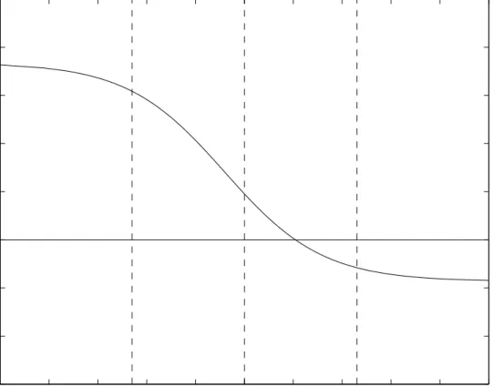
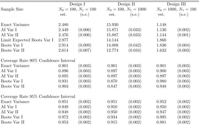
We consider three designs: N0 =N1 = 100 (Design I), N0 = 100,N1 = 1000 (Design II), and N0 = 1000, N1 = 100 (Design III), We use 10,000 replications, and 100 bootstrap samples in each replication. These designs are partially motivated by Figure 1, which gives the ratio of the limit of the expectation of the bootstrap variance (given in equation (3.11)) to limit of the actual variance (given in equation (3.9)), for different values ofα. On the horizontal axis is the log ofα. As αconverges to zero the variance ratio converges to 1.74; at α = 1 the variance ratio is 1.19; and as α goes to infinity the variance ratio converges to 0.83. The vertical dashed lines indicate the three designs that we adopt in our simulations: α= 0.1, α= 1, and α= 10.
The simulation results are reported in Table 1. The first row of the table gives normalized exact variances, N1V(ˆτ), calculated from equation (3.8). The second and third rows present averages (over the 10,000 simulation replications) of the normalized
variance estimators from Abadie and Imbens (2006). The second row reports averages of
N1VbAI,I and the third row reports averages of N1VbAI,II. In large samples, N1VbAI,I and
N1VbAI,II are consistent forN1V(ˆτ|X,W) andN1V(ˆτ), respectively. Because, for our data generating process, the conditional average treatment effect is zero for all values of the covariates, N1VbAI,I and N1VbAI,II converge to the same parameter. Standard errors (for the averages over 10,000 replications) are reported in parentheses. The first three rows of Table 1 allow us to assess the difference between the averages of the Abadie-Imbens (AI) variance estimators and the theoretical variances. For example, for Design I, the normalized AI Var I estimator (N1VbAI,I) is on average 2.449, with a standard error of 0.006. The theoretical variance is 2.480, so the difference between the theoretical and AI variance I is approximately 1%, although it is statistically significant at about 5 standard errors. Given the theoretical justification of the variance estimator, this difference is a finite sample phenomenon.
The fourth row reports the limit of normalized expected bootstrap variance,N1E[VB,I], calculated as in (3.11). The fifth and sixth rows give normalized averages of the estimated bootstrap variances,N1VbB,I and N1VbB,II, over the 10,000 replications. These variances are estimated for each replication using 100 bootstrap samples, and then averaged over all replications. Again it is interesting to compare the average of the estimated bootstrap variance in the fifth row to the limit of the expected bootstrap variance in the fourth row. The differences between the fourth and fifth rows are small (although significantly different from zero as a result of the small sample size). The limited number of bootstrap replications makes these averages noisier than they would otherwise be, but it does not affect the average difference. The results in the fifth row illustrate our theoretical calcula-tions in Lemma 3.2: the average bootstrap variance can over-estimate or under-estimate the variance of the matching estimator.
The next two panels of the table report coverage rates, first for nominal 90% confi-dence intervals and then for nominal 95% conficonfi-dence intervals. The standard errors for the coverage rates reflect the uncertainty coming from the finite number of replications (10,000). They are equal to pp(1−p)/R where for the second panel p = 0.9 and for
the third panelp= 0.95, andR= 10,000 is the number of replications.
The first rows of the last two panels of Table 1 report coverage rates of 90% and 95% confidence intervals constructed in each replication as the point estimate, ˆτ, plus/minus 1.645 and 1.96 times the square root of the variance in (3.8). The results show coverage rates which are statistically indistinguishable from the nominal levels, for all three designs and both levels (90% and 95%). The second row of the second and third panels of Table 1 report coverage rates for confidence intervals calculated as in the preceding row but using the estimator VbAI,I in (2.5). The third row report coverage rates for confidence intervals constructed with the estimatorVbAI,II in (2.6). Both VbAI,I and VbAI,II produce confidence intervals with coverage rates that are statistically indistinguishable from the nominal levels.
The last two rows of the second panel of Table 1 report coverage rates for bootstrap confidence intervals obtained by adding and subtracting 1.645 times the square root of the estimated bootstrap variance in each replication, again over the 10,000 replications. The third panel gives the corresponding numbers for 95% confidence intervals.
Our simulations reflect the lack of validity of the bootstrap found in the theoreti-cal theoreti-calculations. Coverage rates of confidence intervals constructed with the bootstrap estimators of the variance are different from nominal levels in substantially important and statistically highly significant magnitudes. In Designs I and III the bootstrap has coverage larger the nominal coverage. In Design II the bootstrap has coverage smaller than nominal. In neither case the difference is huge, but it is important to stress that this difference will not disappear with a larger sample size, and that it may be more substantial for different data generating processes.
The bootstrap calculations in this table are based on 100 bootstrap replications. In-creasing the number of bootstrap replications significantly for all designs was infeasible as matching is already computationally expensive.9 We therefore investigated the im-plications of this choice for Design I, which is the fastest to run. For the same 10,000
9Each calculation of the matching estimator requires N
1 searches for the minimum of an array of lengthN0, so that withB bootstrap replications andR simulations one quickly requires large amounts of computer time.
replications we calculated both the coverage rates for the 90% and 95% confidence in-tervals based on 100 bootstrap replications and based on 1,000 bootstrap replications. For the confidence intervals based on VbB,I the coverage rate for a 90% nominal level was 0.002 (s.e. 0.001) higher with 1,000 bootstrap replications than with 100 bootstrap replications. The coverage rate for the 95% confidence interval was 0.003 (s.e., 0.001) higher with 1,000 bootstrap replications than with 100 bootstrap replications. Because the difference between the bootstrap coverage rates and the nominal coverage rates for this design are 0.031 and 0.022 for the 90% and 95% confidence intervals respectively, the number of bootstrap replications can only explain approximately 6-15% of the difference between the bootstrap and nominal coverage rates. We therefore conclude that using more bootstrap replications would not substantially change the results in Table 1.
4
Conclusion
In this article we prove that the bootstrap is not valid for the standard nearest-neighbor matching estimator with replacement. This is a somewhat surprising discovery, because in the case with a scalar covariate the matching estimator is root-N consistent and asymptotically normally distributed with zero asymptotic bias. However, the extreme non-smooth nature of matching estimators and the lack of evidence that the estimator is asymptotically linear explain the lack of validity of the bootstrap. We investigate a special case where it is possible to work out the exact variance of the estimator as well as the limit of the average bootstrap variance. We show that in this case the limit of the average bootstrap variance can be greater or smaller than the limit variance of the matching estimator. This implies that the standard bootstrap fails to provide valid inference for the matching estimator studied in this article. A small Monte Carlo study supports the theoretical calculations. The implication for empirical practice of these results is that for nearest-neighbor matching estimators with replacement one should use the variance estimators developed by Abadie and Imbens (2006) or the subsampling bootstrap (Politis, Romano and Wolf, 1999). It may well be that if the number of neighbors increases with the sample size the matching estimator does become asymptotically linear and sufficiently
regular for the bootstrap to be valid. However, the increased risk of a substantial bias has led many researchers to focus on estimators where the number of matches is very small, often just one, and the asymptotics based on an increasing number of matches may not provide a good approximation in such cases.
Finally, our results cast doubts on the validity of the standard bootstrap for other estimators that are asymptotically normal but not asymptotically linear (see, e.g., Newey and Windmeijer, 2005).
Appendix
Before proving Lemma 3.1 we introduce some notation and preliminary results. LetX1, . . . , XN be a
random sample from a continuous distribution. Let Mj be the index of the closest match for unit j.
That is, if Wj = 1, then Mj is the unique index (ties happen with probability zero), with WMj = 0, such thatkXj−XMjk ≤ kXj−Xik, for allisuch thatWi= 0. IfWj= 0, then Mj = 0. LetKi be the number of times uniti is the closest match for a treated observation:
Ki= (1−Wi) N
X
j=1
Wj1{Mj=i}.
Following this definitionKi is zero for treated units. Using this notation, we can write the estimator for
the average treatment effect on the treated as: ˆ τ = 1 N1 N X i=1 (Wi−Ki)Yi. (A.1)
Also, letPi be the probability that the closest match for a randomly chosen treated unit j is unit i,
conditional on both the vector of treatment indicators W and on vector of covariates for the control unitsX0:
Pi= Pr(Mj =i|Wj= 1,W,X0). For treated units we definePi= 0.
The following lemma provides some properties of the order statistics of a sample from the standard uniform distribution.
Lemma A.1: Let X(1)≤X(2)≤ · · · ≤X(N) be the order statistics of a random sample of sizeN from
a standard uniform distribution,U(0,1). Then, for1≤i≤j ≤N,
E[X(ri)(1−X(j))s] =
i[r](N−j+ 1)[s] (N+ 1)[r+s] ,
where for a positive integer,a, and a non-negative integer,b: a[b]= (a+b−1)!/(a−1)!. Moreover, for 1≤i≤N,X(i)has a Beta distribution with parameters(i, N−i+ 1); for 1≤i≤j ≤N,(X(j)−X(i))
has a Beta distribution with parameters(j−i, N−(j−i) + 1).
Proof: All the results of this lemma, with the exception of the distribution of differences of order statistics, appear in Johnson, Kotz, and Balakrishnan (1994). The distribution of differences of order statistics can be easily derived from the joint distribution of order statistics provided in Johnson, Kotz,
and Balakrishnan (1994). ¤
Notice that the lemma implies the following results: E[X(i)] = i N+ 1 for 1≤i≤N, E[X2 (i)] = i(i+ 1) (N+ 1)(N+ 2) for 1≤i≤N, E[X(i)X(j)] = i(j+ 1) (N+ 1)(N+ 2) for 1≤i≤j≤N.
First we investigate the first two moments ofKi, starting by studying the conditional distribution ofKi
Lemma A.2: (Conditional Distribution and Moments of Ki)
Suppose that assumptions 3.1-3.3 hold. Then, the distribution ofKi conditional on Wi= 0,W, andX0
is binomial with parameters(N1, Pi):
Ki|Wi= 0,W,X0∼ B(N1, Pi).
Proof: By definition Ki = (1−Wi)
PN
j=1Wj1{Mj =i}. The indicator 1{Mj =i} is equal to one if the closest control unit forXj isi. This event has probability Pi. In addition, the events 1{Mj1 =i}
and 1{Mj2 =i}, for Wj1 =Wj2 = 1 andj16=j2, are independent conditional on Wand X0. Because
there areN1 treated units the sum of these indicators follows a binomial distribution with parameters
N1andPi. ¤
This implies the following conditional moments forKi: E[Ki|W,X0] = (1−Wi)N1Pi, E[Ki2|W,X0] = (1−Wi) ¡ N1Pi+N1(N1−1)Pi2 ¢ .
To derive the marginal moments ofKi we need first to analyze the properties of the random variable
Pi. Exchangeability of the units implies that the marginal expectation ofPi given N0, N1 andWi = 0
is equal to 1/N0. To derive the second moment of Pi it is helpful to express Pi in terms of the order
statistics of the covariates for the control group. For control unitiletι(i) be the order of the covariate for theith unit among control units:
ι(i) =
N
X
j=1
(1−Wj) 1{Xj≤Xi}.
Furthermore, let X0(k) be the kth order statistic of the covariates among the control units, so that
X0(1) ≤ X0(2) ≤ . . . X0(N0), and for control units X0(ι(i)) = Xi. Ignoring ties, a treated unit with
covariate valuexwill be matched to control unitiif X0(ι(i)−1)+X0(ι(i))
2 ≤x≤
X0(ι(i)+1)+X0(ι(i))
2 ,
if 1< ι(i)< N0. Ifι(i) = 1, then xwill be matched to unitiif
x≤ X0(2)+X0(1)
2 ,
and ifι(i) =N0,xwill be matched to unitiif
X0(N0−1)+X0(N0)
2 < x.
To get the value of Pi we need to integrate the density ofX conditional onW = 1,f1(x), over these sets. With a uniform distribution for the covariates in the treatment group (f1(x) = 1, forx∈[0,1]), we get the following representation forPi:
Pi= (X0(2)+X0(1))/2 if ι(i) = 1, ¡ X0(ι(i)+1)−X0(ι(i)−1) ¢ /2 if 1< ι(i)< N0, 1−(X0(N0−1)+X0(N0))/2 if ι(i) =N0. (A.2) Lemma A.3: (Moments of Pi)
Suppose that Assumptions 3.1–3.3 hold. Then
(i), the second moment of Pi conditional onWi= 0 is
E[Pi2|Wi= 0] = 3N0+ 8
and(ii), the Mth moment of Pi is bounded by E[PM i |Wi= 0]≤ µ 1 +M N0+ 1 ¶M .
Proof: First, consider (i). Conditional onWi= 0,Xi has a uniform distribution on the interval [0,1].
Using Lemma A.1 and equation (A.2), for interiori(isuch that 1< ι(i)< N0), we have that E[Pi|1< ι(i)< N0, Wi= 0] = 1 N0+ 1, and E£P2 i|1< ι(i)< N0, Wi = 0 ¤ = 3 2 1 (N0+ 1)(N0+ 2) .
For the smallest and largest observations:
E[Pi|ι(i)∈ {1, N0}, Wi= 0] = 3 2 1 N0+ 1 , and E[Pi2|ι(i)∈ {1, N0}, Wi= 0] = 7 2(N0+ 1)(N0+ 2).
Averaging over all units includes two units at the boundary andN0−2 interior values, we obtain: E[Pi|Wi= 0] = N0−2 N0 1 (N0+ 1) + 2 N0 3 2 1 (N0+ 1) = 1 N0 , and E[P2 i|Wi= 0] = N0−2 N0 3 2 1 (N0+ 1)(N0+ 2)+ 2 N0 7 2 1 (N0+ 1)(N0+ 2) = 3N0+ 8 2N0(N0+ 1)(N0+ 2). For (ii) notice that
Pi= (X0(2)+X0(1))/2≤X0(2) if ι(i) = 1, ¡ X0(ι(i)+1)−X0(ι(i)−1) ¢ /2≤¡X0(ι(i)+1)−X0(ι(i)−1) ¢ if 1< ι(i)< N0, 1−(X0(N0−1)+X0(N0))/2≤1−X0(N0−1) if ι(i) =N0. (A.3) Because the right-hand sides of the inequalities in equation (A.3) all have a Beta distribution with parameters (2, N0−1), the moments ofPi are bounded by those of a Beta distribution with parameters
2 andN0−1. TheMth moment of a Beta distribution with parametersαandβis QM−1
j=0 (α+j)/(α+β+j). This is bounded by (α+M−1)M/(α+β)M, which completes the proof of the second part of the Lemma.
¤
Proof of Lemma 3.1:
First we prove (i). The first step is to calculate E[K2
i|Wi = 0]. Using Lemmas A.2 and A.3, E[Ki2|Wi= 0] =N1E[Pi|Wi= 0] +N1(N1−1)E[Pi2|Wi= 0] =N1 N0 + 3 2 N1(N1−1)(N0+ 8/3) N0(N0+ 1)(N0+ 2) . Substituting this into (3.7) we get:
V(ˆτ) = N0 N2 1 E[Ki2|Wi= 0] = 1 N1 + 3 2 (N1−1)(N0+ 8/3) N1(N0+ 1)(N0+ 2),
proving part (i).
Next, consider part (ii). Multiply the exact variance of ˆτ byN1and substituteN1=α N0 to get
N1V(ˆτ) = 1 + 3 2
(α N0−1)(N0+ 8/3) (N0+ 1)(N0+ 2) . Then take the limit asN0→ ∞to get:
lim
N→∞N1V(ˆτ) = 1 + 3 2α.
Finally, consider part (iii). Let S(r, j) be a Stirling number of the second kind. TheMth moment of Ki givenWandX0 is (Johnson, Kotz, and Kemp, 1993):
E[KM i |X0, Wi= 0] = M X j=0 S(M, j)N0!Pij (N0−j)! .
Therefore, applying Lemma A.3 (ii), we obtain that the moments ofKi are uniformly bounded:
E[KM i |Wi= 0] = M X j=0 S(M, j)N0! (N0−j)! E[P j i|Wi= 0]≤ M X j=0 S(M, j)N0! (N0−j)! µ 1 +M N0+ 1 ¶j ≤ M X j=0 S(M, j)(1 +M)j. Notice that E " 1 N1 N X i=1 K2 i # =N0 N1 E[K2 i|Wi= 0]→1 + 3 2α, V Ã 1 N1 N X i=1 K2 i ! ≤ N0 N2 1 V(K2 i|Wi= 0)→0, because cov(K2
i, Kj2|Wi=Wj= 0, i6=j)≤0 (see Joag-Dev and Proschan, 1983). Therefore:
1 N1 N X i=1 K2 i p →1 +3 2α. (A.4) Finally, we write ˆ τ−τ= 1 N1 N X i=1 ξi,
where ξi = −KiYi. Conditional on X and W the ξi are independent, and the distribution of ξi is
degenerate at zero forWi= 1 and normalN(0, Ki2) forWi= 0. Hence, for anyc∈R:
Pr à ³ 1 N1 N X i=1 Ki2 ´−1/2p N1(ˆτ−τ)≤c ¯ ¯ ¯X,W ! = Φ(c),
where Φ(·) is the cumulative distribution function of a standard normal variable. Integrating over the distribution ofXandWyields:
Pr à ³ 1 N1 N X i=1 Ki2 ´−1/2p N1(ˆτ−τ)≤c ! = Φ(c).
Now, Slustky’s Theorem implies (iii). ¤
Next we introduce some additional notation. LetRb,i be the number of times unitiis in the bootstrap
sample. In addition, letDb,i be an indicator for inclusion of unit i in the bootstrap sample, so that
Db,i = 1{Rb,i > 0}. Let Nb,0 = PN
i=1(1−Wi)Db,i be the number of distinct control units in the bootstrap sample. Finally, define the binary indicatorBi(x), fori= 1. . . , N to be the indicator for the
event that in the bootstrap sample a treated unit with covariate valuexwould be matched to unit i. That is, for this indicator to be equal to one the following three conditions need to be satisfied: (i) unit iis a control unit, (ii) unitiis in the bootstrap sample, and (iii) the distance betweenXi andxis less
than or equal to the distance betweenxand any other control unit in the bootstrap sample. Formally:
Bi(x) =
½
1 if |x−Xi|= mink:Wk=0,Db,k=1|x−Xk|, and Db,i= 1, Wi= 0, 0 otherwise.
For theN units in the original sample, letKb,i be the number of times unitiis used as a match in the
bootstrap sample. Kb,i= N X j=1 WjBi(Xj)Rb,j. (A.5)
We can write the estimated treatment effect in the bootstrap sample as ˆ τb= 1 N1 N X i=1 WiRb,iYi−Kb,iYi.
BecauseYi(1) =τ by Assumption 3.4, and
PN i=1WiRb,i=N1, then ˆ τb−τ =− 1 N1 N X i=1 Kb,iYi.
The difference between the original estimate ˆτ and the bootstrap estimate ˆτb is
ˆ τb−τˆ= 1 N1 N X i=1 (Ki−Kb,i)Yi= 1 α N0 N X i=1 (Ki−Kb,i)Yi.
We will calculate the expectation
N1E[VB,I] =N1·E[(ˆτb−τˆ)2] = N1 α2N2 0 E N X i=1 N X j=1 (Ki−Kb,i)Yi(Kj−Kb,j)Yj .
Using the facts thatE[Y2
i |X,W, Wi = 0] = 1, and E[YiYj|X,W, Wi = Wj = 0] = 0 ifi 6= j, this is equal to N1E[VB,I] = 1 αE £ (Kb,i−Ki)2|Wi= 0 ¤ .
The first step in deriving this expectation is to establish some properties ofDb,i,Rb,i,Nb,0, andBi(x).
Lemma A.4: (Properties of Db,i, Rb,i,Nb,0, andBi(x))
Suppose that Assumptions 3.1-3.3 hold. Then, forw∈ {0,1}, andn∈ {1, . . . , N0} (i)
(ii) Db,i|Wi=w,Z∼ B ¡ 1,1−(1−1/Nw)Nw ¢ , (iii) Pr(Nb,0=n) = µ N0 N0−n ¶ n! NN0 0 S(N0, n), (iv) Pr(Bi(Xj) = 1|Wj= 1, Wi= 0, Db,i= 1, Nb,0) = 1 Nb,0 , (v)forl6=j Pr(Bi(Xl)Bi(Xj) = 1|Wj=Wl= 1, Wi= 0, Db,i= 1, Nb,0) = 3Nb,0+ 8 2Nb,0(Nb,0+ 1)(Nb,0+ 2), (vi) E[Nb,0/N0] = 1−(1−1/N0)N0 →1−exp(−1), (vii) 1 N0 V(Nb,0) = (N0−1) (1−2/N0)N0+ (1−1/N0)N0−N0(1−1/N0)2N0→exp(−1)(1−2 exp(−1)).
Proof: Parts (i), (ii), and (iv) are trivial. Part (iii) follows easily from equation (3.6) in page 110 of Johnson and Kotz (1977). Next, consider part (v). First condition onX0bandWb (the counterparts of
X0 andWin theb-th bootstrap sample), and suppose thatDb,i= 1. The event that a randomly chosen
treated unit will be matched to control uniticonditional on X0b andWb depends on the difference in
order statistics of the control units in the bootstrap sample. The equivalent in the original sample is Pi. The only difference is that the bootstrap control sample is of sizeN0,b. The conditional probability
that two randomly chosen treated units are both matched to control unitiis the square of the difference in order statistics. It marginal expectation is the equivalent in the bootstrap sample ofE[P2
i|Wi = 0],
again with the sample size scaled back toNb,0. Parts (vi) and (vii) can be derived by making use of
equation (3.13) on page 114 in Johnson and Kotz (1977). ¤
Next, we prove a general result for the bootstrap. Consider a sample of sizeN, indexed byi= 1, . . . , N. LetDb,i be an indicator whether observation i is in bootstrap sample b. Let Nb =
PN
i=1Db,i be the number of distinct observations in bootstrap sampleb.
Lemma A.5: (Bootstrap)For all m≥0:
E ·µ N−Nb N ¶m¸ →exp(−m), and E ·µ N Nb ¶m¸ → µ 1 1−exp(−1) ¶m .
Proof: From parts (vi) and (vii) of Lemma A.4 we obtain that (N −Nb)/N p
→ exp(−1). By the Continuous Mapping Theorem,N/Nb→p 1/(1−exp(−1)). To obtain convergence of moments it suffices
that, for anym≥0,E[((N−Nb)/N)m] andE[(N/Nb)m] are uniformly bounded inN (see, e.g., van der
((N−Nb)/N)m≤1. ForE[(N/Nb)m] the proof is a little bit more complicated. As before, it is enough
to show that E[(N/Nb)m] is uniformly bounded for N ≥ 1. Let λ(N) = (1−1/N)N. Notice that
λ(N)<exp(−1) for allN≥1. Let 0< θ <exp(1)−1. Notice that, 1−(1 +θ)λ(N)>0. Therefore:
E ·µ N Nb ¶m¸ =E ·µ N Nb ¶mµ 1 ½ N Nb < 1 1−(1 +θ)λ(N) ¾ + 1 ½ N Nb ≥ 1 1−(1 +θ)λ(N) ¾¶¸ ≤ µ 1 1−(1 +θ) exp(−1) ¶m +E ·µ N Nb ¶m¯ ¯ ¯N Nb ≥ 1 1−(1 +θ)λ(N) ¸ Pr µ N Nb ≥ 1 1−(1 +θ)λ(N) ¶ ≤ µ 1 1−(1 +θ) exp(−1) ¶m +NmPr µ N Nb ≥ 1 1−(1 +θ)λ(N) ¶ .
Therefore, for the expectationE[(N/Nb)m] to be uniformly bounded, it is sufficient that the probability
Pr(N/Nb ≥(1−(1 +θ)λ(N))−1) converges to zero at an exponential rate asN → ∞. Notice that
Pr µ N Nb ≥ 1 1−(1 +θ)λ(N) ¶ = Pr ³ N−Nb−N λ(N)≥θN λ(N) ´ ≤ Pr ³ |N−Nb−N λ(N)| ≥θN λ(N) ´ . Theorem 2 in Kamath, Motwani, Palem, and Spirakis (1995) implies:
Pr ³ |N−Nb−N λ(N)| ≥θN λ(N) ´ ≤2 exp µ −θ 2λ(N)2(N−1/2) 1−λ(N)2 ¶ .
Because forN ≥1,λ(N)2/(1−λ(N)2) is increasing inN (converging to (exp(2)−1)−1>0 asN → ∞), the last equation establishes an exponential bound on the tail probability ofN/Nb. ¤
Lemma A.6: (Approximate Bootstrap K Moments)
Suppose that assumptions 3.1 to 3.3 hold. Then,
(i) E[K2 b,i|Wi= 0]→2α+3 2 α2 (1−exp(−1)), and(ii), E[Kb,iKi|Wi = 0]→(1−exp(−1)) µ α+3 2α 2 ¶ +α2exp(−1).
Proof: First we prove part (i). Notice that fori, j, l, such thatWi= 0, Wj=Wl= 1
(Rb,j, Rb,l)⊥⊥Db,i, Bi(Xj), Bi(Xl).
Notice also that{Rb,j : Wj = 1}are exchangeable with:
X
Wj=1
Rb,j=N1.
Therefore, applying Lemma A.4(i), forWj =Wl= 1:
cov(Rb,j, Rb,l) =−V(Rb,j)
(N1−1)
=−1−1/N1 (N1−1)
As a result, E[Rb,jRb,l|Db,i= 1, Bi(Xj) =Bi(Xl) = 1, Wi= 0, Wj =Wl= 1, j6=l] −³E[Rb,j|Db,i= 1, Bi(Xj) =Bi(Xl) = 1, Wi= 0, Wj =Wl= 1, j 6=l] ´2 −→0. By Lemma A.4(i), E[Rb,j|Db,i= 1, Bi(Xj) =Bi(Xl) = 1, Wi= 0, Wj=Wl= 1, j6=l] = 1. Therefore, E[Rb,jRb,l|Db,i= 1, Bi(Xj) =Bi(Xl) = 1, Wi= 0, Wj =Wl= 1, j6=l]−→1. In addition, E£Rb,j2 |Db,i= 1, Bi(Xj) = 1, Wj= 1, Wi= 0 ¤ =N1(1/N1) +N1(N1−1)(1/N12)−→2. Notice that Pr(Db,i= 1|Wi= 0, Wj =Wl= 1, j6=l, Nb,0) = Pr(Db,i= 1|Wi= 0, Nb,0) =Nb,0 N0 . Using Bayes’ Rule:
Pr(Nb,0=n|Db,i= 1, Wi= 0, Wj=Wl= 1, j6=l) = Pr(Nb,0=n|Db,i= 1, Wi= 0) = Pr(Db,i= 1|Wi = 0, Nb,0=n) Pr(Nb,0=n) Pr(Db,i= 1|Wi= 0) = n N0Pr(Nb,0=n) 1−(1−1/N0)N0. Therefore, N0Pr(Bi(Xj) = 1|Db,i= 1, Wi= 0, Wj= 1) =N0 N0 X n=1 Pr(Bi(Xj) = 1|Db,i= 1, Wi= 0, Wj= 1, Nb,0=n) ×Pr(Nb,0=n|Db,i= 1, Wi = 0, Wj= 1) =N0 N0 X n=1 1 n µ n N0 ¶ Pr(Nb,0=n) 1−(1−1/N0)N0 = 1 1−(1−1/N0)N0 −→ 1 1−exp(−1). In addition, N2 0Pr(Bi(Xj)Bi(Xl)|Db,i= 1, Wi= 0, Wj =Wl= 1, j6=l, Nb,0) = 3 2 N2 0(Nb,0+ 8/3) Nb,0(Nb,0+ 1)(Nb,0+ 2) p −→ 3 2 µ 1 1−exp(−1) ¶2 . Therefore N0 X n=1 ³ N02Pr(Bi(Xj)Bi(Xl)|Db,i= 1, Wi = 0, Wj=Wl= 1, j6=l, Nb,0) ´2 ×Pr(Nb,0=n|Db,i= 1, Wi= 0, Wj=Wl= 1, j6=l) = N0 X n=1 µ 3 2 N2 0(n+ 8/3) n(n+ 1)(n+ 2) ¶2 n N0Pr(Nb,0=n) 1−(1−1/N0)N0 ≤ 9 4 µ 1 1−exp(−1) ¶XN0 n=1 N4 0(n+ 8/3)2 n6 Pr(Nb,0=n).
Notice that N0 X n=1 N4 0(n+ 8/3)2 n6 Pr(Nb,0=n)≤ µ 1 +16 3 + 64 9 ¶XN0 n=1 µ N0 n ¶4 Pr(Nb,0=n),
which is bounded away from infinity (as shown in the proof of Lemma A.5). Convergence in probability of a random variable along with boundedness of its second moment implies convergence of the first moment (see, e.g., van der Vaart, 1998). As a result,
N2 0Pr(Bi(Xj)Bi(Xl)|Db,i= 1, Wi= 0, Wj =Wl= 1, j6=l)−→ 3 2 µ 1 1−exp(−1) ¶2 .
Then, using these preliminary results, we obtain:
E[K2 b,i|Wi= 0] = E N X j=1 N X l=1 WjWlBi(Xj)Bi(Xl)Rb,jRb,l ¯ ¯ ¯Wi= 0 = E N X j=1 WjBi(Xj)R2b,j ¯ ¯ ¯Wi= 0 + E XN j=1 X l6=j WjWlBi(Xj)Bi(Xl)Rb,jRb,l ¯ ¯ ¯Wi= 0 = N1E £ R2b,j|Db,i= 1, Bi(Xj) = 1, Wj= 1, Wi= 0 ¤ ×Pr (Bi(Xj) = 1|Db,i= 1, Wj= 1, Wi = 0) Pr(Db,i= 1|Wj = 1, Wi= 0) + N1(N1−1)E[Rb,jRb,l|Db,i= 1, Bi(Xj) =Bi(Xl) = 1, Wj =Wl= 1, j6=l, Wi= 0] ×Pr (Bi(Xj)Bi(Xl) = 1|Db,i= 1, Wj=Wl= 1, j6=l, Wi= 0) ×Pr(Db,i= 1|Wj=Wl= 1, j6=l, Wi= 0) −→ 2α+3 2 α2 (1−exp(−1)).
This finishes the proof of part (i). Next, we prove part (ii). E[KiKb,i|X0,W, Db,i= 1, Wi= 0] =E XN j=1 Wj1{Mj=i} N X l=1 WlBi(Xl)Rb,l ¯ ¯ ¯X0,W, Db,i= 1, Wi= 0 =E N X j=1 N X l=1 WjWl1{Mj =i}Bi(Xl)Rb,l ¯ ¯ ¯X0,W, Db,i= 1, Wi= 0 =E N X j=1 N X l=1 WjWl1{Mj =i}Bi(Xl) ¯ ¯ ¯X0,W, Db,i= 1, Wi = 0 =E N X j=1 N X l=1 WjWl1{Mj =i}1{Ml=i}Bi(Xl) ¯ ¯ ¯X0,W, Db,i= 1, Wi= 0 +E XN j=1 N X l=1 WjWl1{Mj=i}1{Ml6=i}Bi(Xl) ¯ ¯ ¯X0,W, Db,i= 1, Wi= 0 =E N X j=1 N X l=1 WjWl1{Mj =i}1{Ml=i} ¯ ¯ ¯X0,W, Db,i= 1, Wi= 0 +E N X j=1 N X l=1 WjWl1{Mj=i}1{Ml6=i}Bi(Xl) ¯ ¯ ¯X0,W, Db,i= 1, Wi= 0 =EhK2 i ¯ ¯ ¯X0,W, Db,i= 1, Wi= 0 i +E N X j=1 X l6=j WjWl1{Mj=i}1{Ml6=i}Bi(Xl) ¯ ¯ ¯X0,W, Db,i= 1, Wi= 0 .
Conditional onX0, Wi = 0, andDb,i = 1, the probability that a treated observation,l, that was not
matched to i in the original sample, is matched to i in a bootstrap sample does not depend on the covariate values of the other treated observations (or onW). Therefore:
B0 i = E[Bi(Xl)|X0,W, Db,i= 1, Wi= 0, Wj =Wl= 1, Mj=i, Ml6=i] = E[Bi(Xl)|X0, Db,i= 1, Wi= 0, Wl= 1, Ml6=i]. As a result: E N X j=1 X l6=j WjWl1{Mj=i}1{Ml6=i}Bi(Xl) ¯ ¯ ¯X0,W, Db,i= 1, Wi= 0 =B0 i E N X j=1 X l6=j WjWl1{Mj=i}1{Ml6=i} ¯ ¯ ¯X0,W, Db,i= 1, Wi = 0 =B0 i E h Ki(N1−Ki) ¯ ¯ ¯X0,W, Db,i= 1, Wi= 0 i =B0 i E h Ki(N1−Ki) ¯ ¯ ¯X0, Wi = 0 i . Conditional onX0andWi = 0,Ki has a Binomial distribution with parameters (N1, Pi). Therefore:
E[Ki(N1−Ki)|X0, Wi= 0] = N12Pi−N1Pi−N1(N1−1)Pi2
Therefore: E N X j=1 X l6=j WjWl1{Mj=i}1{Ml6=i}Bi(Xl) ¯ ¯ ¯ι(i), Pi, Db,i= 1, Wi= 0 =E[Bi0|ι(i), Pi, Db,i= 1, Wi = 0]N1(N1−1)Pi(1−Pi).
In addition, the probability thatrspecified observations do not appear in a bootstrap sample conditional on that another specified observation appears in the sample is (apply Bayes’ theorem):
à 1− µ 1− 1 N0−r ¶N0! µ 1− r N0 ¶N0 1{r≤N0−1} 1− µ 1− 1 N0 ¶N0 .
Notice that for a fixed r this probability converges to exp(−r), as N0 → ∞. Notice also that this probability is bounded by exp(−r)/(1−exp(−1)), which is integrable:
∞ X r=1 exp(−r) 1−exp(−1) = exp(−1) (1−exp(−1))2.
As a result, by the dominated convergence theorem for infinite sums:
lim N0→∞ ∞ X r=1 Ã 1− µ 1− 1 N0−r ¶N0! µ 1− r N0 ¶N0 1{r≤N0−1} 1− µ 1− 1 N0 ¶N0 = ∞ X r=1 exp(−r) = exp(−1) 1−exp(−1). Fork, d∈ {1, . . . , N0−1} andk+d≤N0, let ∆d(k)=X0(k+d)−X0(k). In addition, let ∆d(0) =X0(d), and fork+d=N0+ 1 let ∆d(k)= 1−X0(k). Notice that:
B0i = µ 1 1−Pi ¶ × (N 0X−ι(i) r=1 µ ∆1(ι(i)+r) 2 + 1{r=N0−ι(i)} ∆N0−ι(i)+1(ι(i)) 2 ¶ Ã 1− µ 1− 1 N0−r ¶N0! µ 1− r N0 ¶N0 1− µ 1− 1 N0 ¶N0 + ι(Xi)−1 r=1 µ ∆1(ι(i)−1−r) 2 + 1{r=ι(i)−1} ∆ι(i)(0) 2 ¶ Ã 1− µ 1− 1 N0−r ¶N0! µ 1− r N0 ¶N0 1− µ 1− 1 N0 ¶N0 ) .
In addition, using the results in Lemma A.1 we obtain that, for 1< ι(i)< N0, and 1≤r≤N0−ι(i), we have:
E£∆1(ι(i)+r)Pi|ι(i), Db,i= 1, Wi= 0
¤
= 1
E£∆N0−ι(i)+1(ι(i))Pi|ι(i), Db,i= 1, Wi= 0 ¤
= (N0−ι(i)) + 3/2 (N0+ 1)(N0+ 2). For 1< ι(i)< N0, and 1≤r≤ι(i)−1, we have:
E£∆1(ι(i)−1−r)Pi|ι(i), Db,i= 1, Wi= 0 ¤ = 1 (N0+ 1)(N0+ 2), E£∆ι(i)(0)Pi|ι(i), Db,i= 1, Wi= 0 ¤ = (ι(i)−1) + 3/2 (N0+ 1)(N0+ 2) . Therefore, for 1< ι(i)< N0: E XN j=1 X l6=j WjWl1{Mj=i}1{Ml6=i}Bi(Xl) ¯ ¯ ¯ι(i), Db,i= 1, Wi= 0 = N1(N1−1) 2(N0+ 1)(N0+ 2) × (N 0X−ι(i) r=1 ³ 1 + 1{r=N0−ι(i)}(N0−ι(i) + 3/2) ´ Ã 1− µ 1− 1 N0−r ¶N0! µ 1− r N0 ¶N0 1− µ 1− 1 N0 ¶N0 + ι(Xi)−1 r=1 ³ 1 + 1{r=ι(i)−1}(ι(i) + 1/2) ´ Ã 1− µ 1− 1 N0−r ¶N0! µ 1− r N0 ¶N0 1− µ 1− 1 N0 ¶N0 ) .
Forι(i) = 1 and 1≤r≤N0−1, we obtain:
E£∆1(1+r)Pi|ι(i) = 1, Db,i= 1, Wi= 0 ¤ = 3 2 1 (N0+ 1)(N0+ 2), E£∆N0(1)Pi|ι(i) = 1, Db,i= 1, Wi= 0 ¤ =3 2 N0+ 1/3 (N0+ 1)(N0+ 2), E N X j=1 X l6=j WjWl1{Mj=i}1{Ml6=i}Bi(Xl) ¯ ¯ ¯ι(i) = 1, Db,i= 1, Wi= 0 = 3N1(N1−1) 4(N0+ 1)(N0+ 2) × NX0−1 r=1 ³ 1 + 1{r=N0−1}(N0+ 1/3) ´ Ã 1− µ 1− 1 N0−r ¶N0! µ 1− r N0 ¶N0 1− µ 1− 1 N0 ¶N0 .
with analogous results for the caseι(i) =N0. Let
T(N0, N1, n) =E N X j=1 X l6=j WjWl1{Mj=i}1{Ml6=i}Bi(Xl) ¯ ¯ ¯ι(i) =n, Db,i= 1, Wi= 0 , Then, T(N0, N1, n) = N1(N1−1) (N0+ 1)(N0+ 2) ³ RN0(n) +UN0(n) ´ ,
where RN0(n) = 1 2 (N 0−n X r=1 Ã 1− µ 1− 1 N0−r ¶N0! µ 1− r N0 ¶N0 1− µ 1− 1 N0 ¶N0 + nX−1 r=1 Ã 1− µ 1− 1 N0−r ¶N0! µ 1− r N0 ¶N0 1− µ 1− 1 N0 ¶N0 ) , UN0(n) = 1 2 ( (N0−n+ 3/2) Ã 1− µ 1−1 n ¶N0! µ 1−N0−n N0 ¶N0 1− µ 1− 1 N0 ¶N0 + (n−1 + 3/2) Ã 1− µ 1− 1 N0−n+ 1 ¶N0! µ 1−n−1 N0 ¶N0 1− µ 1− 1 N0 ¶N0 ) , for 1< n < N0. Forn= 1: RN0(1) = 3 4 NX0−1 r=1 Ã 1− µ 1− 1 N0−r ¶N0! µ 1− r N0 ¶N0 1− µ 1− 1 N0 ¶N0 , UN0(1) = 3 4(N0+ 1/3) µ 1−N0−1 N0 ¶N0 1− µ 1− 1 N0 ¶N0,
with analogous expressions forn=N0. LetT =α2exp(−1)/(1−exp(−1)). Then,
T −T(N0, N1, n) = α2 µ exp(−1) 1−exp(−1)−RN0(n)−UN0(n) ¶ + µ α2− N1(N1−1) (N0+ 1)(N0+ 2) ¶ ³ RN0(n) +UN0(n) ´ .
Notice that, for 0< n < N0,
RN0(n) ≤ 1 1−exp(−1) ∞ X r=1 µ 1− r N0 ¶N0 ≤ 1 1−exp(−1) ∞ X r=1 exp(−r) = exp(−1) (1−exp(−1))2.