Unsteady aerodynamic modeling at high angles
of attack using support vector machines
Wang Qing
*, Qian Weiqi, He Kaifeng
a
State Key Laboratory of Aerodynamics, Mianyang 621000, China
bComputational Aerodynamics Institute, China Aerodynamics Research and Development Center, Mianyang 621000, China
Received 12 June 2014; revised 16 January 2015; accepted 4 February 2015 Available online 7 April 2015
KEYWORDS
Aerodynamic modeling; High angle of attack; Support vector machines (SVMs);
Unsteady aerodynamics; Wind tunnel test
Abstract Accurate aerodynamic models are the basis of flight simulation and control law design. Mathematically modeling unsteady aerodynamics at high angles of attack bears great difficulties in model structure determination and parameter estimation due to little understanding of the flow mechanism. Support vector machines (SVMs) based on statistical learning theory provide a novel tool for nonlinear system modeling. The work presented here examines the feasibility of applying SVMs to high angle-of-attack unsteady aerodynamic modeling field. Mainly, after a review of SVMs, several issues associated with unsteady aerodynamic modeling by use of SVMs are discussed in detail, such as selection of input variables, selection of output variables and determination of SVM parameters. The least squares SVM (LS-SVM) models are set up from certain dynamic wind tunnel test data of a delta wing and an aircraft configuration, and then used to predict the aerodynamic responses in other tests. The predictions are in good agreement with the test data, which indicates the satisfying learning and generalization performance of LS-SVMs.
ª2015 The Authors. Production and hosting by Elsevier Ltd. on behalf of CSAA & BUAA. This is an open access article under the CC BY-NC-ND license (http://creativecommons.org/licenses/by-nc-nd/4.0/).
1. Introduction
Unsteady aerodynamics at high angles of attack plays an increasingly important part in modern aircraft design. In high angle-of-attack maneuvers, the flow field around the aircraft is extremely complex and the aerodynamics shows strong
nonlinearity and unsteadiness. As a result, the conventional aerodynamic database, composed of static test data, dynamic derivatives and rotary-balance data, does not meet the require-ments of flight simulation and control law design. The data-base needs to involve dynamic test data. Unfortunately, the aerodynamic characteristics at high angles of attack, especially in post-stall maneuvers, cannot be predicted simply by interpo-lation among limited test data, as done at pre-stall angles of attack. A feasible solution is to set up aerodynamic models, which describe the dependence of aerodynamics upon the motion history, from a certain number of static and dynamic wind tunnel test data.
Currently, the researches on high angle-of-attack unsteady aerodynamic modeling evolve in two directions: mathematic methods and artificial intelligent methods. The developed * Corresponding author. Tel.: +86 816 2463149.
E-mail addresses: [email protected] (Q. Wang),
[email protected](W. Qian),[email protected](K. He). Peer review under responsibility of Editorial Committee of CJA.
Production and hosting by Elsevier
Chinese Society of Aeronautics and Astronautics
& Beihang University
Chinese Journal of Aeronautics
[email protected]www.sciencedirect.com
http://dx.doi.org/10.1016/j.cja.2015.03.010
1000-9361ª2015 The Authors. Production and hosting by Elsevier Ltd. on behalf of CSAA & BUAA. This is an open access article under the CC BY-NC-ND license (http://creativecommons.org/licenses/by-nc-nd/4.0/).
mathematic models include those in form of generalized aero-dynamic derivatives,1 nonlinear indicial response,2–4 internal
state-space,5,6differential equations,7–10hybrid representation of nonlinear indicial response and internal state-space,11flow incidence rate,12etc. They are based on the understanding of physical phenomenon and mechanism. The available intelli-gent methods include fuzzy logic (FL)13–15 and neural net-works (NNs),16–20 which are suitable to black-box system modeling especially. In addition, reduced order models of non-linear and unsteady aerodynamics, based on indicial response functions, have been developed.21–23 These functions can be
estimated via analytical, experimental or computational meth-ods. The analytical solutions are limited only to two-dimensional airfoils in incompressible and inviscid flows.21 Experimental tests are practically nonexistent for indicial response functions. CFD calculations have recently been used to determine indicial response functions for the given aircraft configurations.22,23
A large number of wind tunnel tests24–26and CFD simula-tions27–29have been conducted to study unsteady aerodynam-ics of maneuvering aircraft at high angles of attack. One has acquired some knowledge about the effects of reduced fre-quency, amplitude, and mean angle of attack on unsteady aerodynamics in forced-oscillations. However, many problems in the area of unsteady flow mechanism at high angles of attack, particularly in the case of multiple degree-of-freedom (DOF) coupling motions, have not been solved yet, which leads to great difficulties in model structure determination and parameter estimation when mathematically modeling unsteady aerodynamics. In this case, intelligent methods are gaining popularity. They let computers learn the available sta-tic and dynamic wind tunnel test data and then predict the aerodynamic responses of aircraft in flight. In intelligent meth-ods, how to determine the optimal model structure is a critical problem, which has not been solved perfectly by FL and NNs. Support vector machines (SVMs), a new type of statistical learning strategy, embody the structural risk minimization (SRM) principle, which has been shown to be superior to the traditional empirical risk minimization (ERM) principle, employed by conventional FL and NNs.30–32 Therefore, SVMs exhibit more excellent empirical performance than FL and NNs. Another attractive feature of SVMs is the global optimality. By introducing a nonlinear map from input space to feature space, SVMs transform a nonlinear system modeling problem to a quadratic programming, which can achieve glo-bal minimum.
This paper presents a pioneer study of using SVMs to model high angle-of-attack unsteady aerodynamics. After a review of SVMs and least squares SVMs (LS-SVMs), an exten-sion of the standard SVMs, a simulation experiment of a two-dimensional nonlinear system is performed to validate the empirical performance of SVMs. Several issues associated with application of SVM method in unsteady aerodynamic model-ing field are discussed in detail, such as selection of input vari-ables, selection of output varivari-ables, and determination of SVM parameters. The LS-SVM method is applied to aerodynamic modeling of a pitching delta wing and a rolling aircraft config-uration. The satisfying learning and generalization perfor-mance exhibited by the applications indicates the feasibility of applying SVMs to high angle-of-attack unsteady aerody-namic modeling.
2. SVMs for nonlinear system modeling
SVMs, a novel tool in the area of machine learning, were first proposed by Vapnik33in 1995. Originally, they were developed for pattern recognition problems. Recently, they have been successfully extended to nonlinear function approximation and nonlinear system modeling.
2.1. SVM regression
The SVMs used in system modeling are called SVM regression, or support vector regression (SVR) in short. For a problem of multi-input single-output (MISO) nonlinear system modeling, SVMs approximate the nonlinear function by a linear regression:
y¼fðxÞ ¼wTuðxÞ þb x2Rm;y2R ð1Þ in a high-dimensional feature space F. Here u(x) denotes a nonlinear transformation from input spaceRmto feature space F,wis weighting vector, andbis bias.
Suppose that a finite number set of sample data {(xi,yi), i= 1,2,. . .,n} have been obtained by experimental measure-ment. If all the training data can be fitted by the function Eq.(1)witheprecision, then
yiwTuðxiÞ b6e wTuðx
iÞ þbyi6e
i¼1;2; ;n ð2Þ
Sometimes, however, this may not be the case, or we may also want to allow for some error. One can introduce slack variablesnandn*to cope with otherwise infeasible constrains:
yiwTuðx iÞ b6eþni wTuðx iÞ þbyi6eþn i i¼1;2; ;n ð3Þ
The SRM principle yields the optimization goal:
min w;b;n;nJ¼ 1 2jjwjj 2 þcX n i¼1 ðniþniÞ ð4Þ
wherecis penalty factor and a pre-specified constant determin-ing the traindetermin-ing error and the regression function flatness.
Using the Lagrange function method together with the dual variables to find the solution of the above problem can lead to a quadratic programming (QP) problem:
max a;aJ¼ 1 2 Xn i;j¼1 ðaiaiÞðajajÞKðxi;xjÞ e Xn i¼1 ðaiþaiÞ þX n i¼1 yiðaiaiÞ s:t: Xn i¼1 yiðaiaiÞ ¼0 ai;ai 2 ½0;c 8 > < > : 8 > > > > > > > > > > > > < > > > > > > > > > > > > : ð5Þ whereaiandai*are the Lagrange multipliers;K(xi,xj) is called kernel function. Its value is equal to the inner product of two vectors xi and xj in the feature space u(xi) and u(xj), i.e., K(xi,xj) =u(xi)Æu(xj).
Solving the above QP problem with inequality constrains, the Lagrange multipliers aiandai*can be determined. Then,
the weighting vectorwand the biasbcan be derived from K arush–Kuhn–Tucker’s (KKT’s) condition. w¼X n i¼1 ðaiaiÞuðxiÞ b¼1 n Xn j¼1 yi Xn i¼1 ðaiaiÞKðxi;xjÞ þesgnðajajÞ " # 8 > > > > < > > > > : ð6Þ
Therefore, the line regression Eq.(1)becomes the following explicit form.
y¼fðxÞ ¼X n
i¼1
ðaiaiÞKðx;xiÞ þb ð7Þ
Based on the nature of the corresponding QP, in general, only a number of coefficientsaiai*will be assumed as non-zero, and the data points associated with the pair can be referred to as support vectors (SVs).
Fig. 1 shows the topologic structure of SVMs. In Fig. 1, x= [x1,x2,. . .,xm]T.
2.2. LS-SVMs
The goal function of SVMs is convex and thus has only one extreme value. However, dimension disaster will arise if the number of training samples is very large, which may result in the optimization algorithm too complex to be carried out. As an extension of the standard SVMs, LS-SVMs are pro-posed by Suykens and Vandewalle34 in 1999. The algorithm complexity of LS-SVMs is reduced down greatly by solving linear algebraic equations instead of QP. They have been extensively applied to function approximation and system modeling.
In LS-SVMs, the linear term in the goal function Eq.(4)is replaced by the square term ofniand the inequality constrains Eq.(3)are replaced by equality constrains. Thus, the optimiza-tion problem can be written as:
min w;b;n;n J¼1 2jjwjj 2 þ1 2c Xn i¼1 n2i s:t: yi¼wTuðx iÞ þbþni 8 > < > : i¼1;2; ;n ð8Þ
The Lagrange function is introduced to solve the above equality-constrained optimization problem:
L¼1 2jjwjj 2þ1 2c Xn i¼1 n2i X n i¼1 aiðwTuðxiÞ þbþniyiÞ ð9Þ
From KKT’s condition, one gets the equations:
w¼X n i¼1 aiuðxiÞ Xn i¼1 ai¼0 ai¼cni i¼1;2; ;n wTuðx iÞ þbþniyi¼0 i¼1;2; ;n 8 > > > > > > > > > < > > > > > > > > > : ð10Þ
After eliminating wandni, the following linear system is obtained. 0 1Tn 1n Xþc1In " # b a ¼ 0 y ð11Þ where y¼ ½y1;y2; ;yn T 1n¼ ½1;1; ;1 T a¼ ½a1;a2; ;an T Xi;j¼Kðxi;xjÞ i;j¼1;2; ;n 8 > > > < > > > : ð12Þ
Eq.(11)can be solved for the parametersai(i= 1,2,. . .,n) andbby use of least squares method. Therefore, the resulting LS-SVM model is given as
y¼fðxÞ ¼X n
i¼1
aiKðx;xiÞ þb ð13Þ
As a result of the modifications in LS-SVMs, training requires only to solve the linear equations Eq.(11)instead of the computationally hard quadratic programming problem Eq.(5)in the standard SVMs. However, this is done at expense of losing the sparseness of solution. All the training samples act as support vectors in LS-SVMs.
2.3. A simple example
In order to validate the learning and generalizing capability of LS-SVMs, a simulation experiment is given as follows.
Consider a two-input one-output nonlinear system:
y¼sin 2 pðx1x2Þ 1þx2 1þx22 ð14Þ It constitutes a spatial curved surface. Taking 200 points on [1, 1]·[1, 1] stochastically, we create training sample data by the following formula.
y¼sin2pðx1x2Þ 1þx2 1þx22 þg gNð0;0:012Þ 8 < : ð15Þ
Fig. 2(a) shows the exact curved surface and the training samples.
With the following radius base function adopted, the LS-SVM model is set up for the nonlinear system Eq.(14)from the training samples, where the penalty factorc= 4 and the width parameter of radius base kernel function 2r2= 0.25.
Kðx;xiÞ ¼exp jjxxijj 2 2r2 ! ð16Þ where r is kernel width. Then, the surface is reconstructed
using the LS-SVM model and shown in Fig. 2(b). The
reconstruction errorDyis shown inFig. 2(c). It is seen that the reconstructed surface approximate the exact one very well. One can expect that the reconstruction error will be reduced down further with decline of the noise level in training samples and/or increase of the number of training samples.
3. High angle-of-attack unsteady aerodynamic modeling method by use of SVMs
As mentioned previously, little understanding of unsteady flow mechanism at high angles of attack leads to great difficulties in model structure determination and parameter estimation when
mathematically modeling aerodynamics. The development of SVMs provides a novel tool for unsteady aerodynamic model-ing at high angles of attack. Three issues below are involved in high angle-of-attack unsteady aerodynamic modeling by use of SVMs.
3.1. Selection of input variables
One of the important characteristics of high angle-of-attack aerodynamics is its dependence not only on the instantaneous flight states but also on their time history. Hence, the selection of input variables must enable the SVMs to incorporate the impact of motion history on aerodynamics.
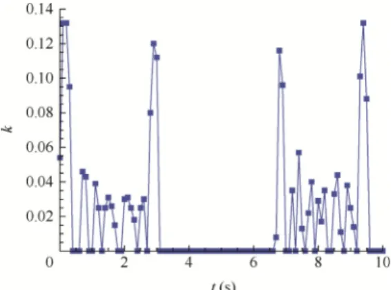
The parameter of reduced frequencykis employed as one of the input variables in most of the previous researches on intelligent modeling such as FL13–15and NNs.18For example, Ref.13took (a,a_,€a;k,b,de) as the input variables when mod-eling aerodynamics of pitching oscillations, while Ref.14took (a,/,/_,k,b,w,w_) as the input variables when modeling aero-dynamics of yawing and rolling oscillations, whereais angle of attack,bis sideslip angle,/is roll angle,deis elevator deflec-tion angle andwis yawing angle. It is noted that the reduced frequency is an unsteadiness parameter adopted specifically in forced-oscillation wind tunnel tests, which does not exist in flight tests. When the aerodynamic models set up from wind tunnel test data are used to predict aerodynamic characteristics in flight tests, an equivalent reduced frequency is needed, which is obtained by fitting a segment of flight test data. For example, the equivalent reduced frequency of pitching motion is calculated by solving an optimization problem15:
min a0;as;k;u J¼X n i¼1 fa ½a0þascosðksþuÞg 2 þX n i¼1 f_a ½asksinðksþuÞg 2 ð17Þ where_ais nondimensional rate of angle of attack;sis nondi-mensional time;nis the pre-specified number of points for fit-ting. The mean angle-of-attack a0, amplitude as, reduced frequencyk, and phaseuare the parameters to be determined. A series of problems arise from this processing technique: (a) The nonlinearity of the goal function may lead to local optimality. (b) Singularity may occur in some cases. As a spe-cial case,kcan be any value at constant angles of attack. (c) For coupled 6-DOF motions, it is not assured whether the equivalent reduced frequency should be determined in three directions of body-axis or in two directions of angle of attack and sideslip angle. (d) The number of points for fitting may have great effects on the resulting equivalent reduced fre-quency. (e) The resulting equivalent reduced frequency may vary acutely along with time. Fig. 3shows the time history of the equivalent parameter during a coupled yawing-rolling ramp motion.18 It skips frequently in the process of ramp
(0–3 s) and the reverse (6.7–9.7 s).
As a solution, several sampling points of the current and previous flight states could be employed to describe the effects of motion history. Ref.16took [a(s),a(s1),a(s2);a_(s),a_ (s1),a_ (s2);. . .] as input variables when modeling the longitudinal aerodynamics of a pitching delta wing by use of back propagation neural network (BPNN). Ref.19 took
[a(s),a(sDs),a(s2Ds),a(s3Ds),a(s4Ds);b(s), Fig. 2 LS-SVM modeling results of a two-dimensional nonlinear
b(sDs),b(s2Ds),b(s3Ds),b(s4Ds)] as input vari-ables when modeling 6-component aerodynamic coefficients by use of radius base function neural network (RBFNN). The references exhibit satisfying results.
In this way, however, two problems remain to be solved: (a) How long time before do the flight states have no effect upon the current aerodynamics? (b) How to determine the number of sampling points? As for the first question, the time length mÆDscan be determined according to the state-space models5,6 or the differential-equation models,7–10 to be (1–2) s
1 for instance, where s1 is the characteristic time constant in the mathematical models. As for the second question, the number of sampling pointsmcan be determined appropriately accord-ing to the above time length and the mode frequencies of the aircraft, to be [8(mÆDs)Æmax(xSP, xDR)] for instance, where
xSP is the nondimensional frequency of short-period mode andxDRis that of Dutch roll mode.
3.2. Selection of output variables
In intelligent modeling of high angle-of-attack unsteady aero-dynamics, the most direct output variables are aerodynamic force and moment coefficients. There is a fall in this way that the errors in dynamic test data will affect the predictions of sta-tic aerodynamics. As we know, dynamic wind tunnel test data include greater errors than static ones in general.
With a view to engineering application, aerodynamics can be decomposed as follows (pitch moment coefficient Cm as an example).
Cm¼Cm;stþDCm;dyn ð18Þ
A candidate way is to model the dynamic increment DCm,dyn instead of the aerodynamic coefficientCm, while the static componentCm,sttakes the static wind tunnel test results. Thus, all the dynamic test data, measured in different forms of motions and even in different wind tunnels, can be put together for SVM training.
3.3. Determination of SVM parameters
The selection of kernel function and determination of SVM parameters are another important problems for aerodynamic modeling. They also have decisive effects upon the fitting
precision, the generalization ability, and the training speed of SVMs.
The kernel function decides the mapping pattern from the input space to the feature space. Theoretically, the kernel can be any symmetry function satisfying Mercer’s condition. The commonly used kernels include:
(1) Polynomial function:K(x,xi) = (xTxi+ 1)q
(2) Radius base function (RBF):K(x,xi) = exp[||xxi||2/ (2r2)]
(3) Sigmoid function:K(x,xi) = tanh[r(xT-xi) +c] (4) Potential function:K(x,xi) = exp[||xxi||/(2r2)]
There is no universal principle to guide the selection of ker-nel function. However, the RBF kerker-nel is efficient for nonlin-ear system modeling, which is validated by a large number of simulation experiments and applications.
Having selected the kernel function (RBF kernel is adopted in unsteady aerodynamic modeling in the next section), the penalty factorcand the kernel widthrin LS-SVMs need also to be determined. The performance of LS-SVMs will be improved by adjusting the two parameters. The methods such asm-fold cross-validation and leave-one-out (LOO) can be uti-lized to determine these parameters.35,36
The m-fold cross-validation is the most commonly used method to estimate the generalization error. In this method, the training sample set is first partitioned intomsubsets with nearly the same size which do not intersect each other. For given parametersc andr, one of the subsets is taken as the testing set at a time, the others as the training set. After the parametersai(i= 1,2,. . .,n) andbin the model are obtained by the training algorithm from the training set, the mean square sum of prediction errors MSSEican be calculated for the testing set and is taken as the testing error. The average ofmtesting errors MSSE = (1/m)RMSSEiis taken as the gen-eralization error. Thus, the parameterscandrcan be adjusted according to the generalization error.
For a group of parameterscandr, totallymtimes of train-ing and testtrain-ing are needed to calculate the average error MSSE. Consequently, usingm-fold cross-validation to opti-mize the parameters is computationally expensive. The higher mis, the more computation time it costs. One should select an appropriate low value ofmto performm-fold cross-validation, especially in case of large number of training samples.
For unsteady aerodynamic modeling at high angles of attack, it is important that all the data of an individual dynamic test should be taken as a unit and put into same a subset during them-fold partitioning.
4. Results and discussion
4.1. Aerodynamic modeling of a pitching delta wing
The wind tunnel test data are taken from Ref.37The test model is a sharp-edged delta wing with aspect ratioA= 2, as shown inFig. 4. The pitching axis is located at 67%c0, wherec0is the
wing chord at midspan. The large-amplitude pitching
oscillation tests were carried out in the 7 foot·10 foot (1 foot = 30.48 cm) low-speed wind tunnel at NASA Ames Research Center, with Reynolds number Re= 4.5·105 and the pitch moment reference point at 77%c0.
Fig. 3 Equivalent reduced frequency of coupled yawing-rolling ramp motion.18
In the forced-oscillations, the time history of angle of attack is
aðsÞ ¼4545cosðksÞ ð19Þ
wherek=xc=Vis reduced frequency,cis mean aerodynamic chord,xis oscillation frequency,Vis velocity;s=tðV=cÞis nondimensional time. The nondimensional parameter charac-terizing unsteadinessK= 0.01, 0.02, 0.03, and 0.04, whereK is defined as
K¼a_maxc0=ð2VÞ ð20Þ
Converted to the conventional reduced frequency,k= 0.017, 0.034, 0.051, 0.068.
Fig. 4 The delta wing model with aspect ratioA= 2.
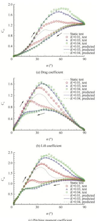
Fig. 5 LS-SVM predictions and training data of pitching delta wing.
Fig. 6 LS-SVM generalization and wind tunnel test data of pitching delta wing.
The unsteady aerodynamic data are transformed to the dynamic increments: CL;dyn¼CLCL;st DCD;dyn¼CDCD;st DCm;dyn¼CmCm;st 8 > < > : ð21Þ
At first, the LS-SVM models of DCL,dyn, DCD,dyn, and DCm,dynare set up respectively from the dynamic measurement data withK= 0.01, 0.03, 0.04, with RBF kernel adopted, and the input variables taken as a (s), a (s8), a (s16),
a (s24), a(s32), and q(s), where qis nondimensional pitching rate. This means that the instantaneous aerodynamics Cm(s), for example, depends upon the angle-of-attack history during [s32,s].
The SVM parameters determined by the m-fold cross-validation are listed as follows (with the sample inputs normalized):
CD: c¼3:2;2r2¼0:22 CL: c¼3:2;2r2¼0:21 Cm: c¼3:2;2r2¼0:22
Fig. 5shows the aerodynamic coefficients predicted by the LS-SVM models, in comparison with the measurement results, where the black dashed lines denote the static wind tunnel test data, the colored symbols are the dynamic wind tunnel test data, the colored lines are the predictions of the LS-SVM mod-els, and the arrows indicate the direction of hysteretic loops. The predictions approximate the wind tunnel test data well, which indicates that the LS-SVMs have great learning ability. Subsequently, the LS-SVM models are utilized to predict the aerodynamic characteristics of the large-amplitude pitch-ing oscillation withK= 0.02.Fig. 6shows the predicted aero-dynamics in comparison with that obtained by wind tunnel tests. The predictions are in agreement with the test data, in spite of some tolerable discrepancies, which shows that the LS-SVMs have satisfying generalization performance.
4.2. Aerodynamic modeling of a rolling aircraft configuration Ref.25presented the rolling oscillation wind tunnel test results
of F-16XL. The tests were executed with a 0.18-scale F-16XL model using a forced-oscillation rig in the 14 foot·22 foot subsonic wind tunnel at NASA Langley Research Center.
The test model was forced to roll around the longitudinal axis at the given pitch angles:/=/ssin(ks). Here, the reduced
fre-quency k¼xb0=ð2VÞ, the nondimensional time
s¼tð2V=b0Þ;b0is wing span.
In rolling oscillations, the angle of attack and sideslip angle vary as follows.
aðsÞ ¼tan1ðtanhcos/Þ
bðsÞ ¼sin1ðsinhsin/Þ
ð22Þ wherehis the pitch angle and/the roll angle.
The roll moment data were obtained at a series of pitching angles,h= 0, 10, 15, 20, 25, 30, 36, 40, 50, 60, 70, and 75, with the amplitude/s= 10, 20, and 30, and a con-stant maximum roll rate ofpmax¼pmaxb0=ð2VÞ ¼0:04.
The wind tunnel (W.T.) data used here are obtained from digitizing the AIAA paper. The error of roll moment coeffi-cientClin the data points is less than 0.0005.
Aerodynamic modeling is performed directly for the roll moment coefficient due to lack of the corresponding static test data. At first, the test data with/s= 10and 30are employed
to train the LS-SVM model of Cl, where RBF kernel is adopted also, and the input variables take a (s), a (s5),
a(s10),a(s15),a(s20),b (s), b(s5),b (s10),
b (s15),b(s20), andp(s). The SVM parameters deter-mined by m-fold cross-validation are (with the sample inputs normalized):c= 5.0 and 2r2= 0.58. The roll moment coeffi-cient predicted by the LS-SVM model, as well as the one obtained from wind tunnel measurement, is presented in Fig. 7, where the red circles are the dynamic wind tunnel test data, the blue solid lines denote the predictions of the LS-SVM model, and the arrows indicate the direction of hys-teretic loops. The figure shows a satisfactory approximation.
The LS-SVM model is then employed to predict the aerody-namic response to the rolling oscillations with the amplitude
/s= 20. Fig. 8 shows the predictions in comparison with the wind tunnel test data. It can be seen that there are some tolerable discrepancies in the range of a0= 30–50, where the unsteady aerodynamic effects are extremely great. Nevertheless, the overall agreement indicates the satisfying generalization performance of LS-SVMs.
5. Conclusions
SVMs are a novel type of machine learning method developed on the basis of statistical learning theory, embodying the struc-tural risk minimization principle. They are gaining popularity due to the features such as simple structure, global optimality and empirical performance. The following can be concluded from the presentations and applications in this paper.
(1) The aerodynamic modeling results of the pitching delta wing and the rolling aircraft configuration show that the LS-SVMs have excellent learning capability and sat-isfying generalization performance, and thus become an attractive means in the field of high angle-of-attack unsteady aerodynamic modeling.
(2) In order to describe the effects of motion history on aerodynamics, one can take several sampling points of the current and previous flight states as the inputs of SVMs. It is suggested to model the dynamic increments instead of aerodynamic coefficients, for the static wind tunnel test data have higher precision than dynamic ones in general.
(3) RBF kernel is an appropriate selection for unsteady aerodynamic modeling at high angles of attack. The penalty factor c and the kernel width r can be deter-mined by means ofm-fold cross-validation. It is impor-tant that all the data of an individual dynamic test should be taken as a unit and put into same a subset dur-ing them-fold partitioning.
Acknowledgments
The authors are grateful to all the members of their work group for help in the present research. They also thank the anonymous reviewers for their constructive review of the
manuscript. This study was supported by a Chinese
Government Contract.
References
1. Lin GF, Lan CE. A generalized dynamic aerodynamic coefficient model for flight dynamics applications. Reston: AIAA; 1997. Report No.: AIAA-1997-3643.
2. Tobak M, Schiff LB. Aerodynamic mathematical modeling-basic concepts. Moffett Field, CA:NASA Ames Research Center; 1981. Report No.: 19810022564.
3. Chin S, Lan CE. Fourier functional analysis for unsteady aerodynamic modeling.AIAA J1992;30(9):2259–66.
4. Murphy PC, Klein V. Estimation of aircraft nonlinear unsteady parameters from dynamic wind tunnel testing. Reston: AIAA; 2001. Report No.: AIAA-2001-4016.
5. Goman M, Khrabrov A. State-space representation of aerody-namic characteristics of an aircraft at high angles of attack. J Aircraft1994;31(5):1109–15.
6. Lutze FH, Fan YG, Stagg G. Multi-axis unsteady aerodynamic characteristics of an aircraft. Reston: AIAA; 1999. Report No.: AIAA-1999-4011.
7. Abramov NB, Goman MG, Khrabrov AN. Aircraft dynamics at high incidence flight with account of unsteady aerodynamic effects. Reston: AIAA; 2004. Report No.: AIAA-2004-5274. 8. Abramov N, Goman M, Demenkov M, Khrabrov A.
Lateral-directional aircraft dynamics at high incidence flight with account
of unsteady aerodynamic effects. Reston: AIAA; 2005. Report No.: AIAA-2005-6331.
9. Wang Q, Cai JS. Unsteady aerodynamic modeling and identifica-tion of airplane at high angles of attack.Acta Aeronaut Astronaut Sin1996;17(4):391–8 Chinese.
10. Wang Q, He KF, Qian W, Mao ZJ. Aerodynamic modeling of spatial maneuvering aircraft at high angles of attack. Acta Aeronaut Astronaut Sin2004;25(5):447–51 Chinese.
11. Huang XZ. Nonlinear indicial response/internal state-space rep-resentation and its application on delta wing aerodynamics. Reston: AIAA; 2003. Report No.: AIAA-2003-3944.
12. Pashilkar AA. Flight dynamic analysis of the flow incidence rate model. Reston: AIAA; 2002. Report No.: AIAA-2002-0098. 13. Wang Z, Lan CE, Brandon JM. Fuzzy logic modeling of nonlinear
unsteady aerodynamics. Reston: AIAA; 1998. Report No.: AIAA-1998-4351.
14. Wang Z, Lan CE, Brandon JM. Fuzzy logic modeling of lateral-directional unsteady aerodynamics. Reston: AIAA; 1999. Report No.: AIAA-1999-4012.
15. Wang Z, Lan CE. Unsteady aerodynamic effects on the flight characteristics of an F-16XL configuration. Reston: AIAA; 2000. Report No.: AIAA-2000-3901.
16. Rokhsaz K, Steck JE. Application of artificial neural networks in nonlinear aerodynamics and aircraft design. J Aerospace 1993;102:1790–8.
17. Soltani MR, Sadati N, Davari AR. Neural network: a new prediction tool for estimating the aerodynamic behavior of a pitching delta wing. Reston: AIAA; 2003. Report No.: AIAA-2003-3793.
18. Shi ZW, Wang ZH, Li JC. The research of RBFNN in modeling of nonlinear unsteady aerodynamics.Acta Aerodyn Sin2012;30(1): 108–12 Chinese.
19. Wang Q, He KF, Qian WQ, Zhang TJ, Cheng YQ. Unsteady aerodynamics modeling for flight dynamics application. Acta Mech Sin2012;28(1):14–23.
20. Wang Q, Wu KY, Zhang TJ, Kong YN, Qian WQ. Aerodynamic modeling and parameter estimation from the QAR data of an airplane approaching a high-altitude airport. Chin J Aeronaut 2012;25(3):361–71.
21. Singh R, Baeder J. Direct calculation of three-dimensional indicial lift response using computational fluid dynamics. J Aircraft 1997;34(4):465–71.
22. Ghoreyshi M, Cummings RM, DaRonch A, Badcock KJ. Transonic aerodynamic load modeling of X-31 aircraft pitching motions.AIAA J2013;51(10):2447–64.
23. Ghoreyshi M, Jirasek A, Cummings RM. Reduced order unsteady aerodynamic modeling for stability and control analysis using computational fluid dynamics.Prog Aerosp Sci2014;71:167–217. 24. Cooperative programme on dynamic wind tunnel experiment for
manoeuvering aircraft. Reston: AIAA; 1996. Report No.: AGARD-AR-305.
25. Brandon JM, Foster JV. Recent dynamic measurements and considerations for aerodynamic modeling of fighter airplane configurations. Reston: AIAA; 1998. Report No.: AIAA-1998-4447.
26. Huang D. Unsteady aerodynamic characteristics for the aircraft oscillation in large amplitude [dissertation]. Nanjing: Nanjing University of Aeronautics and Astronautics; 2007 [Chinese]. 27. Findlay D, Guruswamy G. Numerical analysis of aircraft high
angle of attack unsteady flows. Reston: AIAA; 2000. Report No.: AIAA-2000-1946.
28. Schu¨tte A, Einarsson G, Raichle A, Schoning B, Mo¨nnich W, Forkert T. Numerical simulation of manoeuvreing aircraft by aerodynamic, flight mechanics, and structural mechanics coupling. J Aircraft2009;46(1):53–64.
29. Paul R, Murua J, Gopalarathnam A. Unsteady and post-stall aerodynamic modeling for flight dynamics simulation. Reston: AIAA; 2014. Report No.: AIAA-2014-0729.
30. Gunn SR. Support vector machines for classification and regres-sion. Southampton (UK): University of Southampton; 1998. Report No.: ISIS-1-98.
31. Scho¨lkopf B, Sung K-K, Burges CJC, Girosi F, Niyogi P, Poggio T, et al. Comparing support vector machines with Gaussian kernels to radial basis function classifiers. IEEE Trans Signal Process1997;45(11):2758–65.
32. Fan H-Y, Dulikravich GS, Han Z-X. Aerodynamic data modeling using support vector machines. Reston: AIAA; 2004. Report No.: AIAA-2004-0280.
33. Vapnik V. The nature of statistical learning theory. New York: Springer-Verlag; 1995.
34. Suykens JAK, Vandewalle J. Least squares support vector machine classifiers.Neural Processing Letters1999;9(3):293–300. 35. Chapelle O, Vapnik V, Bousqet O, Mukherjee S. Choosing
multiple parameters support vector machines.Machine Learning 2002;46(1):131–60.
36. Deng NY, Tian YJ.A new method for data mining: support vector machines. Beijing: Science Press; 2004, p. 355-66 Chinese. 37. Jarrah MA, Ashley H. Impact of unsteadiness on maneuvers and
loads of agile aircraft. Reston: AIAA; 1989. Report No.: AIAA-1989-1282-CP.
Wang Qing is a researcher at the State Key Laboratory of Aerodynamics, as well as the Computational Aerodynamics Institute, China Aerodynamics Research and Development Center. He received the Ph.D. degree in flight dynamics from Northwestern Polytechnical University in 1995. His main research interests are system identifica-tion, flight dynamics, and unsteady aerodynamics.
Qian Weiqi is a researcher and Ph.D. supervisor at the State Key Laboratory of Aerodynamics, as well as the Computational Aerodynamics Institute, China Aerodynamics Research and Development Center. He received the Ph.D. degree in flight dynamics from Northwestern Polytechnical University in 1999. His current research interests are aerodynamic/aero-thermodynamic parameter estimation, aerodynamic data correlation and data fusion.
He Kaifeng is a researcher and Ph.D. supervisor at the State Key Laboratory of Aerodynamics, as well as the Computational Aerodynamics Institute, China Aerodynamics Research and Development Center. He received the Ph.D. degree in aircraft design from Northwestern Polytechnical University in 2008. His area of research includes flight dynamics, aerodynamics and subscaled model flight test techniques.
![Fig. 1 shows the topologic structure of SVMs. In Fig. 1, x = [x 1 , x 2 , . . ., x m ] T .](https://thumb-us.123doks.com/thumbv2/123dok_us/471240.2555646/3.892.453.814.82.447/fig-shows-topologic-structure-svms-fig-x-t.webp)