1948
APPLICATIONS OF MACHINE LEARNING ALGORITHMS
TO THE PROBLEM OF DETECTING UNKNOWN DATA
1AKHMER YERASSYL, 2AKHMER YERMEK, 3BEKTEMYSSOVA GULNARA
UMITKULOVNA, 4USKENBAYEVA RAISA KABIEVNA
1, 2, 3, 4Faculty of Information Technology, Department «Computer Engineering and Telecommunication»,
International Information Technology University, Almaty, Kazakhstan
E-mail: 1[email protected] , 2[email protected] , 3[email protected] 4[email protected],
ABSTRACT
Nowadays, the term big data means the work with large volumes and diverse composition, very often updated and located in different sources in order to increase work efficiency, create new products and increase. The problem of understanding a large number of unstructured and previously unknown data for the task is usually manually solved by a team of mathematicians and analysts who find it difficult to retain the value of all the data and all the hidden relationships of the incoming multidimensional array. However, in order to classify data, a full understanding of it is required. Today, there can be a lot of data sources: data from sensors of critical equipment (“Internet of things”), transactional “tires” and databases, electronic documents and paper media. In this regard, the quality of classifiers of most of the studying models decreases significantly. This article describes various machine learning methods for the classification of previously unknown data and ways to improve the quality of models. The advantages and disadvantages for each of the models are described, as well as the necessary and sufficient conditions for use. As experimental data, the Otto Product Classification dataset were taken from the open database.
Keywords: Machine Learning, E-Commerce, Classification, Decision Trees
1. INTRODUCTION
Today there are a large number of classes of business problems that are technically solved using machine learning algorithms. Machine learning algorithms are used in all areas such as e-retail, online banking, e-commerce, internet acquiring, the mining and smelting complex, and the oil and gas industry also have this problem. This is mainly due to the fact that the organizations create huge amounts of data, and the fact that most of them are presented in a format that does not correspond well to the traditional structured database format, those are web logs, videotapes, text documents, computer code or, for example, geospatial data. All this is stored in a variety of different repositories, sometimes even outside the organization. As a result, corporations may have access to a huge amount of their data and may not have the necessary tools to establish relationships between these data and draw significant conclusions from them. There are a large number of patterns that can be detected by analyzing data using data
analysis tools and predicting the most likely behavior, for example, the probability of a purchase or the detection of abnormal behavior, the presence of fraudulent and erroneous transactions. In the modern world, the sample data that is required to solve a specific task of searching a data structure does not have a standard format, and a lot of resources may be required for their qualitative analysis and classification. Often, sample data may be required from more than one source; accordingly, there is the problem of combining data and bringing it to a common standard.
1949 The relevance of the study lies in the identification and use of knowledge about cause-effect relationships, abstract knowledge and ideas of structured data, based on the application of basic statistical elements and probabilistic models. For example, the Otto Group is one of the world's largest e-commerce companies, which sells millions of products worldwide each day, adding several thousand products to our product line. The constant analysis of the effectiveness of the products is essential. However, due to the diverse global infrastructure, many absolutely identical products are classified differently. Thus, the quality of analysis of our products largely depends on the ability to accurately group similar products. The better the classification, the more information we can get about our range. Most often, the Information Cataloging System accepts data in its format and the process of transforming data from the source format to the format of a specific industry is a very expensive task that does not scale manually. On the other hand, the product catalog contains hidden information about the relationships between entities, types and values of properties of entities, abstract models and properties specific to each format, which can be used to create a predictive structure detection model from a previously unknown catalog. Thus, it becomes possible to automate the process of transforming data from one format to another, which will significantly increase its supplier base and product catalog.
2. RELATED WORK
This section has some related work that uses machine learning techniques inside of e-commerce and online store websites, and investigation of neural networks.
The ecosystem of modern business cannot develop without the introduction of information technology. This provision becomes particularly relevant in the field of trade. The sale of goods using the online store is applicable to businesses of any level, so the development of new methods that contribute to the successful interaction of classical trade and modern technology is undoubtedly relevant. The English scientist P.Flach argues that the point in using special machine learning algorithms is to “use the necessary attributes to build models that are suitable for solving the problems posed” [1]. At the same time, “models provide a variety of machine learning subject, while tasks and signs give it unity” [2].
By e-commerce, A. Yurasov, understands as “any kind of transactions in which the interaction of the parties is carried out electronically instead of physical exchange or direct physical contact [1]. With regard to modern realities, this includes, first of all, buying and selling via the Internet, which requires a careful individual approach to customers at all stages: from promotion of a site or a specific product to expanding the range of consumer demand and improving the system of ordering and receiving orders, as well as feedback [3]. That is the reason, why machine learning in this area becomes especially necessary. One of the modern methods of presenting goods to a client, described in the work was a recommendation list of goods, based on the study of his previous purchases and searches [4]. The model of recommendations is very popular and widely used in big companies such as Amazon and Alibaba. It is a business model, which helps to attract customers and drive revenue. The current work is dedicated to recognizing unknown products based on the previous data, and it can be considered as an initial step in the chain processes of e-commerce companies. This step is very important and it is directed to saving time and resources for identifying products.
Analysis of audio and video data, was proposed by N. Bauman, M. Volosatova and V. Yablokov researchers of MGTU. The analysis allows analyzing the specific behavior of the visitors of the store by studying the data of the tracking system. This allows you to optimize the trading process and make it more customer-oriented. Thanks to the introduction of machine learning, it is possible to take into account such parameters as the number of visitors, the calculation of time spent at the point of sale [5].
1950
3. THEORETICAL REVIEW OF MACHINE
LEARNING ALGORITHMS IN THE CLASSIFICATION PROBLEM
This section is devoted to describe machine learning techniques in the classification problem. Classification is one of the sections of machine learning, dedicated to solving the following problem. There are many “objects” that are divided in some way into “classes”. A finite set of objects is given for which it is known which classes they belong to. This set is called the "training set". Class affiliation of other objects is not known. It is required to construct an algorithm capable of classifying an arbitrary object from the original set [7][8]. In machine learning, the task of classification relates to the training section with the teacher. There is also training without a teacher, when the division of objects of the training sample into classes is not specified, and it is required to classify objects only on the basis of their similarity to each other. In this case, it is customary to talk about clustering or taxonomy problems, and the classes are called clusters or taxons, respectively. In some applied areas, and even in mathematical statistics itself, there is a tendency to call clustering problems classification problems.
The main algorithms such as logistic regression, support vector machines, neural networks, decision trees, random forest, gradient boosting were considered.
3.1 Logistic regression
Logistic regression is a type of multiple regressions, the general purpose of which is to analyze the relationship between several independent variables and the dependent variable. Binary logistic regression applies when the dependent variable is binary. In other words, using the logistic regression, it is possible to estimate the probability that an event will occur for a specific subject [7].
To solve the problem, the regression problem can be formulated as follows: instead of predicting a binary variable, we predict a continuous variable with values on the interval [0,1] for any values of independent variables. This is achieved by applying the following regression equation, a logit transform:
y
e
p
1
1
(1)
Where
p
-is the probability, that event will happen, andy
-standard equation of regression [8].Suppose that we discuss about our dependent variable in terms of the basic probability
p
, which lies between 0 and 1. Then we transform this probabilityp
:)
1
(
log
'
P
P
P
e
[image:3.612.313.521.151.343.2](2)
Figure 1: Plot of logistic regression
There are many ways of finding linear regression coefficients. One of the popular methods is the maximum likelihood method. We will give main advantages and disadvantage of this algorithm.
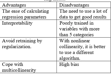
Table 1: Advantages And Disadvantages Of Logistic Regression.
Advantages Disadvantages
The ease of calculating
regression parameters The need to use a lot of data to get good results Interpretability Poorly trained in
variables with more than 5 categories Avoid retraining by
regularization.
With nonlinear collinearity, it is better to use a different algorithm. Cope with
multicollinearity
High bias
3.2 Decision trees
[image:3.612.309.528.452.598.2]1951
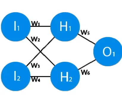
Figure 2: Example of decision trees
Here is an example of a binary decision
tree. As we can see, linear models do not reflect the peculiarities of the decision-making process in humans. In fact, when a person wants to understand this or that thing, he will ask a sequence of simple questions that will eventually lead him to some kind of answer [9]. Conditions in the inner vertices are selected extremely simple. The most frequent option is to check if the value of a certain attribute
j
[image:4.612.85.530.352.708.2]x
lies to the left than the specified thresholdt
:x
j
t
(3)Table 2: Advantages And Disadvantages Of Decision Trees.
Advantages Disadvantages
It is easily interpreted when a tree contains several levels.
Prone to overfitting
Easily cope with many categorical variables
Possible problems with diagonal solutions. Works well with
decision boundaries. Can be violated by small variations It can be visualized
Requires a little data preparation
Able to cope with multiple outputs Able to validate a model using statistical tests. That makes it possible to account for the reliability of the model.
3.3 Bayesian approximation.
Let some object have a feature vector
x
. It is necessary to determine which classy
this object belongs to. The Bayesian classifiera
(x
)
relates an object to such a class, the probability of which, provided that the object is realized, is maximal [10]:
) ( ) | ( max arg
) | ( max arg ) (
y P y x P
x y P x
a
y y
(4)
According to the Bayes theorem:
P
(
y
|
x
)
P
(
x
|
y
)
P
(
y
)
/
P
(
x
)
(5)The naive Bayes classifier solves the problem of data shortage [10]. With this problem, restoring density as a function of all the signs remains rather difficult. Distribution density signs in the product of densities for each attribute:
)
|
(
...
)...
|
(
)
|
(
)
|
(
) (
) 1 ( )
1 (
y
x
P
y
x
P
y
x
P
y
x
P
N
(6)
Where
x
k
k
is the sign of the objectx
. This hypothesis is fulfilled only if the signs are independent. This is by no means always the case, but with some degree of accuracy this approximation can be used.[15)Table 3: Advantages And Disadvantages Of Bayes Approximation.
Advantages Disadvantages
It is easily interpreted when a tree contains several levels.
Strongly depends on independence property of attributes, the quality of the model is greatly deteriorated if this condition is not present. Easy to calculate
Works well on high dimensions
3.4 Neural Networks.
In classification problems, the target variable
y
takes a finite set of values and is called a class label. Let li i
i
y
x
,
}
01952
d
i
R
x
andy
i
{
1
;
1
}
be the attributedescription and class label for the
i
th object, respectively. It is required to build a dividing surface:
a
(
x
)
y
{
1
,
1
}
(7)Which separates objects of one class from objects of another class in such a way that, if
a
(
x
)
0
,
then the object
x
belongs to the classy
1
, and, ifa
(
x
)
0
, thenx
it belongs to the class1
y
. [image:5.612.320.525.116.280.2]A neuron is a computational unit that receives information, performs simple calculations on it, and passes it on [11]. They are divided into three main types: input (blue), hidden (red) and output (green). There is also a displacement neuron. In the case when the neural network consists of a large number of neurons, the term layer is introduced. Accordingly, there is an input layer that receives information from hidden layers (usually no more than 3 of them) that process it and an output layer that displays the result [12]. Each of the neurons has 2 main parameters: input data output. In the case of an input neuron: input = output. In the others, the input information contains the total information of all neurons from the previous layer, after which it is normalized using the activation function
f
(
x
)
. A synapse is a connection between two neurons. The synapses have only one parameter, it is weight. So the input information changes when it is transmitted from one neuron to another [13]. The activation function is a way to normalize the input data. That is, if you have a large number at the input, by passing it through the activation function; you will get the output in the desired interval.Figure 3: Example of neural networks
Figure 3 shows example of neural networks. All nodes are neurons, and lines between them are synapsis.
Table 4: Advantages And Disadvantages Of Neural Networks.
Advantages Disadvantages
There is no need to formalize knowledge, formalization is replaced by example training
The difficulty of verbalizing the results of the neural network and explaining why it made a decision;
The possibility of processing multidimensional (dimension more than three) data and knowledge without increasing labor intensity
The inability to guarantee repeatability and
uniqueness of the results.
They can handle noise or conflicting data very well
The fault tolerance and survivability with the hardware
1953
3.5 Support Vector Machines.
Let, for simplicity, consider the problem of binary classification and some linearly separable sample. A sample is called linearly separable if there is a hyperplane in the feature space such that objects of different classes will be on different sides of this plane [14]. In this case, the hyperplane may not be carried out in a unique way, and the problem arises of finding the optimal separating hyperplane
w
,
x
w
0
0
. Let the separating hyperplane exist and is given by the equation.
a
(
x
)
sign
(
w
,
x
w
0)
(8)It is possible to choose two hyperplanes parallel to it and located on opposite sides of it so that there are no sample objects between them, and the distance between them is maximum [15]. In this case, each of the two resulting boundary planes will be “assigned” to the corresponding class.
L
(
M
i)
max{
0
,
1
M
i}
(
1
M
i)
(9)Of course, in some form you are already familiar with it. This is simply a linear classifier using a piecewise linear loss function and a
L
2-regulator:( ) || 2||
min
1 i w
l
i
w M
L
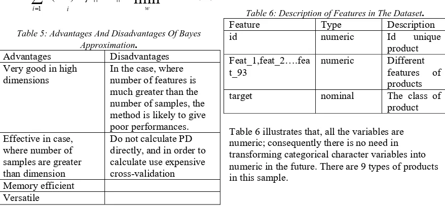
(10)Table 5: Advantages And Disadvantages Of Bayes Approximation.
Advantages Disadvantages
Very good in high dimensions
In the case, where number of features is much greater than the number of samples, the method is likely to give poor performances. Effective in case,
where number of samples are greater than dimension
Do not calculate PD directly, and in order to calculate use expensive cross-validation Memory efficient
Versatile
4. EXPERIMENTAL DATA
In this article, an e-commerce product was taken as experimental data, data from 93 variables and more than 200,000 products. All variables are numeric, representing the length, width, height, the average price, the number of purchases of certain product and so on. Therefore, you need to build a predictable model to determine the class for new products. Otto Group is one of the world's largest e-commerce companies. They sell millions of products daily around the world, adding several thousand products to our product line. The ongoing analysis of the effectiveness of our products is very important is. However, due to the diverse global infrastructure, many identical products are classified differently. Thus, the quality analysis of products largely depends on the ability to accurately group similar products. The better the classification, the more information you can get about the assortment. As a tool to analyze data and build predictive mathematical model was Python version 3.5. It has a lot of modern algorithms of machine learning.
[image:6.612.87.526.474.678.2]In order to figure out the model with relatively high accuracy, we will first use various models of classification training, including solving trees, Bayesian approaches, a neural network, and regression-based methods, random forest, decision trees. After that, we will compare the results of each model and choose the best of them.
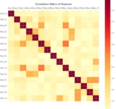
Table 6: Description of Features in The Dataset.
Feature Type Description
id numeric Id unique
product Feat_1,feat_2….fea
t_93
numeric Different features of products
target nominal The class of
product
1954
Figure 4: Distribution of classes in the dataset
As we can see in Figure 4 there is no equal distribution between classes, class 2 contains 25% of the whole product, class 1 has less than 5 % , and it is smallest on, comparing to others. We divided our dataset into two parts, 70% of dataset is training and 30% is test dataset. The training dataset has 61,878 rows, while the testing dataset has 144,368 rows.
Figure 5: Histogramm of training dataset.
Figure 5 illustrates distribution between 9 classes in the training dataset.
Our dataset is a 61878x94 matrix. Each column (except the last column) represents one feature and each row represents one product. The last column differs from one to nine for each row, in other words for each product, this is the variable, which we are going to predict, since we are doing supervised learning.
Note, the data points are described by their features already; we are directly in the setting of the feature space. We will give some statics on this data, and it will be our initial analysis. Since, we have 93 features; it would be cumbersome to enumerate all of their statistics. Hence we present only some relevant values to give an idea of each statistical collection.
TABLE 7:STATISTIC OF THE OTTO DATASET.
Mean Median Standard
deviation
Median 0,48 0 1,91
Max 2,89 1 5,78
Mean 0,02 0 0,21
For each of this statistic we create a new matrix with dimension 1x93, for each 93 features.
5. PROPOSED METHODOLOGY
The scheme for solving this problem is as follows.
1. Research analysis. In this step, we performed a one-dimensional and two-dimensional analysis of data, processing emissions, processing missing values. Missing values were replaced by averages. In this project, all data was in a numeric format, so converting from nominal variables to numeric variables was optional.
2. Correlation analysis. A correlation matrix was constructed with dimension 93x93for each class separately. Correlation analysis helps to get a preliminary idea into dataset. Pearson correlation coefficient was used to find linear relationships for each class separately; it can be seen in Figure 6. The colors indicate the strength of correlation between each feature. We see that the correlation in Figure 7 of a feature with itself is one, therefore the. The variables correlating over 50% were not included in the model.
3. Feature importance analysis. Top variables relevant for the model were selected.
4. Application of the above described algorithms for machine and deep learning.
[image:7.612.90.299.415.576.2]1955
Figure 6: Correlation Matrix between classes
Figure 7: Correlation Matrix between features
5.1 Logistic regression
We broke the problem into nine binomial regression problems. For each binomial regression problem, we tried to predict whether the certain product would fall into one class [7]. The stepwise feature selection is used to improve the strength of the models, and AIC test is used to select the best one. We then aggregated the probabilities of the nine classes, weighted by the deviance of these nine models, into one single final probability matrix. We came up to conclusion with this approach that is extremely time consuming [8]. Running one binomial regression model with stepwise feature selection could take up to an hour for the training set. The weights were assigned to the nine models, and it seemed to have a significant influence on the accuracy of the model. We can combine boosting
and resampling methods to get better scores, but the limited computational performance makes us to look for a faster and more capable alternative [5].
5.2 Decision trees
In this research we tried to go deeply into building tree based models. Firstly we started with building decision tress. One of our observations that decision trees are very susceptible to small changes in the data, which can lead to the generation of a new tree. Decision trees belong to heuristic algorithms, that is, at each node they reach a local minimum, which does not necessarily lead to a global minimum. Another thing to know, that the deeper the tree, the more complex the decision rules and the fitter the model.
In our problem, decision tree did not predict half of the classes, such as class_1, class_3, class_4, class_7. This was a common problem and sign of overfitting. So, we concluded, that basic decision trees are easy to understand, but as we experienced in their performance above, they might over fit, and can lose good signal easily, and have low practical performance.
We decided to start to look at more complex tree-based models that aim to correct those deficiencies by growing multiple trees and aggregating them together to make better accuracy, hence predictions. Bagging, or bootstrap aggregating, reduces the variance found in a single decision tree model by making multiple predictions for each observation and choosing the most commonly occurring response (or class in our case). Theoretically this should help us to reduce the over-fitting found in a basic decision tree model.
The best solutions for avoiding these problems were using random forest, because it is improvement of all bagging models [5].
5.3 Random forest
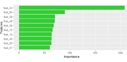
[image:8.612.96.296.296.484.2]1956 split step, specific random sample of all the features is taken. Out of all features, the strongest one is decided to split [16].
Figure 8: Importance features
Using random forest we are able to get top 10 features, according to their importance in the Figure 8.
The composition of
N
algorithms is the combination of algorithms into one)
(
),....,
(
1
x
b
x
b
N . The idea is to train thealgorithms
b
1(
x
),....,
b
N(
x
)
, and then average theresponses received:
Nn
n
x
b
N
x
a
1
).
(
1
)
(
(11)In our task, we applied the technique for classification, for this we need to get a sign from the received expression:
Nn
n
x
b
N
sign
x
a
1
).
(
1
)
(
(12)To build the composition, we used the bootstrap method, trained the basic algorithms on different subsamples of the training sample, since the decisive trees vary greatly from even small changes in the training sample, such randomization greatly increases the difference between the basic algorithms.
The algorithm used to build a random forest is following:
1. Constructed using bootstrap
N
randomsubsamples
X
``
nn
1
,...
N
.2. Each resulting subsample
`
`
nX
was used as a training sample to build the corresponding decision treeb
n(x
)
. And:• A tree is built until there are no more objects in each
n
minsheet .• The process of building a tree is randomized: at the stage of choosing the optimal feature, according to which the partition will occur, it is not searched for among the whole set of features, but among a random size
q
subset.• The random size
q
subset is selected again each time it is necessary to split the next vertex. This is the main difference between this approach and the method of random subspaces, where a random subset of features was selected once before building the basic algorithm [16].3. Built trees are combined into a composition. We recall the formula:
Nn
n
x
b
N
sign
x
a
1
).
(
1
)
(
(13)Random forest is a composition of deep trees that are built independently of each other. But this approach has the following problem. Teaching deep trees requires a lot of computational resources, especially in the case of a large sample or a large number of attributes. If we limit the depth of the decisive trees in a random forest, then they will no longer be able to capture complex patterns in the data. This will cause the shift to be too large. The second problem with a random forest is that the process of building trees is undirected: each next tree in the composition does not depend on the previous ones. Because of this, to solve complex problems requires a huge number of trees. These problems can be solved with the help of the so-called boosting. Boosting is an approach to the construction of compositions, in which:
• Basic algorithms are built sequentially, one after another.
• Each following algorithm is constructed in such a way as to correct the mistakes of an already constructed composition. Due to the fact that the construction of compositions in the boosting is directional, it is sufficient to use simple basic algorithms, such as shallow trees.
5.4 Gradient boosting
Description of the gradient boosting algorithm is following:
1. Initialization of the composition
)
(
)
(
00
x
b
x
a
, that is, the construction of a simple algorithmb
0.2. Iteration step:
1957
)))
(
,
(
'
)),
(
,
(
'
1 1 1 1 l n l z n zx
a
y
L
x
a
y
L
F
s
(14)
, where
L
(
y
,
z
)
- loss function,y
-true answer,z
- prediction of algorithm [5]. (b) An algorithm is constructed
n i m bn
b
x
l
x
b
1)
(
1
min
arg
)
(
(15)the parameters of which are chosen in such a way that its values on the elements of the training sample were as close as possible to the computed optimal shift vector
s
.(c) Algorithm
b
n(
x
)
added to composition
nm m
n
x
b
x
a
1
)
(
)
(
. (16)3. If the stopping criterion is not met, then perform one more iteration step. If the stop criterion is satisfied, stop the iteration process [16].
In practice, we faced with the problem, that the implementation of the gradient boosting is a very difficult task, in which success depends on many fine points. In this text, we will look at a specific implementation of gradient boosting - the XGBoost package in Python, which is considered one of the best to date. It is worth to mention about LGBM, which is more efficient and faster version.
XGBoost has a number of important features.
1. The basic algorithm approximates the direction calculated by taking into account the second derivatives of the loss function.
2. The deviation of the direction constructed by the basic algorithm is measured using a modified functional — the division by the second derivative is removed from it, thereby avoiding numerical problems.
3. Functional is regularized - penalties are added for the number of leaves and for rate coefficients. 4. When constructing a tree, an informativity criterion is used, depending from the optimal shift vector.
5. The stopping criterion for learning a tree also depends on the optimal shift.
XGBoost package provided a quick and accurate method for this project, eventually providing the best accuracy of all models attempted [6]. Cross validation was performed to identify appropriate tree depth and avoid
overfitting. Then, an xgboost model was trained
and applied the test set to score the accuracy.
6. OBTAINED RESULTS
6.1 Results on experimental data
Table 8: Algorithms and Their Accuracy.
Algortihms Accuracy
Random forest 75%
Decision tree 72%
Neural networks 71%
Vector support machine 74% Logistic regressioon 72% Gradient boosting
(xgboost) 83%
Naïve Bayes 71%
Random Forest often outperform normal decision tree, particularly in larger datasets because of its ensemble approach. The drawback being it is computationally expensive. Random forest was built at small number of trees 50, was computationally slow, and showed the average accuracy 75%. The gradient boosted trees model, in which decision trees were created sequentially to reduce the residual errors from the previous trees, performed quite well and at a reasonable speed. This model was implemented with ntrees =100 and the default learn rate of 0.1. Also we got neural networks showed less accuracy; the reason might be that Neural Networks are bad with sparse data.
Using Naïve Bayes we got 70% score. As we said earlier this result was expectable, because it assumes that member variables are independent of each other. In our dataset, there are some features with high correlation with other features. Consequently, low AUC (70%) is justified.
6.2 The difference form current literature
1958
7. CONCLUSION
As we can see from the table 8, we have achieved of best results using gradient boosting. There are many factors, such as data size and type, which have lots of influence on model performance. In general, model ensembling is a very powerful technique nowadays. It can be used in both classification and regression. All the techniques in the article are widely used by data scientists.
In this article, we reviewed several machine learning algorithms for the problem of classifying previously unknown products. This problem is very relevant, as companies all seek to automate processes, while reducing the level of elapsed time. A comparative analysis was made after each of the methods; the advantages and disadvantages of the machine and deep learning algorithms for our problem are presented. Experimental data were reviewed from data from the Otto group. During the study, all the necessary steps of data processing, cleaning, normalization and transformation were carried out. For the classification problem, the method of logistic regression, decision trees, random forest ensembles, SVM, neural networks and gradient boosting were used.
These approaches, given in the article might be very useful for e-commerce companies and also can be very good for getting inside of mathematic behind machine learning algorithms.
Further investigation might be done on automatization of this model, in the way there is no need for participation of a human. So the machine will know which algorithm best fits into the problem and apply it with expected output, classified products [17].
REFRENCES:
[1] A.Yurasov, “Century Electronic commerce”
Textbook. allowance. - M .: Business, 2003. -
480 p.
[2] P.Flach , “Machine learning. The science and art of building algorithms that extract knowledge from data”, DMK Press, 2015. -
400 p.
[3] J. Ben Schafer, A. Konstan, J.Riedl, "E-commerce recommendation applications", Applications of Data Mining to Electronic Commerce. Springer US, 2001. 115-153 p.
[4] J. Ben Schafer, A. Konstan, J.Riedl, “E-Commerce Recommendation Applications”, Data Mining and Knowledge Discovery,
Kluwer Academic Publishers, 115–153 p,
2001, Netherlands
[5] P. Domingos, “High algorithm, how machine learning will change our world”, Mann, Ivanov and Ferber, 2016. - 336 p.
[6] C. Bishop, “Pattern Recognition and Machine Learning”, Springer, 2006
[7] T.Hastie, R.Tibshirani, J.Friedman, “The Elements of Statistical Learning Data Mining, Inference, and Prediction”, Second Edition, Springer, 2017, 764p
[8] Hal Daumé III, “A Course in machine learning”, Copyright, First printing,
September 2015, 193 p
[9] L.Breiman., J.Friedman, C.Stone, R.A.Olshen,, “Classification and regression trees”. CRC press, 1984.
[10] D.Barber, “Bayesian Reasoning and Machine Learning”,Cambridge University Press, 2017
[11] I.Goodfellow, Y.Bengio and A.Courville, “Deep Learning”, An MIT Press book, 2007
[12] D.Michie, D.J.Spiegelhalter, C.C.Taylor, “Machine Learning, Neural and Statistical Classificationm”, (1) University of Strathclyde, (2) MRC Biostatistics Unit, 1994, 298 p.
[13] M.W.Sholom, N.Indurkhya, T.Zhang, F.J.Damarau, “Text minig. Predictive methods of analyzing unstructured information”, 2004. — 236
[14] C.Burges, “A tutorial on support vector machines for pattern recognition”. http://research.microsoft.com/ en-us/um/people/cburges/papers/SVMTutorial.pd f.
[15] L.Breiman, "Random forests." Machine learning, 2005, 5-32 p.
[16] Zhi-Hua Zhou, “Ensemble Methods: Foundations and Algorithms”, CRC Press,
2012, 212p.