Xinyang Yi [email protected]
Constantine Caramanis [email protected]
Department of Electrical and Computer Engineering, The University of Texas at Austin, Austin, TX 78712
Eric Price [email protected]
Department of Computer Science, The University of Texas at Austin, Austin, TX 78712
Abstract
Binary embedding is a nonlinear dimension re-duction methodology where high dimensional data are embedded into the Hamming cube while preserving the structure of the original space. Specifically, for an arbitrary N distinct points in Sp−1, our goal is to encode each point us-ing m-dimensional binary strings such that we can reconstruct their geodesic distance up to δ uniform distortion. Existing binary embed-ding algorithms either lack theoretical guaran-tees or suffer from running time O mp
. We make three contributions: (1) we establish a lower bound that shows any binary embedding oblivious to the set of points requires m = Ω(δ12logN)bits and a similar lower bound for
non-oblivious embeddings into Hamming dis-tance; (2) we propose a novel fast binary embed-ding algorithm with provably optimal bit com-plexity m = O δ12logN
and near linear run-ning timeO(plogp)whenever logN δ√p, with a slightly worse running time for larger logN; (3) we also provide an analytic result about embedding a general set of points K ⊆
Sp−1with even infinite size. Our theoretical find-ings are supported through experiments on both synthetic and real data sets.
1. Introduction
Low distortion embeddings that transform high-dimensional points to low-high-dimensional space have played an important role in dealing with storage, information re-trieval and machine learning problems for modern datasets. Perhaps one of the most famous results along these lines
Proceedings of the32nd International Conference on Machine Learning, Lille, France, 2015. JMLR: W&CP volume 37. Copy-right 2015 by the author(s).
is the Johnson-Lindenstrauss (JL) lemma Johnson & Lindenstrauss (1984), which shows that N points can be embedded into a O δ−2logN-dimensional space while preserving pairwise Euclidean distance up to δ-Lipschitz distortion. This δ−2 dependence has been shown to be
information-theoretically optimalAlon(2003). Significant work has focused on fast algorithms for computing the embeddings, e.g., (Ailon & Chazelle, 2006; Krahmer & Ward, 2011; Ailon & Liberty, 2013; Cheraghchi et al.,
2013;Nelson et al.,2014).
More recently, there has been a growing interest in design-ing binary codes for high dimensional points with low dis-tortion, i.e., embeddings into the binary cube (Weiss et al.,
2009;Raginsky & Lazebnik,2009;Salakhutdinov & Hin-ton,2009;Gong & Lazebnik,2011;Yu et al.,2014). Com-pared to JL embedding, embedding into the binary cube (also called binary embedding) has two advantages in prac-tice: (i) As each data point is represented by a binary code, the disk size for storing the entire dataset is reduced consid-erably. (ii) Distance in binary cube is some function of the Hamming distance, which can be computed quickly using computationally efficient bit-wise operators. As a conse-quence, binary embedding can be applied to a large number of domains such as biology, finance and computer vision where the data are usually high dimensional.
While most JL embeddings are linear maps, any binary em-bedding is fundamentally a nonlinear transformation. As we detail below, this nonlinearity poses significant new technical challenges for both upper and lower bounds. In particular, our understanding of the landscape is signifi-cantly less complete. To the best of our knowledge, lower bounds are not known; embedding algorithms for infinite sets have distortion-dependenceδ significantly exceeding their finite-set counterparts; and perhaps most significantly, there are no fast (near linear-time) embedding algorithms with strong performance guarantees. As we explain below, this paper contributes to each of these three areas. First, we detail some recent work and state of the art results.
Recent Work. A common approach pursued by several ex-isting works, considers the natural extension of JL embed-ding techniques via one bit quantization of the projections:
b(x) =sign(Ax), (1.1) wherex∈Rpis input data point,A∈Rm×pis a projec-tion matrix andb(x)is the embedded binary code. In par-ticular,Jacques et al.(2011) shows when each entry ofAis generated independently fromN(0,1), withm > δ12logN
it with high probability achieves at mostδ(additive) distor-tion forN points. Work inPlan & Vershynin(2014) ex-tend these results to arbitrary setsK ⊆ Sp−1 where|K| can be infinite. They prove that the embedding with δ -distortion can be obtained whenm & w(K)2/δ6 where
w(K)is the Gaussian Mean Widthof K. It is unknown whether the unusual δ−6 dependence is optimal or not.
Despite provable sample complexity guarantees, one bit quantization of random projection as in (1.1), suffers from
O mp
running time for a single point. This quadratic de-pendence can result in a prohibitive computational cost for high-dimensional data. Analogously to the developments in “fast” JL embeddings, there are several algorithms pro-posed to overcome this computational issue. Work inGong et al.(2013) proposes a bilinear projection method. By set-ting m = O(p), their method reduces the running time fromO(p2)toO(p1.5). More recently, work inYu et al.
(2014) introduces a circulant random projection algorithm that requires running time O plogp. While these algo-rithms have reduced running time, to the best of our knowl-edge, the measurement complexities of the two algorithms are still unknown. Another line of work considers learn-ing binary codes from data by solvlearn-ing certain optimiza-tion problems (Weiss et al., 2009;Salakhutdinov & Hin-ton,2009; Norouzi et al.,2012;Yu et al.,2014). Unfor-tunately, there is no known provable bits complexity result for these algorithms. It is also worth noting thatRaginsky & Lazebnik(2009) provide a binary code design for pre-serving shift-invariant kernels. Their method suffers from the same quadratic computational issue compared with the fully random Gaussian projection method.
Another related dimension reduction technique is locality sensitive hashing (LSH) where the goal is to compute a dis-crete data structure such that similar points are mapped into the same bucket with high probability (see, e.g.,Andoni & Indyk(2006)). The key difference is that LSH preserves short distances, but binary embedding preserves both short and far distances. For points that are far apart, LSH only cares that the hashings are different while binary embed-ding cares how different they are.
Contributions of this paper. In this paper, we address several unanswered problems about binary embedding:
1. We provide two lower bounds for binary embeddings.
The first shows that any method for embedding and for recovering a distance estimate from the embed-ded points that is independent of the data being em-bedded must useΩ(δ12logN)bits. This is based on
a bound on the communication complexity of Ham-ming distance used by (Jayram & Woodruff, 2013) for a lower bound on the “distributional” JL embed-ding. Separately, we give a lower bound for arbitrarily data-dependent methods that embed into (any func-tion of) the Hamming distance, showing such algo-rithms requirem= Ω( 1
δ2log (1/δ)logN). This bound
is similar toAlon(2003) which gets the same result for JL, but the binary embedding requires a different construction.
2. We provide the first provable fast algorithm with optimal measurement complexity O δ12logN
. The proposed algorithm has running time O δ12log
1
δlog
2
Nlogplog3logN+plogpthus has almost linear time complexity when logN . δ√p. Our algorithm is based on two key novel ideas. First, our similarity is based on the median Hamming distance of sub-blocks of the binary code; second, our new embedding takes advantage of apair-wise inde-pendence argument of Gaussian Toeplitz projection that could be of independent interest.
3. For arbitrary set K ⊆ Sp−1 and the fully random
Gaussian projection algorithm, we prove that m = O(w(K+)2/δ4)is sufficient to achieveδuniform
dis-tortion. HereK+ is anexpandedset ofK. Although
in general K ⊆ K+ and hence w(K) ≤ w(K+), for interestingKsuch as sparse or low rank sets, one can showw(K+) = Θ(w(K)) p. Therefore ap-plying our theory to these sets results in an improved dependence onδcompared to a recent result inPlan & Vershynin(2014). See Section3.3 for a detailed discussion.
Discussion. For the fast binary embedding, one sim-ple solution, to the best of our knowledge not previously stated, is to combine a Gaussian projection and the well known results about fast JL. In detail, consider the strategy
b(x) = sign(AFx), where A is a Gaussian matrix and Fis any fast JL construction such as subsampled Walsh-Hadamard matrix Rudelson & Vershynin (2008) or par-tial circulant matrix Krahmer et al. (2014) with column flips. A simple analysis shows that this approach achieves measurement complexity O(1
δ2logN) and running time
O(δ14 log 2
Nlogplog3logN +plogp)by following the best known fast JL results. Our fast binary embedding al-gorithm builds on this simple but effective thought. Instead of using a Gaussian matrix after the fast JL transform, we use a series of Gaussian Toeplitz matrices that have fast matrix vector multiplication. This novel construction
im-proves the running time byδ2while keeping measurement
complexity the same. In order for this to work, we need to change the estimator from straight Hamming distance to one based on the median of several Hamming distances. An interesting point of comparison is Ailon & Rauhut
(2014), which considers “RIP-optimal” distributions that give JL embeddings with optimal measurement complexity O(δ12 logN)and running timeO(plogp). They show the
existence of such embeddings wheneverlogN < δ2p1/2−γ for any constantγ >0, which is essentially no better than the bound given by the folklore method of composing a Gaussian projection with a subsampled Fourier matrix. In our binary setting, we show how to improve the region of optimality by a factor ofδ. It would be interesting to try and translate this result back to the JL setting.
Notations. We use[n]to denote set{1,2, . . . , n}. We use
xI to denote the sub-vector ofxwith index setI ⊆ [n]. We denote entry-wise vector multiplication as xy = (x1y1, x2y2, . . . , xnyn)>. For two random variablesX, Y,
we denote the statement thatX andY are independent as X⊥Y. For two binary strings a,b ∈ {0,1}m, we use dH(a,b)to denote the normalized Hamming distance, i.e., dH(a,b) :=m1 Pm
i=11(ai 6=bi).
2. Problem Setup and Preliminaries
In this section, we state our problem formally, give some key definitions and present a simple (known) algorithm that sets the stage for the main results of this paper.
2.1. Problem Setup
Given a set ofp-dimensional points, our goal is to find a transformationf : Rp 7→ {0,1}msuch that the Hamming distance (or other related, easily computable metric) be-tween two binary codes is close to their similarity in the original space. We consider points on the unit sphereSp−1 and use the normalized geodesic distance (occasionally, and somewhat misleadingly, called cosine similarity) as the input space similarity metric. For two pointsx,y∈Rp, we used(x,y)to denote the geodesic distance, defined as
d(x,y) :=∠(x/kxk2,y/kyk2)
π ,
where∠(·,·)denotes the angle between two vectors. For
x,y ∈ Sp−1, the metric d(x,y) is proportional to the length of the shortest path connectingx,yon the sphere. Given the success of JL embedding, a natural approach is to consider the one bit quantization of a random projection:
b=sign(Ax), (2.1) where A is some random projection matrix. Given two points x,y with embedding vectors b, and c, we have
bi 6= ci if and only if Ai,x Ai,y < 0. The tradi-tional metric in the embedded space has been the so-called normalized Hamming distance defined as
dA(x,y) := 1 m m X i=1 1 sign Ai,x 6 =sign Ai,y . (2.2) Definition 2.1. (δ-uniform Embedding) Given a setK ⊆
Sp−1 and projection matrixA ∈ Rm×p, we say the em-beddingb = sign(Ax)provides aδ-uniform embedding for points inKif
dA(x,y)−d(x,y)
≤δ, ∀x, y∈K. (2.3)
Note that unlike for JL, we aim to controladditiveerror in-stead ofrelativeerror. Due to the inherently limited resolu-tion of binary embedding, controlling relative error would force the embedding dimensionmto scale inversely with the minimum distance of the original points, and in partic-ular would be impossible for any infinite set.
2.2. Uniform Random Projection Algorithm 1Uniform Random Projection input Finite number of pointsK ={xi}
|K|
i=1whereK ⊆
Sp−1, embedding target dimensionm.
1: Construct matrixA∈Rm×pwhere each entryAi,jis drawn independently fromN(0,1).
2: fori= 1,2, . . . ,|K|do 3: bi←sign(Axi). 4: end for output {bi}| K| i=1
Algorithm 1 presents (2.1) formally, when Ais an i.i.d. Gaussian random matrix, i.e.,Ai ∼ N(0,Ip), ∀ i∈[m]. It is easy to observe that for two fixed pointsx,y ∈Sp−1 we have E 1 sign Ai,x 6 =sign Ai,y =d(x,y). (2.4) The above equality has a geometric explanation: eachAi actually represents a uniformly distributed random hyper-plane inRp. Then sign Ai,x6=sign Ai,yholds if and only if hyperplane Ai intersects the arc between
x and y. In fact, dA(x,y) is equal to the fraction of
such hyperplanes. Under such uniform tessellation, the probability with which the aforementioned event occurs is d(x,y). Applying Hoeffding’s inequality and probabilistic union bound overNpairs of points, we have the following straightforward guarantee.
Proposition 2.2. Given a setK ⊆ Sp−1 with finite size
some absolute constant c. Then with probability at least 1−2 exp(−δ2m), we have dA(x,y)−d(x,y) ≤δ, ∀x,y∈K.
Three important questions remain unanswered: (i) Lower Bounds – is the performance guaranteed by Proposition
2.2optimal? (ii) Fast Embedding – whereas Algorithm1
is quadratic (depending on the productmp), fast JL algo-rithms are nearly linear in p; does something similar ex-ist for binary embedding? (iii) Infinite Sets – proposition
2.2requires |K| is finite; what guarantee can we get for
|K|=∞? The rest of the paper focuses on the three prob-lems.
3. Main Results
We now present our main results on lower bounds, on fast binary embedding, and finally, on a general result for infi-nite sets.
3.1. Lower Bounds
We offer two different lower bounds. The first shows that any embedding technique that is oblivious to the in-put points must useΩ(1
δ2logN)bits, regardless of what
method is used to estimate geodesic distance from the embeddings. This shows that uniform random projection and our fast binary embedding achieve optimal bit com-plexity (up to constants). The bound follows from results by (Jayram & Woodruff,2013) on the communication com-plexity of Hamming distance.
Theorem 3.1. Consider any distribution on embedding functionsf : Sp−1 → {0,1}mand reconstruction algo-rithms g : {0,1}m × {0,1}m →
R such that for any
x1, . . . ,xN ∈Sp−1we have
g(f(xi), f(xj))−d(xi,xj)
≤δ
for all i, j ∈ [N] with probability 1 −. Then m = Ω(δ12log(N/)).
One could imagine, however, that an embedding could use knowledge of the input point set to embed any specific set of points into a lower-dimensional space than is possible with an oblivious algorithm. In the Johnson-Lindenstrauss setting, Alon(2003) showed that this is not possible be-yond (possibly) alog(1/δ)factor. We show the analogous result for binary embeddings. Relative to Theorem3.1, our second lower bound works for data-dependent embedding functions but loses alog(1/δ)and requires the reconstruc-tion funcreconstruc-tion to depend only on the Hamming distance be-tween the two strings. This restriction is natural because an unrestricted data-dependent reconstruction function could simply encode the answers and avoid any dependence onδ.
With the scheme given in (2.1), choosingAas a fully ran-dom Gaussian matrix yieldsdA(x,y) ≈ d(x,y).
How-ever, an arbitrary binary embedding algorithm may not yield a linear functional relationship between Hamming distance and geodesic distance. Thus for this lower bound, we allow the design of an algorithm with arbitrary link functionL.
Definition 3.2. (Data-dependent binary embedding prob-lem)
LetL: [0,1]→[0,1]be a monotonic and continuous func-tion. Given a set of pointsx1,x2, ...,xN ∈Sp−1, we say a binary embedding mappingfsolves the binary embedding problem in terms of link functionL, if for anyi, j∈[N],
dH(f(xi), f(xj))− L d(xi,xj)≤δ. (3.1)
Although the choice ofLis flexible, note that for the same point, we always havedH(f(xi), f(xi)) =d(xi,xi) = 0, thus (3.1) impliesL(0) < δ. We can just letL(0) = 0. In particular, we letLmax =L(1). We have the following
lower bound:
Theorem 3.3. There exist 2N points x1,x2, ...,x2N ∈ SN−1 such that for any binary embedding algorithmf on
{xi}2i=1N, if it solves the data-dependent binary embedding
problem defined in3.2in terms of link functionLand any δ∈(0, 1
16√eLmax), it must satisfy
m≥ 1 128e Lmax δ 2 logN logLmax 2δ . (3.2)
Remark 3.4. We make two remarks for the above result. (1) WhenLmaxis some constant, our result implies that for
generalN points, any binary embedding algorithm (even data-dependent ) must have Ω(δ2log1 1
δ
logN) number of measurements. This is analogous to Alon’s lower bound in the JL setting. It is worth highlighting two differences: (i) The JL setting considers the same metric (Euclidean distance) for both the input and the embedded spaces. In binary embedding, however, we are interested in showing the relationship between Hamming distance and geodesic distance. (ii) Our lower bound is applicable to a broader class of binary embedding algorithms as it involves arbi-trary, even data-dependent, link functionL. Such an ex-tension is not considered in the lower bound of JL. (2) The stated lower bound only depends onLmaxand does not
de-pend on any curvature information of L. The constraint
Lmax >16
√
eδis critical for our lower bound to hold, but some such restriction is necessary because forLmax < δ,
we are able to embed all points into just one bit. In this casedH(f(xi), f(xj)) = 0for all pairs and condition (3.1) would hold trivially.
3.2. Fast Binary Embedding
In this section, we present a novel fast binary embedding algorithm. We then establish its theoretical guarantees. There are two key ideas that we leverage: (i) instead of normalized Hamming distance, we use a related metric, the median of the normalized Hamming distance applied to sub-blocks; and (ii) we show a key pair-wise indepen-dence lemma for partial Gaussian Toeplitz projection, that allows us to use a concentration bound that then implies nearness in the median-metric we use.
3.2.1. METHOD
Our algorithm builds on sub-sampled Walsh-Hadamard matrix and partial Gaussian Toeplitz matrices with ran-dom column flips. In particular, anm-by-ppartial Walsh-Hadamard matrix has the form
Φ:=P·H·D. (3.3) The above construction has three components. We char-acterize each term as follows: Term D is ap-by-p diag-onal matrix with diagdiag-onal terms {ζi}pi=1 that are drawn from i.i.d. Rademacher sequence, i.e, for any i ∈ [p], Pr(ζi = 1) = Pr(ζi = −1) = 1/2. Term His ap -by-pscaled Walsh-Hadamard matrix such that H>H = Ip. TermPis anm-by-psparse matrix where one entry of each row is set to be1while the rest are0. The nonzero coor-dinate of each row is drawn independently from uniform distribution. In fact, the role ofPis to randomly selectp rows ofH·D.
Anm-by-npartial Gaussian Toeplitz matrix has the form Ψ:=P·T·D. (3.4) We introduce each term as follows: TermDa isn-by-n di-agonal matrix with didi-agonal terms{ζi}ni=1that are drawn
from i.i.d. Rademacher sequence. Term T is a n-by-n Toeplitz matrix constructed from(2n−1)-dimensional vec-torgsuch thatTi,j =gi−j+nfor anyi, j∈[n]. In partic-ular,gis drawn fromN(0,I2n−1). TermPis anm-by-n
sparse matrix wherePi = e>i for any i ∈ [m]. Equiv-alently, we useP to select the firstm rows ofTD. It’s worth to note we actually only need to select any distinct mrows.
With the above constructions in hand, we present our fast algorithm in Algorithm 2. At a high level, Algorithm 2
consists of two parts: First, we apply column flipped par-tial Hadamard transform to convert p-dimensional point inton-dimensional intermediate point. Second, we useB independent(m/B)-by-npartial Gaussian Toeplitz matri-ces and sign operator to map an intermediate point into B blocks of binary codes. In terms of similarity com-putation for the embedded codes, we use the median of
each block’s normalized Hamming distance. In detail, for
b,c∈ {0,1}m,B-wise normalized Hamming distance is defined as dH(b,c;B) := median dH bTi,cTi B−1 i=0 (3.5) whereTi= [i+ 1, . . . , i+m/B].
It is worth noting that our first step is one construction of fast JL transform. In fact any fast JL transform would work for our construction, but we choose a standard one with real value: based onRudelson & Vershynin(2008);Cheraghchi et al. (2013); Krahmer & Ward (2011), it is known that withm=O −2logNlogplog3(logN)measurements, a subsampled Hadamard matrix with column flips becomes an-JL matrix forNpoints.
The second part of our algorithm follows framework (2.1). By choosing a Gaussian random vector in each row ofΨ, from our previous discussion in Section2.2, the probability that such a hyperplane intersects the arc between two points is equal to their geodesic distance. Compared to a fully random Gaussian matrix, as used in Algorithm1, the key difference is that the hyperplanes represented by rows ofΨ are not independent to each other; this imposes the main analytical challenge.
Algorithm 2Fast Binary Embedding
input Finite number of points{xi}Ni=1 where each point
xi ∈ Sp−1, embedded dimensionm, intermediate di-mensionn, number of blocksB.
1: Draw an-by-psub-sampled Walsh-Hadamard matrix Φ according to (3.3). Draw B independent par-tial Gaussian Toeplitz matricesΨ(j) Bj=1 with size (m/B)-by-naccording to (3.4).
2: {Part I: Fast JL} 3: fori= 1,2, . . . , Ndo 4: yi←Φ·xi. 5: end for
6: {Part II: Partial Gaussian Toeplitz Projection} 7: fori= 1,2, . . . , Ndo 8: forj= 1,2, . . . , Bdo 9: cj ←sign Ψ(j)·yi . 10: end for 11: bi←[c1;c2;. . .;cB] 12: end for output {bi}Ni=1 3.2.2. ANALYSIS
We give the analysis for Algorithm 2. We first review a well known result about fast JL transform. It can be proved by combining Theorem 14 inCheraghchi et al.(2013) and Theorem 3.1 inKrahmer & Ward(2011).
Lemma 3.5. Consider the column flipped partial Hadamard matrix defined in (3.3) with size m -by-p. For N points x1,x2, ...,xN ∈ Sp−1, let
yi = pmpΦ(ζ)·xi, ∀ i ∈ [N]. For some absolute constant c, suppose m ≥ cδ−2logNlogplog3(logN),
then with probability at least0.99, we have that
kyik2−1 ≤δ, for anyi∈[N]; (3.6) kyi−yjk2− kxi−xjk2 ≤δkxi−xjk2 (3.7) for anyi, j∈[N].
The above result suggests that the first part of our algorithm reduces the dimension while preserving well the Euclidean distance of each pair. Under this condition, all the pairwise geodesic distances are also well preserved as confirmed by the following result.
Lemma 3.6. Consider the set of embedded points{yi}Ni=1
defined in Lemma3.5. Suppose conditions (3.7)-(3.6) hold withδ >0. Then for anyi, j∈[N],
d(yi,yj)−d(xi,xj)
≤Cδ (3.8)
holds with some absolute constantC.
The next result is our independence lemma, and is one of the key technical ideas that make our result possible. The result shows that for any fixedx, Gaussian Toeplitz pro-jection (with column flips) plus sign(·)generate pair-wise independent binary codes.
Lemma 3.7. Let g ∼ N(0,I2n−1), ζ = {ζi}ni=1 be an
i.i.d. Rademacher sequence. LetTbe a random Toeplitz matrix constructed fromgsuch thatTi,j =gi−j+n. Con-sider any two distinct rows ofT sayξ, ξ0. For any two fixed vectorsx,y ∈Rn, we define the following random variables X=signξζ, x , X0=signξ0 ζ,x ; Y =signξζ, y , Y0=signξ0 ζ,y . We have thatX⊥X0, X⊥Y0, Y⊥X0, Y⊥Y0.
With these ingredients in hand, we are ready to prove the following result.
Theorem 3.8. Consider Algorithm 2with random matri-cesΦ, Ψdefined in (3.3) and (3.4) respectively. For finite number of points{xi}Ni=1, letbibe the binary codes ofxi generated by Algorithm2. Suppose we set
B≥clogN, n≥m/B≥c00(1/δ2), and n≥c0(1/δ2) logNlogplog3(logN)
Algorithm 3Alternative Fast Binary Embedding
input Finite number of points{xi}Ni=1 where each point
xi ∈ Sp−1, embedded dimensionm, intermediate di-mensionn.
1: Draw a n-by-p sub-sampled Walsh-Hadamard ma-trix Φ according to (3.3). Construct m-by-n ma-trixAwhere each entry is drawn independently from
N(0,1).
2: fori= 1,2, . . . , Ndo 3: bi←sign(AΦxi) 4: end for
output {bi}Ni=1
with some absolute constantsc, c0, c00, then with probability at least0.98, we have that for anyi, j∈[N]
dH(bi,bj;B)−d(xi,xj)
≤δ.
Similarity metric dH(·,·;B)is the median of normalized Hamming distance defined in (3.5).
The above result suggests that the measurement complex-ity of our fast algorithm isO δ12logN
which matches the performance of Algorithm 1 based on fully random ma-trix. Note that this measurement complexity can not be im-proved significantly by any data-oblivious binary embed-ding with any similarity metric, as suggested by Theorem
3.1.
Running time: The first part of our algorithm takes time O plogp
. Generating a single block of binary codes from partial Toeplitz matrix takes time O nlog(1δ)1. Thus the total running time isO Bnlog1δ +plogp
= O δ12 log
1
δlog
2Nlogplog3(logN) + plogp
. By ig-noring the polynomial log log factor, the second term O plogp
dominates whenlogN .δqp/log1δ.
Comparison to an alternative algorithm:Instead of uti-lizing the partial Gaussian Toeplitz projection, an alterna-tive method, to the best of our knowledge not previously stated, is to use fully random Gaussian projection in the second part of our algorithm. We present the details in Al-gorithm3. By combining Proposition2.2and Lemma3.5, it is straightforward to show this algorithm still achieves the same measurement complexityO δ12 logN
. The corre-sponding running time isO δ14log
2
Nlogplog3(logN) + plogp
, so it is fast whenlogN . δ2√p. Therefore our
algorithm has an improved dependence onδ. This improve-ment comes from fast multiplication of partial Toeplitz matrix and a pair-wise independence argument shown in Lemma3.7.
1
Matrix-vector multiplication form-by-npartial Toeplitz ma-trix can be implemented in running timeO nlogm
3.3.δ-uniform Embedding for GeneralK
In this section, we turn back to the fully random projection binary embedding (Algorithm 1). Recall that in Proposi-tion 2.2, we show for finite size K,m = O(δ12log|K|)
measurements are sufficient to achieveδ-uniform embed-ding. For generalK, the challenge is that there might be an infinite number of distinct points inK, so Proposition2.2
cannot be applied. In proving the JL lemma for an infinite setK, the standard technique is either constructing an -net ofKor reducing the distortion to the deviation bound of a Gaussian process. However, due to the non-linearity essential for binary embedding, these techniques cannot be directly extended to our setting. Therefore strengthening Proposition2.2to infinite sizeKimposes significant tech-nical challenges. Before stating our result, we first give some definitions.
Definition 3.9. (Gaussian mean width) Letg ∼ N(0,Ip). For any setK ⊆Sp−1, the Gaussian mean width ofKis defined as w(K) :=Eg sup x∈K g,x.
Here,w(K)2 measures the effective dimension of setK. In the trivial case K = Sp−1, we have w(K)2 . p. However, when K has some special structure, we may have w(K)2 p. For instance, when K = {x ∈
Sp−1 : |supp(x)| ≤ s}, it has been shown thatw(K) = Θ(pslog(p/s)) (see Lemma 2.3 in Plan & Vershynin
(2013)).
For a givenδ, we defineKδ+, theexpanded versionofK⊆
Sp−1as:
Kδ+:=K[ z∈Sp−1:z= x−y
kx−yk2
,
∀x,y∈Kifδ2≤ kx−yk2≤δ . (3.9)
-0.1in In other words,Kδ+is constructed fromKby adding the normalized differences between pairs of points in K that are withinδbut not closer thanδ2. Now we state the
main result as follows.
Theorem 3.10. Consider any K ⊆ Sp−1. Let A ∈ Rm×pbe an i.i.d. Gaussian matrix where each rowAi ∼
N(0,Ip). For any two pointsx,y ∈ K,dA(x,y)is
de-fined in (2.2). Expanded setKδ+is defined in (3.9). When
m≥cw(K
+
δ )
2
δ4 ,
with some absolute constantc, then we have that sup x,y∈K dA(x,y)−d(x,y) ≤δ
holds with probability at least1−c1exp(−c2δ2m)where
c1, c2are absolute constants.
Remark 3.11. We compare the above result to Theorem 1.5 from the recent paper (Plan & Vershynin,2014) where it is proved that form&w(K)2/δ6, Algorithm1is
guar-anteed to achieve δ-uniform embedding for general K. Based on definition (3.9), we have
w(K)≤w(Kδ+)≤ 1
δ2w(K−K).
1 δ2w(K).
Thus in the worst case, Theorem3.10recovers the previous result up to a factor δ12. More importantly, for many
inter-esting sets one can showw(Kδ+) .w(K); in such cases, our result leads to an improved dependence onδ. We give several such examples as follows:
• Low rank set. For some U ∈ Rp×r such that U>U =Ir, letK ={x ∈Sp−1 :x =Uc, ∀ c∈ Sr−1}. We simply haveK =Kδ+andw(K).
√
r. Our result impliesm=O r/δ4
.
• Sparse set. K = {x ∈ Sp−1 : |supp(x)| ≤ s}. In this case we haveKδ+ ⊆ {x ∈ Sp−1 : |supp(x)| ≤ 2s}. Thereforew(Kδ+) = Θ(pslog(p/s)). Our re-sult impliesm=O slog(δ4p/s)
.
• Set with finite size. |K| < ∞. As w(K) .
p
log|K|and|Kδ+| ≤2|K|, our result impliesm = O log|K|/δ4
. We thus recover Proposition 2.2up to factor1/δ2.
Applying the result fromPlan & Vershynin(2014) to the above sets implies similar results but the dependence onδ becomes1/δ6.
4. Numerical Results
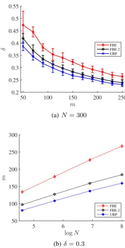
In this section, we present the results of experiments we conduct to validate our theory and compare the perfor-mance of the following three algorithms we discussed: uni-form random projection (URP) (Algorithm1), fast binary embedding (FBE) (Algorithm2) and the alternative fast bi-nary embedding (FBE-2) (Algorithm 3). We first apply these algorithms to synthetic datasets. In detail, given pa-rameters(N, p), a synthetic dataset is constructed by sam-plingNpoints fromSp−1uniformly at random. Recall that δis the maximum embedding distortion among all pairs of points. We use m to denote the number of binary mea-surements. Algorithm FBE needs parametersn, B, which are intermediate dimension and number of blocks respec-tively. Based on Theorem3.8,nis required to be propor-tional tom(up to some logarithmic factors) andB is re-quired to be proportional tologN. We thus setn≈1.3m, B ≈1.8 logN. We also setn ≈1.3mfor FBE-2. In ad-dition, we fixp= 512. We report our first result showing the functional relationship between(m, N, δ)in Figure1. In particular, panel1(a)shows the the change of distortion
Number of retrieved images 20 40 60 80 100 Recall 0.2 0.4 0.6 0.8 FBE FBE-2 FBE-2(same time) URP URP(same time) (a)m= 5000
Number of retrieved images 20 40 60 80 100 Recall 0.4 0.6 0.8 1 FBE FBE-2 FBE-2(same time) URP URP(same time) (b)m= 10000
Number of retrieved images 20 40 60 80 100 Recall 0.4 0.6 0.8 1 FBE FBE-2 FBE-2(same time) URP URP(same time) (c)m= 15000
Figure 2.Image retrieval results on Flickr-25600. Each panel presents the recall for specified number of measurementsm. Black and blue dot lines are respectively the recall of FBE-2 and URP with less number of measurements but the same running time as FBE.
δ over the number of measurementsm for fixedN. We observe that, for all the three algorithms,δdecays withm at the rate predicted by Proposition2.2and Theorem3.8. Panel1(b)shows the empirical relationship betweenmand logNfor fixedδ. As predicted by our theory (lower bound and upper bound),mhas a linear dependence onlogN. A popular application of binary embedding is image re-trieval, as considered in (Gong & Lazebnik,2011; Gong et al.,2013;Yu et al.,2014). We thus conduct an experi-ment on the Flickr-25600 dataset that consists of10k im-ages from Internet. Each image is represented by a 25600-dimensional normalized Fisher vector. We take500 ran-domly sampled images as query points and leave the rest as base for retrieval. Therelevant imagesof each query are defined as its10nearest neighbors based on geodesic dis-tance. Givenm, we apply FBE, FBE-2 and URP to convert all images intom-dimensional binary codes. In particular, we setB = 10for FBE andn≈1.3mfor FBE and FBE-2. Then we leverage the corresponding similarity metrics, (3.5) for FBE and Hamming distance for FBE-2 and URP, to retrieve the nearest images for each query. The perfor-mance of each algorithm is characterized byrecall, i.e., the number of retrieved relevant images divided by the total number of relevant images. We report our second result in Figure 2. Each panel shows the average recall of all queries for a specifiedm. We note that FBE-2, as a fast algorithm, performs as well as URP with the same num-ber of measurements. In order to show the running time advantage of our fast algorithm FBE, we also present the performance of FBE-2 and URP with fewer measurements such that they can be computed with the same time as FBE. As we observe, with large number of measurements, FBE-2 and URP perform marginally better than FBE while FBE has a significant improvement over the two algorithms un-der identical time constraint.
m 50 100 150 200 250 δ 0.2 0.25 0.3 0.35 0.4 0.45 0.5 0.55 FBE FBE-2 URP (a)N= 300 logN 5 6 7 8 m 50 100 150 200 250 300 FBE FBE-2 URP (b)δ= 0.3
Figure 1.Results on synthetic datasets. (a) Each point, along with the standard deviation represented by the error bar, is an average of50trials each of which is based on a fresh synthetic dataset with sizeN = 300and newly constructed embedding mapping. (b) Each point is computed by slicing atδ= 0.3in similar plots like (a) but with the correspondingN.
Acknowledgments
C. Caramanis and X. Yi were supported by NSF grants 1056028, 1302435 and 1116955. This research was also partially supported by the U.S. Department of Transporta-tion through the Data-Supported TransportaTransporta-tion OperaTransporta-tions and Planning (D-STOP) Tier 1 University Transportation Center.
References
Ailon, Nir and Chazelle, Bernard. Approximate nearest neighbors and the fast johnson-lindenstrauss transform. InProceedings of the thirty-eighth annual ACM sympo-sium on Theory of computing, pp. 557–563. ACM, 2006. Ailon, Nir and Liberty, Edo. An almost optimal un-restricted fast johnson-lindenstrauss transform. ACM Transactions on Algorithms (TALG), 9(3):21, 2013. Ailon, Nir and Rauhut, Holger. Fast and rip-optimal
trans-forms.Discrete & Computational Geometry, 52(4):780– 798, 2014.
Alon, Noga. Problems and results in extremal combina-toricsâ ˘AˇTi. Discrete Mathematics, 273(1):31–53, 2003. Andoni, Alexandr and Indyk, Piotr. Near-optimal hashing
algorithms for approximate nearest neighbor in high di-mensions. InFoundations of Computer Science, 2006. FOCS’06. 47th Annual IEEE Symposium on, pp. 459– 468. IEEE, 2006.
Cheraghchi, Mahdi, Guruswami, Venkatesan, and Vel-ingker, Ameya. Restricted isometry of fourier matrices and list decodability of random linear codes.SIAM Jour-nal on Computing, 42(5):1888–1914, 2013.
Gong, Yunchao and Lazebnik, Svetlana. Iterative quantiza-tion: A procrustean approach to learning binary codes. In Computer Vision and Pattern Recognition (CVPR), 2011 IEEE Conference on, pp. 817–824, 2011.
Gong, Yunchao, Kumar, Sanjiv, Rowley, Henry A, and Lazebnik, Svetlana. Learning binary codes for high-dimensional data using bilinear projections. InComputer Vision and Pattern Recognition (CVPR), 2013 IEEE Conference on, pp. 484–491. IEEE, 2013.
Jacques, Laurent, Laska, Jason N, Boufounos, Petros T, and Baraniuk, Richard G. Robust 1-bit compressive sensing via binary stable embeddings of sparse vectors. arXiv preprint arXiv:1104.3160, 2011.
Jayram, TS and Woodruff, David P. Optimal bounds for johnson-lindenstrauss transforms and streaming prob-lems with subconstant error. ACM Transactions on Al-gorithms (TALG), 9(3):26, 2013.
Johnson, William B and Lindenstrauss, Joram. Extensions of lipschitz mappings into a hilbert space.Contemporary mathematics, 26(189-206):1, 1984.
Krahmer, Felix and Ward, Rachel. New and improved johnson-lindenstrauss embeddings via the restricted isometry property.SIAM Journal on Mathematical Anal-ysis, 43(3):1269–1281, 2011.
Krahmer, Felix, Mendelson, Shahar, and Rauhut, Holger. Suprema of chaos processes and the restricted isometry property. Communications on Pure and Applied Mathe-matics, 67(11):1877–1904, 2014.
Ledoux, Michel and Talagrand, Michel. Probability in Ba-nach Spaces: isoperimetry and processes, volume 23. Springer, 1991.
Nelson, Jelani, Price, Eric, and Wootters, Mary. New con-structions of rip matrices with fast multiplication and fewer rows. In Proceedings of the Twenty-Fifth An-nual ACM-SIAM Symposium on Discrete Algorithms, pp. 1515–1528. SIAM, 2014.
Norouzi, Mohammad, Blei, David M, and Salakhutdinov, Ruslan. Hamming distance metric learning. InAdvances in Neural Information Processing Systems, pp. 1061– 1069, 2012.
Plan, Yaniv and Vershynin, Roman. Robust 1-bit com-pressed sensing and sparse logistic regression: A con-vex programming approach. Information Theory, IEEE Transactions on, 59(1):482–494, 2013.
Plan, Yaniv and Vershynin, Roman. Dimension reduction by random hyperplane tessellations.Discrete & Compu-tational Geometry, 51(2):438–461, 2014.
Raginsky, Maxim and Lazebnik, Svetlana. Locality-sensitive binary codes from shift-invariant kernels. In Advances in neural information processing systems, pp. 1509–1517, 2009.
Rudelson, Mark and Vershynin, Roman. On sparse recon-struction from fourier and gaussian measurements. Com-munications on Pure and Applied Mathematics, 61(8): 1025–1045, 2008.
Salakhutdinov, Ruslan and Hinton, Geoffrey. Semantic hashing. International Journal of Approximate Reason-ing, 50(7):969–978, 2009.
Weiss, Yair, Torralba, Antonio, and Fergus, Rob. Spectral hashing. InAdvances in neural information processing systems, pp. 1753–1760, 2009.
Yu, Felix X, Kumar, Sanjiv, Gong, Yunchao, and Chang, Shih-Fu. Circulant binary embedding. arXiv preprint arXiv:1405.3162, 2014.