Visualization of Program Dependence and Slices
Jens Krinke
FernUniversit¨at in Hagen, Germany
[email protected]
Abstract
The program dependence graph (PDG) itself and the computed slices within the program dependence graph are results that should be presented to the user in a comprehen-sible form, if not used in subsequent analyses. A graphical presentation would be preferred as it is usually more intu-itive than textual ones. This work describes how a layout for the PDGs can be generated to enable an appealing presen-tation. However, experience shows that the graphical pre-sentation is less helpful than expected and a textual presen-tation is superior. Therefore this work contains an approach to textually present slices of PDGs in source code. The in-novation of this approach is the fine-grained visualization of arbitrary node sets based on tokens and not on complete lines like in other approaches.
Furthermore, a major obstacle in visualization and com-prehension of slices is the loss of locality. Thus, this work presents a simple, yet effective, approach to limit the range of a slice. This approach enables a visualization of slices where the local effects stand out against the more global effects. A second, more sophisticated approach visualizes the influence range of chops for variables and procedures. This enables a visualization of the impact of procedures and variables on the complete system.
1. Introduction
A slice extracts those statements from a program that po-tentially have an influence on a specific statement of inter-est which is the slicing criterion. Slicing has found its way into various applications. Nowadays it is probably mostly used in the area of software maintenance and reengineer-ing [15], as in testreengineer-ing [17, 6, 5, 7], impact analysis [15] and cohesion measurement [24].
Originally, slicing was defined by Weiser in 1979; he presented an approach to compute slices based on itera-tive data flow analysis [31, 32]. The other main approach to slicing uses reachability analysis in program dependence graphs (PDGs) [11]. Program dependence graphs mainly
consist of nodes representing the statements of a program as well as control and data dependence edges:
• Control dependence between two statement nodes ex-ists if one statement controls the execution of the other (e.g. through if- or while-statements).
• Data dependence between two statement nodes exists if a definition of a variable at one statement might reach the usage of the same variable at another state-ment.
A slice can now simply be computed in three steps: Map the slicing criterion on a node, find all backward reachable nodes, and map the reached nodes back on the statements.
For the interprocedural variants IPDG and SDG the graphs are extended with additional interprocedural edges [18] (which are not discussed here). Our work is based on fine-grained dependence graphs, where the nodes are rep-resenting operands and operations (and thus a subset of the tokens) instead of statements.
The (backward) sliceS(n)of an IPDGG = (N, E)at noden∈N consists of all nodes on whichn(transitively) depends via an interprocedurally realizable path:
S(n) ={m∈N |m→? Rn}
Here,m →?
R ndenotes that there exists an
interprocedu-rally realizable path frommton. A forward slice consists of all nodes that (transitively) depend onn.
The program dependence graph itself and the computed slices within the program dependence graph are results that should be presented to the user if not used in subsequent analyses. As graphical presentations are often more intu-itive than textual ones, a graphical visualization of PDGs is desirable. The next section describes how a layout for the PDGs can be generated to enable an appealing presen-tation. The presented visualizations were used with differ-ent users. The project started together with a measuremdiffer-ent system certifying authority, where slicing was used to de-tect illegal influences on the measured values. The project members of the authority formed the first groups; they un-derstood the concepts of program dependence and slicing. The other group consisted of researchers and students doing
slicing research not necessarily related to the project. Both groups experience shows that the graphical presentation is less helpful than expected and a textual presentation is su-perior. Therefore Section 3 contains an approach to present slices in (fine-grained) PDGs textually in source code.
Furthermore, a major obstacle in visualization and com-prehension of slices is the loss of locality. Thus, Section 4 presents a simple, yet effective, approach to limit the range of a slice. A second, more sophisticated approach in Sec-tion 5 visualizes the influence range of chops for variables and procedures. A discussion of related work and conclu-sions follow.
2. Graphical Visualization of PDGs
Layout of graphs is a widely explored research field with many general solutions available in many graph drawing tools. Some of these tools have been tested to lay out PDGs. The primary goal was to provide an aid for the developers of the slicing system to debug and verify generated PDGs. The tools we tried have been:
daVinci a visualization system for generating high-quality
drawings of directed graphs [12].
VCG (Visualization of Compiler Graphs) is targeted at
the visualization of graphs that typically occur as data structures in programs [26].
dot is a widely-used tool to create hierarchical layouts of
directed graphs [21, 16].
The graphical representations generated by these tools have only been used by the slicing specialists, and their ex-perience has been disillusioning. The resulting layouts were visually appealing but unusable, as it was not possible to comprehend the graph. The reason is that the viewer has no cognitive mapping back to the source code, which is the rep-resentation he or she is used to. The user (the slicing special-ist) expects a representation that is either similar to the ab-stract syntax tree (as a presentation of the syntactical struc-ture), or a control-flow-graph like presentation.
In a second experiment the layout was influenced as much as possible to generate a presentation that enables the viewer to map the graph structure to the syntactical struc-ture based on the control-dependence subgraph. The con-trol dependence subgraph is tree-like, and in structured pro-grams it resembles the abstract syntax tree. The possibilities of influencing the layout were quite different in the evalu-ated tools, where dot had the greatest flexibility. However, it was not possible to manipulate the layout in a way that generated comprehensible presentations. The main obsta-cles have been:
1. The order of nodes was completely different than the order of the corresponding statements and their im-plicit control flow.
2. Nodes that were near in the laid out graph often had very distant statements in the source code.
3. It was hard to follow the data dependence edges. These obstacles made the general tools practically unusable for visualization of program dependence graphs.
2.1. A Declarative Approach to Lay out PDGs
As the general algorithmic approach to lay out PDGs had failed, a declarative approach has been implemented. The main goal of this approach is to eliminate the three obsta-cles mentioned before. It is based on the following observa-tions about the general properties of a PDG:
1. The control-dependence subgraph is similar to the structure of the abstract syntax tree.
2. Most edges in a PDG are data dependence edges. Usu-ally, a node with a variable definition has more than one outgoing data dependence edge.
The first observation leads to the requirement to have a tree-like layout of the control-dependence subgraph with the additional requirement that the order of the nodes in a hi-erarchy level should be the same as the order of equivalent statements in the source code. This is essential as the or-der of statements implies control flow, which is not explic-itly visualized in the layout (comprehension of the layout is much easier if the nodes’ statements are executed left-to-right). The second observation leads to an approach where the data dependence edges should be added to the result-ing layout without modifyresult-ing it. As most data dependence edges would now cross large parts of the graph, a Manhat-tan layout is adequate. This enables an orthogonal layout of edges with fixed start and end points.
2.1.1. Layout of the Control Dependence Graph
Instead of a specialized tree layout, an available implemen-tation of the Sugiyama algorithm [30] has been reused, con-sisting of three phases:
1. The nodes are arranged into a vertical hierarchy based on a spanning tree of the graph. Also, the number of levels crossed by edges is minimized.
2. Nodes in a horizontal level of the hierarchy are ordered to minimize the number of edge crossings.
3. The coordinates of the nodes are calculated such that long edges are as straight as possible.
Because the control dependence graph is mainly a tree, phase one is simple and very fast. Phase two has been replaced completely as the order of nodes is defined by the statement order in the source code and is not allowed to change. In Phase three the original algorithm has been extended with a “rubber-band” improvement presented in [26].
2.1.2. Layout of Data Dependence Edges
The layout of data dependence edges is basically a routing between fixed start and end points. As most edges in a PDG are data dependence edges, the routing must be fast and ef-ficient. Based on the observations at the beginning of this section, the routing is done according to the following prin-ciples:
1. The route of an edge is separated into three parts:
• a vertical segment between the start node and the level above the end node,
• a horizontal segment to the position of the end node, and
• a vertical end segment to the end node.
2. Edges leaving the same node share the same first seg-ment.
The layout of the three segments is done independently: The starting vertical segment is laid out straight if a node that would be crossed can be pushed aside. If this is not pos-sible, the segment is split to circumvent the node. The hor-izontal segment is laid out with a sweep-line algorithm to minimize the space routes take passing a level. The third segment is routed to its entry point into the end node.
2.1.3. Presentation of System Dependence Graphs
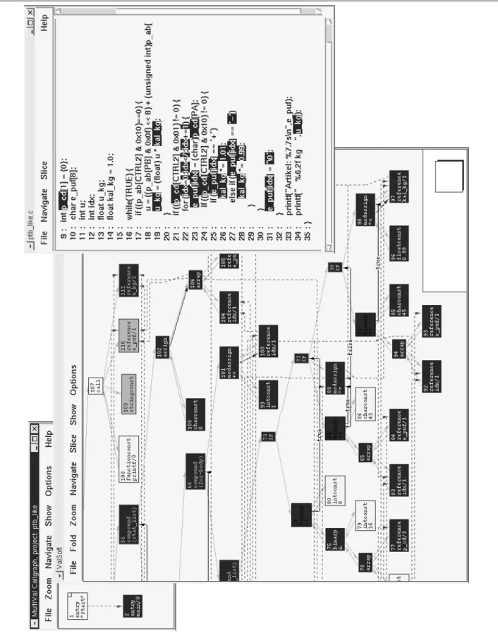
The presented approach to laying out PDGs has been imple-mented in a tool that visualizes system dependence graphs [9]. Starting from a graphical presentation of the call graph, the user can select procedures and visualize their PDGs. Through selection of nodes, slices can be calculated and are visualized through inverted nodes in the laid out PDGs. Pro-cedure crossing edges are visualized in the PDGs with an-chors, indicating that the edge leaves the current procedure. A visualization can be seen in Figure 1, where a slice is visualized in the dependence graph and source code through highlighting. Actually, the intersection of a forward and a backward slice is visualized there. The backward slice con-tains all statements that can influence the value of variable ‘u_kg’ in line 34, corresponding to node 111, and the for-ward slice contains all the statements that are influenced by variable ‘p_cd’ in line 9. The intersection1 shows all statements that are involved in an influence of ‘p_cd’ on ‘u_kg’.
2.1.4. Navigation
The user interface for the visualized graph contains exten-sive navigational aids:
• Nodes and edges can be searched for by their at-tributes.
1 Actually not the intersection is computed, but a chop [20], which is different to the intersection in the interprocedural case.
• Edges can be followed forward or backward.
• Selection of the anchors of a procedure crossing edge switches to the graph of the other procedure.
• A set of nodes can be expanded with all nodes reach-able by traversing one edge.
• The visualization can be focused on each node of a node set by stepping through the set.
• Node sets can be saved and restored.
• Two node sets can be combined to a new node set by set operations.
• Node sets can be “filtered” through external tools; slic-ing and choppslic-ing is implemented that way.
• To compress the visualized graph, node sets can be folded to a single node.
As discussed later, the user interface includes a textual vi-sualization of the source code. Most of the navigational aids are also present there.
2.2. Evaluation
The presented tool is used by all researchers and students involved in slicing research. Their experiences show that the layout is very comprehensible up to medium sized proce-dures and the user easily keeps a cognitive map from the structure of the graph to the source code and vice versa. This mapping is supported by the possibility of switching to a source code visualization of the current procedure and back: Sets of nodes marked in the graph can be highlighted in the source code and marked regions in the source code can be highlighted in the graph (see Figure 1 for an exam-ple). Together with the navigational aids, it is easy to see what statements influence which other statements and how. This is an important advancement to general purpose graph visualization tools, which are not able to provide the user with a comprehensible representation even for small proce-dures.
However, experience has shown that the graphical visu-alization is still too complex for large procedures. There, the number of nodes and edges is too big and it takes very long to follow edges across multiple pages by scrolling. Ad-ditionally, the users of the certifying authority were not able to use the graphical visualization. Although they understood the concepts of slicing and dependences, they were not able to use the tool to search for the reasons of a discovered il-legal influence (i.e. why a certain statement is in a slice). We therefore reverted to textual visualization, which is pre-sented next.
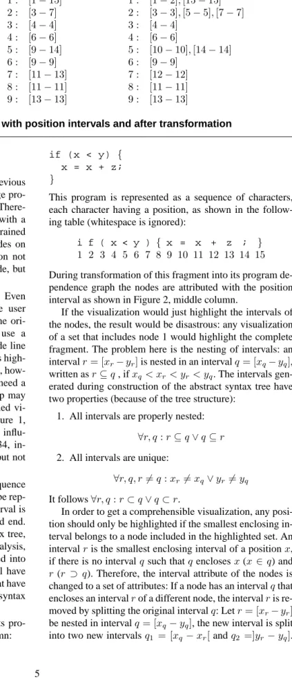
1 : [1−15] 2 : [3−7] 3 : [4−4] 4 : [6−6] 5 : [9−14] 6 : [9−9] 7 : [11−13] 8 : [11−11] 9 : [13−13] 1 : [1−2],[15−15] 2 : [3−3],[5−5],[7−7] 3 : [4−4] 4 : [6−6] 5 : [10−10],[14−14] 6 : [9−9] 7 : [12−12] 8 : [11−11] 9 : [13−13]
Figure 2. A small code fragment with position intervals and after transformation
3. Textual Visualization of Slices
The graphical visualization presented in the previous section has been found to be overly complex for large pro-grams and non-intuitive for visualization of slices. There-fore the graphical visualization has been extended with a visualization in source code. Because of the fine-grained structure, this causes a non-trivial projection of nodes on source code. The technique presented in this section not only visualizes slices (and chops [20]) in source code, but any set of nodes.
Textual visualization of source code is essential. Even with an accompanying graphical visualization, the user needs the reference to the source code to explain the ori-gins of dependences. Most current slicing tools use a line-by-line visualization: if any part of a source code line is included in the visualized slice, the complete line is high-lighted. This might be sufficient for traditional slicing, how-ever, more advanced techniques like chopping [20] need a more fine-grained visualization. For example, a chop may contain only parts of an expression and a fine-grained vi-sualization provides more precise information. Figure 1, line 19, contains such a situation: The detected influ-ence of variable ‘p_cd’, line 9, on ‘u_kg’, line 34, in-volves variables ‘u_kg’ and ‘kal_kg’ in line 19, but not variable ‘u’.
The source code is represented as a continuous sequence of characters, such that any piece of source code can be rep-resented as an interval in that sequence. Such an interval is described by a file/row/column position for start and end. During parsing while constructing the abstract syntax tree, every node is attributed with an interval. During analysis, the nodes of the abstract syntax tree are transformed into nodes in the program dependence graph, which still have the source code interval attribute (except for nodes that have no correspondence in the source code or the abstract syntax tree).
Consider the following example fragment with its pro-gram dependence graph shown in Figure 2, left column:
if (x < y) { x = x + z; }
This program is represented as a sequence of characters, each character having a position, as shown in the follow-ing table (whitespace is ignored):
i f ( x < y ) { x = x + z ; } 1 2 3 4 5 6 7 8 9 10 11 12 13 14 15
During transformation of this fragment into its program de-pendence graph the nodes are attributed with the position interval as shown in Figure 2, middle column.
If the visualization would just highlight the intervals of the nodes, the result would be disastrous: any visualization of a set that includes node 1 would highlight the complete fragment. The problem here is the nesting of intervals: an intervalr= [xr−yr]is nested in an intervalq= [xq−yq], written asr⊆q, ifxq < xr< yr< yq. The intervals gen-erated during construction of the abstract syntax tree have two properties (because of the tree structure):
1. All intervals are properly nested:
∀r, q:r⊆q∨q⊆r
2. All intervals are unique:
∀r, q, r6=q:xr6=xq∨yr6=yq It follows∀r, q:r⊂q∨q⊂r.
In order to get a comprehensible visualization, any posi-tion should only be highlighted if the smallest enclosing in-terval belongs to a node included in the highlighted set. An intervalris the smallest enclosing interval of a positionx, if there is no intervalqsuch thatqenclosesx(x∈q) and
r(r ⊃ q). Therefore, the interval attribute of the nodes is changed to a set of attributes: If a node has an intervalqthat encloses an intervalrof a different node, the intervalris re-moved by splitting the original intervalq: Letr= [xr−yr] be nested in intervalq= [xq−yq], the new interval is split into two new intervalsq1 = [xq −xr[andq2 =]yr−yq].
If this transformation is applied thoroughly, every interval will be unique.
The resulting intervals for the example are shown in Fig-ure 2, right column.
The nodes are now mapped to non-overlapping intervals. To highlight any set of nodes, the sets of intervals of the nodes are joined and only the intervals in the resulting set are highlighted.
The fragment below shows the visualization of a back-ward slice for node 9, which consists of the node set
{1,2,3,4,5,7,9}:
if (x < y) { x = x + z; }
The next example shows the node set{1,5,6}highlighted.
if (x < y) { x = x + z; }
We have presented only the basic visualization tech-niques. These techniques enable a fine-grained visualization of slices and arbitrary node sets in the source code. Most earlier approaches only visualize based on lines of source code, which is not sufficient for more advanced slicing tech-niques like chopping.
4. Distance-Limited Slices
Independent of visualization, one of the problems in un-derstanding a slice for a criterion is to decide why a spe-cific statement is included in that slice and how strong the influence of that statement is on the criterion. A slice can-not answer these questions as it does can-not contain any qual-itative information. Probably the most important attribute is locality: Users are more interested in facts that are near the current point of interest than on those far away. A sim-ple but very useful aid is to provide the user with naviga-tion along the dependences: For a selected statement, show all statements that are directly dependent (or vice versa). Such navigation is central to the VALSOFT system [23] or to CodeSurfer [1]. However, such navigational aids don’t offer an instant insight into the local effects of a statement.
A more general approach to accomplish locality in slic-ing is to limit the length of a path between the criterion and the reached statement. Using paths in program dependence graphs has an advantage over paths in control flow graphs: a statement having a direct influence on the criterion will be reached by a path with the length one, independent of the textual or control flow distance.
The distance-limited sliceS(c, k)of a PDG for the slic-ing criterion nodecconsists of all nodes on whichc (transi-tively) depends via a realizable path consisting of at mostk
0 20 40 60 80 100 0 10 20 30 40 50 60 70 80 90 100
percentage of the full slice
length limit k flex gnugo cdecl plot2fig agrep football simulator patch assembler bison lex315 ctags diff ansitape rolo compiler
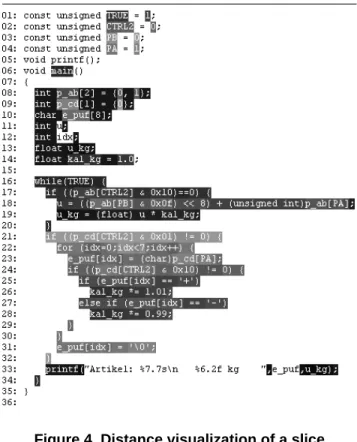
Figure 3. Evaluation of length-limited slicing
edges:
S(c, k) = {m| p=m→? Rc
∧p=hn1, . . . , nli ∧l < k} A nodemis said to have a distancel=d(m, n)from a node
n, if a realizable path frommtonconsisting ofledges ex-ists and no other path with fewer edges exex-ists:
d(m, n) =min({l|p=m→?
Rn∧p=hn1, . . . , nli}) An efficient distance-limited slicing algorithm is a mod-ified version of the interprocedural slicing algorithm [18, 22]. To omit a priority queue sorted by the actual distance, a breadth-first search is done where the worklist is implic-itly sorted.
Figure 3 shows an evaluation: For a series of test cases, the average size of 1000 length limited slices has been com-puted, where the length limit ranges from 1 to 100 (x-axis). The y-axis shows the reached percentage of the full slices. This evaluation shows that length limited slices be-have quite similar and independent of the analyzed pro-gram. Details of the test cases can be found in [22].
A more fine-grained approach is to replace the number of traversed edges by summarizing distances that have been assigned to the edges. Such distances can be used to give different classes of edges different weights. For example, a node that is reachable by a data dependence edge might be considered nearer than a node that is reachable by a sum-mary edge. If the worklist is replaced by a priority queue sorted by the current sum of distances, the previous algo-rithm is able to compute such distance-limited slices.
Distance-limited slices can be visualized with the tech-niques presented in the previous sections without any mod-ification. Another possibility is to illustrate the distances from the (slicing) criterion for any node in the (possibly
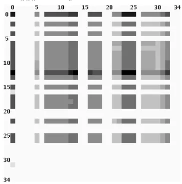
Figure 4. Distance visualization of a slice
distance-limited) slice. The textual visualization of Sec-tion 3 is therefore modified not only to highlight the nodes in the textual representation, but to give any source code fragment a color representing the distance of the equivalent nodes to the criterion. The slicing algorithm does not need to be changed to accommodate the distance computation— it is sufficient to remember the distance of a node during breadth-first search.
Figure 4 shows an example visualization of a slice. A backward slice for variable ‘u_kg’ in line 33 is displayed. Parts of the program that have a small distance to the slic-ing criterion are darker than those with a larger distance. With this presentation one can see that the initialization in lines 8–10 and 13–14 have a close influence on the crite-rion. It can also be seen that the first few lines of the loop (17–19) have a close influence and that the whole next if-statement has a varying influence, where lines 26 and 28 have the strongest effect. This visualization immediately shows why there is an influence of the variable ‘kal_kg’ in lines 26 and 28 on ‘u_kg’ in the criterion: The statement 19 uses ‘kal_kg’ to compute a new value for ‘u_kg’. De-spite the fact that statement 19 is textually far away from the criterion, the dark color shows its strong influence. Such in-formation would not be visible in a simple slice visualiza-tion (e.g. Figure 1); the visualizavisualiza-tion of the distance guides the viewer to the important areas in the slice.
5. Abstract Visualization
For program understanding in-the-small the presented visualization techniques are very effective. However, for program understanding in-the-large they are not as helpful. If an unknown program is analyzed, the very detailed infor-mation of program dependence and slices is overwhelming and a much less detailed information is needed. The user trying to understand the program will start with variables and procedures and not with statements. To understand a previously unknown program, it is helpful to identify the ‘hot’ procedures and global variables—the procedures and variables with the highest impact on the system.
This section shows how slicing and chopping can help to visualize programs in a more abstract way, illustrating relations between variables or procedures. Chopping [20] reveals the statements involved in a transitive dependence from one specific statement (the source criterion) to another (the target criterion). A chop for a chopping criterion(s, t)
is the set of nodes that are part of an influence of the (source) nodeson the (target) nodet: The chopC(s, t)of an IPDG
G = (N, E)from the source criterion s ∈ N to the tar-get criteriont ∈ N consists of all nodes on which node
t(transitively) depends via an interprocedurally realizable path from nodesto nodet:
C(s, t) ={n∈N | p∈s→? Rt
∧p=hn1, . . . , nli
∧ ∃i:n=ni}
5.1. Variables or Procedures as Criterion
It is possible to define slices for variables or procedures as criteria informally:
1. A (backward) slice for a criterion variablevis the set of statements (or nodes in the PDG) which may influ-ence variablevat some point of the program.
2. A (backward) slice for a criterion procedureP is the set of statements (or nodes in the PDG) which may in-fluence a statement ofP.
These definitions can be adapted to the other slicing and chopping variants, including the adaptation of the needed algorithms. It will not be presented here, as it is straightfor-ward.
5.2. Visualization of the Influence Range
As previously noted, it is helpful to identify the ‘hot’ pro-cedures and global variables. However, to identify them, we have to measure the procedures’ and variables’ impact on the system. A simple measurement is to compute slices for every procedure or global variable and record the size of the computed slices. However, this might be too simple and
a slightly better approach is to compute chops between the procedures or variables. A visualization tool has been im-plemented that computes an×nmatrix fornprocedures or variables, where every elementni,j of the matrix is the size of a chop from the procedure or variablenj toni. The matrix is painted using a color for every entry, correspond-ing to the size—the bigger, the darker. Figure 5 shows such a visualization for theansitapeprogram. The columns show variables 0–34 as source criteria and the rows as tar-get criteria. This matrix can be interpreted as follows:
• The global variables ‘stdin’ (column two), ‘stdout’ (3) and ‘stderr’ (4) have empty chops with all other variables (light columns 2–4). This is ob-vious for ‘stdout’ and ‘stderr’ while ‘stdin’ has no influence because the program only reads from tapes.
• The variable ‘stdout’ (row 3) is not influenced (empty chops with stdout as target criterion), but ‘stderr’ (row 4) is. The ansitape program nor-mally writes all messages to ‘stderr’ and produces no other output (except for writing to tapes).
• Row 12 has the biggest chops (and is the darkest row). This is variable ‘tcb’, the tape control block, which is the main global variable of the program.
An implementation is shown in Figure 6: The three win-dows contain the chop matrix visualization (in this case for procedure-procedure-chops), a color scale and a window that shows the names of the procedures and their chop’s size for the last chosen matrix element. With this tool, it is easy to get an overall impression of the software to ana-lyze. Important procedures or global variables can be iden-tified at first sight and their relationship be studied. Doing this as a preparing stage aids in later, more thorough inves-tigations with traditional slicing visualizations like the ones presented in the previous sections.
6. Related Work
The SeeSlice slicing tool [3] includes some of the pre-sented focusing and visualization techniques (the distance-limited slicing and visualizing distances). Files and proce-dures are not presented through source code but with an ab-straction representing characters as single pixels. Files and procedures that are not part of computed slices are folded, such that only a small box is left. Slices highlight the pix-els corresponding to contained elements.
In [4] the same problems with visualizing dependence graphs are reported and a decomposition approach is pre-sented: Groups of nodes are collapsed into one node. The result is a hierarchy of groups, where every group is visual-ized independently. Three different decompositions are pre-sented: The first decomposition is to group the nodes
be-stdin stdout stderr tcb
Figure 5. Visualization of chops for all global variables
longing to the same procedure, the second is to group the nodes belonging to the same loop and the third is a combi-nation of both. The result of the function decomposition is identical to the visualization of the call graph and the PDGs of the procedures presented in Section 2.1.3.
The CANTO environment [2] has a visualization tool PROVIS based on dot which can visualize PDGs (among other graphs). Again, problems with exces-sively large graphs are reported, which are omitted by only visualizing the subgraph which is reachable from a cho-sen node via a limited number of edges. It can be used in a stepping mode which is similar to distance-limited slic-ing: At each step the slice grows by considering one step of data or control dependence.
ChopShop [20, 19] is a tool to visualize slices and chops, based on highlighting text (in emacs) or laying out graphs (with dot and ghostview). It is reported that even the small-est chops result in huge graphs. Therefore, only an ab-straction is visualized: normal statements (assignments) are omitted, procedure calls of the same procedure are folded into a single node and connecting edges are attributed with data dependence information.
The decomposition slice visualization of Surgeon’s As-sistant [14, 13] visualizes the inclusion hierarchy of decom-position slices as a graph using VCG [26].
An early system with capabilities for graphical visualiza-tion of dependence graphs is ProDAG [25]. Another system to visualize slices is [8].
Every slicing tool visualizes its results directly in the source code. However, most tools are line based, highlight-ing only complete lines. CodeSurfer [1] has textual visual-ization with highlighting parts of lines if there is more than one statement in a line. The textual visualization includes graphical elements like pop-ups for visualization and navi-gation along e.g. data and control dependence or calls. Such aids are necessary as a user cannot identify relevant depen-dences easily from source text alone. Such problems have also been identified by Ernst [10] and he suggested simi-lar graphical aids. However, his tool, which is not restricted to highlighting complete lines, does not have such aids and offers depth-limited slicing instead (see Section 4).
Steindl’s slicer for Oberon [27, 28, 29] also highlights only parts of lines, based on the individual lexical elements of the program.
CodeSurfer [1] also has a project viewer, which features a tree-like structural visualization of the SDG. This is use-ful for seeing “hidden” nodes, such as nodes that do not cor-respond to any source text.
7. Conclusions
All previous approaches to visualize slices and program dependence graphs in graph layouts used general purpose
graph visualization tools. None of them were able to gener-ate comprehensible visualizations of even small procedures. Our approach is the first with a dedicated, declarative ap-proach to lay out dependence graphs that generates com-prehensible graphs of small to medium sized procedures.
Despite the widespread use of graphical visualization in software maintenance and reverse engineering, our and oth-ers’ experiences for graphical visualization of program de-pendence and program slices are different. For tasks related to “understanding in-the-large” graphical visualization has proven to be successful. The main reason is that the number of nodes (or objects) to be visualized is kept very low by clustering techniques. Tasks related to “understanding in-the-small” like program dependence and program slices suf-fer from the sheer amount of data to be visualized. Even our approach for graphical visualization has problems for large procedures. Our and others’ experiences show that graphi-cal visualization has more disadvantages than advantages in this area. Users outside slicing research just don’t want to see the dependence graphs.
The visualization of slices in textual form has shown to be much more effective, because the programmer is accus-tomed to representations similar to source code. However, slices are still hard to understand, because the loss of lo-cality. Distance-limited slicing and its visualization helps, because it limits the distance of the influence to the current point of interest. The visualization of the distance shows im-mediately how important a statement is for the current in-fluence.
For program “understanding in-the-large” none of the detailed visualizations of slices are helpful. The presented approach to visualize the influence range of variables and procedures by visualizing the size of chops can help the user to identify “hot spots” of the program very fast. It success-fully generates a high-level abstraction of the procedures’ and variables’ impact on the complete system.
Acknowledgments. Much of the presented work has been done at Universit¨at Passau, Germany. Frank Ehrich imple-mented the graphical user interface and the graph lay out-ing. Daniel Gmach implemented the textual visualization. Silvia Breu implemented the chop visualization tool.
References
[1] P. Anderson and T. Teitelbaum. Software inspection using codesurfer. In Workshop on Inspection in Software Engi-neering (CAV 2001), 2001.
[2] G. Antoniol, R. Fiutem, G. Lutteri, P. Tonella, S. Zanfei, and E. Merlo. Program understanding and maintenance with the CANTO environment. In International Conference on Soft-ware Maintenance, pages 72–81, 1997.
[3] T. Ball and S. G. Eick. Visualizing program slices. In IEEE Symposium on Visual Languages, pages 288–295, 1994.
[4] F. Balmas. Displaying dependence graphs: a hierarchical ap-proach. In Proc. Eigth Working Conference on Reverse En-gineering, pages 261–270, 2001.
[5] S. Bates and S. Horwitz. Incremental program testing us-ing program dependence graphs. In Conference Record of the Twentieth ACM SIGPLAN-SIGACT Symposium on Prin-ciples of Programming Languages, pages 384–396, 1993. [6] D. Binkley. Using semantic differencing to reduce the cost of
regression testing. In Proceedings of the International Con-ference on Software Maintenance, pages 41–50, 1992. [7] D. Binkley. The application of program slicing to
regres-sion testing. Information and Software Technology, 40(11– 12):583–594, 1998.
[8] Y. Deng, S. Kothari, and Y. Namara. Program slice browser. In Ninth International Workshop on Program Comprehen-sion (IWPC’01), pages 50–59, 2001.
[9] F. Ehrich. Entwurf und Implementierung eines Werkzeugs zur Visualisierung von Programmabh¨angigkeitsgraphen. Diplomarbeit, TU Braunschweig, 1996. (In German). [10] M. D. Ernst. Practical fine-grained static slicing of
opti-mized code. Technical Report MSR-TR-94-14, Microsoft Research, Redmond, WA, July 1994.
[11] J. Ferrante, K. J. Ottenstein, and J. D. Warren. The program dependence graph and its use in optimization. ACM Trans. Prog. Lang. Syst., 9(3):319–349, July 1987.
[12] M. Fr¨ohlich and M. Werner. Demonstration of the interac-tive graph visualization system davinci. In R. Tamassia and I. G. Tollis, editors, Graph Drawing, DIMACS International Workshop GD’94, volume 894 of LNCS. Springer, 1995. [13] K. Gallagher and L. O’Brien. Reducing visualization
com-plexity using decomposition slices. In Software Visualization Workshop, pages 113–118, 1997.
[14] K. B. Gallagher. Visual impact analysis. In Proceedings of the International Conference on Software Maintenance, pages 52–58, 1996.
[15] K. B. Gallagher and J. R. Lyle. Using program slicing in software maintenance. IEEE Transactions on Software En-gineering, 17(8):751–761, 1991.
[16] E. R. Gansner, S. C. North, and K. P. Vo. DAG - A program that draws directed graphs. Software, Practice and Experi-ence, 18(11):1047–1062, 1988.
[17] R. Gupta, M. J. Harrold, and M. L. Soffa. An approach to regression testing using slicing. In Proceedings of the IEEE Conference on Software Maintenance, pages 299–308, 1992. [18] S. B. Horwitz, T. W. Reps, and D. Binkley. Interprocedural slicing using dependence graphs. ACM Trans. Prog. Lang. Syst., 12(1):26–60, Jan. 1990.
[19] D. Jackson and E. J. Rollins. Abstraction mechanisms for pictorial slicing. In Proceedings of the IEEE Workshop on Program Comprehension, pages 82–88, 1994.
[20] D. Jackson and E. J. Rollins. A new model of program de-pendences for reverse engineering. In Proceedings of the second ACM SIGSOFT Symposium on Foundations of Soft-ware Engineering, pages 2–10, 1994.
[21] E. Koutsofios and S. C. North. Drawing graphs with dot. Murray Hill, NJ, 1996.
[22] J. Krinke. Evaluating context-sensitive slicing and chopping. In International Conference on Software Maintenance, pages 22–31, 2002.
[23] J. Krinke and G. Snelting. Validation of measurement soft-ware as an application of slicing and constraint solving. Information and Software Technology, 40(11-12):661–675, Dec. 1998.
[24] L. M. Ott and J. M. Bieman. Program slices as an abstrac-tion for cohesion measurement. Informaabstrac-tion and Software Technology, 40(11-12):691–700, 1998.
[25] D. J. Richardson, T. O. O’Malley, C. T. Moore, and S. L. Aha. Developing and integrating prodag into the arcadia en-vironment. In Proceedings of the Fifth Symposium on Soft-ware Development Environments, pages 109–119, 1992. [26] G. Sander. Graph layout through the VCG tool. In R.
Tamas-sia and I. G. Tollis, editors, Proc. DIMACS Int. Work. Graph Drawing, GD’94, number 894 in LNCS, pages 194–205. Springer, 1995.
[27] C. Steindl. Intermodular slicing of object-oriented programs. In International Conference on Compiler Construction, vol-ume 1383 of LNCS, pages 264–278. Springer, 1998. [28] C. Steindl. Benefits of a data flow-aware programming
en-vironment. In Workshop on Program Analysis for Software Tools and Engineering (PASTE’99), 1999.
[29] C. Steindl. Program Slicing for Object-Oriented Program-ming Languages. PhD thesis, Johannes Kepler University Linz, 1999.
[30] K. Sugiyama, S. Tagawa, and M. Toda. Methods for visual understanding of hierarchical system structures. IEEE Trans-actions on Systems, Man, and Cybernetics, SMC-11(2):109– 125, Feb. 1981.
[31] M. Weiser. Program slices: formal, psychological, and practical investigations of an automatic program abstrac-tion method. PhD thesis, University of Michigan, Ann Ar-bor, 1979.
[32] M. Weiser. Program slicing. IEEE Trans. Softw. Eng., 10(4):352–357, July 1984.