A methodology for integrated risk management and
proactive scheduling of construction projects
Damien Schatteman, Willy Herroelen, Stijn Van de Vonder and Anton Boone
DEPARTMENT OF DECISION SCIENCES AND INFORMATION MANAGEMENT (KBI)
Faculty of Economics and Applied Economics
A methodology for integrated risk management
and proactive scheduling of construction projects
Damien Schatteman
∗∗Willy Herroelen
∗∗Stijn Van de Vonder
∗∗and Anton Boone
∗ ∗Belgian Building Research Institute (BBRI)
∗∗
Department of Decision Sciences and Information Management
Research Center for Operations Management
Faculty of Economics and Applied Economics
Katholieke Universiteit Leuven (Belgium)
Abstract
An integrated methodology is developed for planning construction projects under uncertainty. The methodology relies on a computer sup-ported risk management system that allows to identify, analyze and quan-tify the major risk factors and derive the probability of their occur-rence and their impact on the duration of the project activities. Us-ing project management estimates of the marginal cost of activity start-ing time disruptions, a proactive baseline schedule is developed that is sufficiently protected against the anticipated disruptions with acceptable project makespan performance. The methodology is illustrated on a real life application.
1
Introduction
Construction projects have to be performed in complex dynamic environments that are often characterized by uncertainty and risk. The literature contains ample evidence that many construction projects fail to achieve their time, bud-get and quality goals (Al-Bahar and Crandall (1990), Assaf and Al-Hejji (2006), Mulholland and Christian (1999)). Ineffective planning and scheduling has been recognized as a major cause of project delay (Assaf and Al-Hejji (2006), Mulhol-land and Christian (1999)). A study by Maes et al. (2006) revealed that inferior planning was the third major cause of company bankruptcies in the Belgian construction industry.
The objective of this paper is to describe a methodology for integrated risk management and proactive/reactive construction project scheduling. Risk man-agement in the construction industry has mostly been used for measuring the
im-pact of potential risks on global project parameters such as time and costs. The literature provides both fuzzy approaches and mixed quantitative/qualitative assessment and risk response methods (Mulholland and Christian (1999), Ben-David and Raz (2001), Carr and Tah (2001), Jannadi and Almishari (2003), Choi et al. (2004), Warszawski and Sacks (2004)). Many of the proposed methods, however, suffer from practical implementation failures because project teams generally are too preoccupied with solving current problems involved with get-ting work done and therefore have insufficient time to think about, much less carry out, a formal risk assessment program (Oglesby et al. (1989)). Unlike these approaches, we rely on an integrated methodology that not only allows for un-certainty estimation at the level of the individual project activities, but also uses this input for a proactive scheduling system to generate a robust baseline schedule that is sufficiently protected against anticipated disruptions that may occur during project execution while still guaranteeing a satisfactory project makespan performance.
The methodology relies on a computer supported risk management system that uses a graphical user interface to support project management in the iden-tification, analysis and quantification of the major project risk factors and to derive the probability of their occurrence as well as their impact on the dura-tion of the project activities. Using estimates on the marginal cost of activity starting time disruptions provided by project management, a buffer insertion algorithm is used to generate a proactive baseline schedule that is sufficiently protected against anticipated disruptions that may occur during project execu-tion without compromising on due date performance.
The organisation of this paper is as follows. In the next section we describe the computer supported risk management framework and proactive schedule generation system. We illustrate the working principles of the methodology on a real-life project in Section 3. The last section provides overall conclusions.
2
Integrated risk management framework
The literature provides a number of risk assessment procedures, but few of them manage to produce quantitative data (Lyons and Skitmore (2004)). Al-Bahar and Crandall (1990) propose a systematic risk assessment method in which the need for a quantitative risk assessment procedure is advocated.
In this paper, we introduce an integrated computer based risk management approach, that allows for the effective identification, analysis and quantification of the major risk factors and relies on a user friendly graphical user interface that prompts the project management team to provide the necessary data which allow to estimate the impact of the risk factors at the level of the individual project activities.
The system maintains a risk management database that is updated with new risk information generated by the project management teams of on-going projects and as such can serve as input for a proactive scheduling system. The system allows for the computation of the probability of occurrence of the risk
factors shared by groups of activities and allows for the estimation of their impact on the duration of the individual project activities. Using project man-agement estimates of the marginal cost of activity starting time disruptions, a robust scheduling system is used to derive proactive baseline schedules that are sufficiently protected against the anticipated disruptions without compromising the project makespan performance. The methodology is illustrated on a real life application.
The integrated system has been developed as the major project result of a joint project executed by the Belgian Building Research Institute (BBRI) and theResearch Center for Operations Management of K.U.Leuven (Belgium) under a grant offered by theInstitute for the Promotion of Innovation by Science and Technology in Flanders (IWT). It has been field tested at a number of real life project sites and has been fine tuned in cooperation with the project management teams of a number of construction companies operating in different sectors of the Belgian construction industry.
2.1
The risk management framework
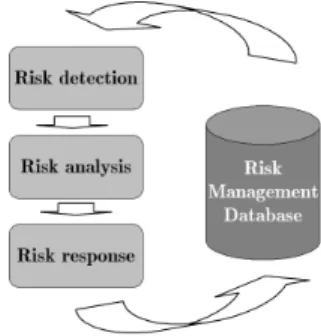
We follow the widely accepted view that risk management is an iterative process (see e.g. Al-Bahar and Crandall (1990), Chapman and Ward (2000) and PMI (2000)), involving risk identification, risk analysis and evaluation, risk response management, and the system administration supported by a risk management database (Figure 1).
2.1.1 Risk identification
During the project initiation phase, project management must decide on the major performance objectives (Demeulemeester and Herroelen (2002)). The objectives of a project refer to the end state that project management is trying to achieve and which can be used to monitor progress and to identify when a project is successfully completed. Among the traditional objectives of time, cost and quality, this paper will mainly focus on the delivery of the project result within a satisfactory project makespan (due date performance) relying on a stable project baseline schedule that helps to reduce the nervousness within the project supply chain.
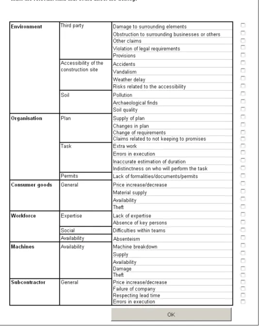
The risk identification process involves the identification of the major poten-tial sources of risk associated with the project objectives. Based on checklists of potential risks available in the literature and maintained at the Belgian Build-ing Research Institute (BBRI), a limited, workablelist of risk factor classes has been established (Figure 2). This list allows for the generation of sector and specialisation specific risk profiles of the construction industry.
Based on existing tender lists, project activities are grouped into a limited number ofactivity groups, containing activities with similar risk structure. Such activity grouping should not be confused with the aggregation of activities into work packages. In a work breakdown structure, the activities ’Painting the bedroom ceiling’ and ’Tiling the bedroom’, for example, can be aggregated into the activity ’Bedroom finalization’, while we are interested in grouping all painting activities that may suffer from similar potential risks together in a single activity group, regardless of where and when the individual group activities are executed.
Grouping the activities that share common risks into activity groups, sim-plifies the subsequent risk analysis process, which can now be performed at the activity group level rather than at the level of each individual project activity.
The identification of the relevant risk factors for an individual project relies on both the input of the project management team and an historicalrisk man-agement database that is maintained and continuously updated at the BBRI. This database can be consulted by the project management teams and as such serves as a continuously updated source of information for the risk identification and risk analysis process.
2.1.2 Risk analysis
Risk analysis involves the qualitative and quantitative assessment of the identi-fied risk factors. Project management has to estimate the probability of occur-rence of the risk factors as well as their potential impact. The risk management database can then be updated with the new information.
It is not possible to anticipate for all potential risks. Some risks may have such a rare occurrence and/or such big impact on the project that they can be classified as unpredictable special events. It is crucial, however, that the major predictable risk factors are effectively analysed and quantified. Some of the possible risk impacts may be an activity duration increase (in time units), a productivity decrease (in percentage of the required time) caused for example by bad weather conditions, a delay in the planned starting time of an activity, an increase in the cost of an activity, an increase in the required amount of renewable resources, etc.
Because resources are often shared among different projects, disruptions in one project can cause delays in other projects. Also the subcontractors may generate delays. When appointments with subcontractors cannot be met be-cause of delays in predecessor tasks, it may be difficult to fix new appointments at short notice. Ineffective planning and scheduling is an important delay cause (Assaf and Al-Hejji (2006)).
Estimating the project activity data For each activity in the various ac-tivity groups, project management has to estimate the time, resource and cost data that will be used in the baseline schedule generation process.
In no way, time contingency should be included in the individual activity duration estimates. On the contrary, activity durations must be derived using aggressive time estimates d∗j, without including any safety whatsoever. This means that we advocate the aggressive activity duration estimate to be based on the (unrealistic) best case activity duration, rather than on the mean or median duration as suggested by the critical chain approach of Goldratt (1997). For each activity group, the project manager must also specify theactivity weightwj to be assigned to each activity in the group. This weight represents a
marginal disruption cost of starting the activity during project execution earlier or later than planned in the baseline schedule. The weights reflect the scheduling flexibility of the activities in the groups and will be used by the robust project scheduling procedures described in Section 2.2.
A small activity weight reflects high scheduling flexibility or low instability cost: it does not ’cost’ that much if the actually realized activity starting time during schedule execution differs from the planned starting time in the base-line schedule. Activities that depend on resources with ample availability, for example, will be given a small weight. Their rescheduling cost is small.
A heavy weight reflects small scheduling flexibility: deviations between ac-tual and planned starting times are deemed very costly for the organisation (e.g. high penalties that are incurred when individual milestones or the project due date are not met). Activities that use scarce resources or use subcontractors that
are in a strong bargaining position will receive a heavy weight, since it is prefer-able that the starting time of these activities (or corresponding milestones) will be kept fixed in time as much as possible. Rescheduling these activities would create additional delays or cost increases.
The GUI shows a slider bar to capture the activity weight input. The slider bar shown in Figure 3 shows that the activity group ’Concrete pouring and polishing’ is considered as rather flexible. The reason for this can be that the activity is to be performed by the company’s own work force that is currently operating with flexible overcapacity. The GUI software translates the slider bar value into a numerical activity weightwj.
Figure 3: Interface to specify the flexibility of an activity
Constructing the project network The project scheduling procedure de-scribed in Section 2.2 assumes that the project is represented by an activity-on-the-node networkG(N, A), in which the node setNdenotes the set of activities, andAspecifies the precedence relations.
Our experience indicates that project managers tend to generate precedence relations that already reflect implicit scheduling decisions, rather than pure technologically based precedence constraints. For example, two activitiesaand b may be assigned a finish-start, zero-lag precedence relation by project man-agement, not because technological conditions impose such a relationship, but because both activities require the same resource that is available in a single unit, or because company tradition calls for executing activitya first. The re-sult is that a precedence and resource feasible schedule is generated for a project that will suffer from unnecessary precedence constraints, with an unjustified re-duction in scheduling flexibility, and an unnecessary propagation of scheduling conflicts caused by scheduling disruptions that may occur during project exe-cution.
Generating risk profiles The risk quantification procedure should be work-able for the project management team. Our approach is somewhat similar to the minimalist first pass approach of Chapman and Ward (2000). Similar to theirs, our approach expects project management to provide the probability of occurrence and the impact of the risk factors on the activities of an activity group under a best case scenario and a worst case scenario.
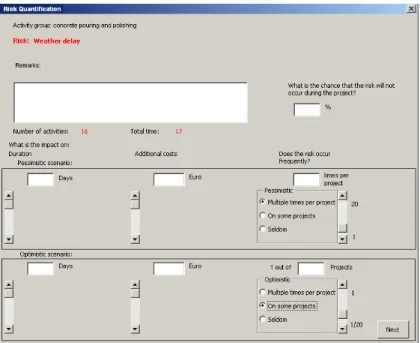
The graphical user interface (GUI) prompts the project manager to answer a list of scenario based questions. A print screen of an example question/answer session is shown in Figure 4. Upon validation, the answers provided by the project managers are directly entered in the GUI.
Figure 4: A graphical user interface for risk quantification
The following series of questions (Q) and answers (A) may constitute the input for the quantification of a risk and its impact on the duration increase of the activities of a certain activity group:
Q (1): Imagine a worst case scenario. How long will the affected activity duration be extended by this risk in the worst case scenario?
A (2): bdays
Q (3): Based on your past experience, what is the frequency that such a worst case scenario has appeared in a similar previous project?
A (4): ζ(b)
Q (5): Assume now that the risk occurs, but the prolongation of the affected activity duration can be limited as much as possible. What will this best case prolongation be?
Q (7): Based on your past experience, what is the frequency that such a best case scenario has appeared in a similar project?
A (8): ζ(a)
Q (9): Finally, what is the overall frequency that such a risk has appeared in similar projects?
A (10): q
The frequenciesζ(a), ζ(b) andqcan be larger than one if the project manager expects several occurrences of the risk during the project. The data are entered in the GUI after validation. A simple validation test states thatq≥ζ(a) +ζ(b). Otherwise, revision of the data by the project manager is required.
From the two extreme case point estimates, (aandb) a triangular probability density function f(x) and its cumulative distribution function F(x) for the impact x are generated. A triangular distribution is completely defined by three parameters, being the lower limit, the mode and the upper limit.
The first step to generate f(x) is the determination of c, the most likely estimate for the impact. Asking the project manager for an estimate ofc has been shown to be difficult because of the fuzziness inherent to the ”most likely” concept. Our approach proposes to calculatecinstead. For the time being, we assume that the best case scenarioaand the worst case scenariobare the lower and upper limit off(x) respectively. We find that
c= aζ(a) +bζ(b)
ζ(a) +ζ(b) (1) The reasoning behind this formula starts from the idea that project man-agers never think in terms of point estimatesf(x) for a continuous distribution. We do, however, assume that the fraction ζ(a)/ζ(b) is a correct estimate of P(a)/P(b) in which P(a) and P(b) (see Eq. (2) and (3)) must be interpreted as being the discrete probabilities that if the risk occurs, its impact lies within a certain scenario interval with width. reflects to what extent the project manager thinks in terms of scenarios and is highly dependent on the individual. ζ(a)/ζ(b) is thus regarded as the ratio that the best case scenario is thought to be more likely to occur than the worst case scenario.
P(a) = Z x=a+ x=a f(x)dx=F(a+) (2) P(b) = Z x=b x=b− f(x)dx= 1−F(b−) (3)
From Eq. (2) and Eq. (3) we may conclude that ζ(a) ζ(b) = P(a) P(b) = F(a+) 1−F(b−) (4) Next, the distribution function F(x) of a triangular distribution is known
and defined by:
F(x) =
( (x−a)2
(b−a)(c−a) fora≤x≤c
1−(b−(ba−)(xb)−2c) forc < x≤b (5)
Substituting Eq. (5) in Eq. (4) gives
ζ(a) ζ(b) = 2 (b−a)(c−a) 2 (b−a)(b−c) = b−c c−a (6)
Becauseb−c= (b−a)−(c−a),we find that
c=a+ b−a
1 + ζζ((ab)) (7)
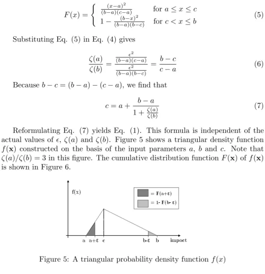
Reformulating Eq. (7) yields Eq. (1). This formula is independent of the actual values of, ζ(a) and ζ(b). Figure 5 shows a triangular density function f(x) constructed on the basis of the input parameters a, b and c. Note that ζ(a)/ζ(b) = 3 in this figure. The cumulative distribution functionF(x) off(x) is shown in Figure 6.
Figure 5: A triangular probability density functionf(x)
Deriving individual activity risk profiles The probability density func-tionsf(x) of the impacts for all detected risks, derived in the previous section at the level of the activity groups, have to be projected on the individual project activities. This projection is the key to the reusability of the risk assessments at the level of the activity groups. Using the characteristics of the risk impact densities and probability, risk assessments and/or risk data coming from project records, distributions for project activities can be calculated and entered in the risk management database.
In the previous section we described how the GUI was used to prompt the project manager to specify the average occurrence rateqof any risk in activity groupAG. To obtain the probability density functionf(x), we rather need the occurrence rate of the risk at the level of a single project activityj.
We assume that the number (k) of risk occurrences is Poisson distributed (see Eq. (8)) and that the rateλj at which the risk occurs for activityj can be
calculated by Eq. (9). f(k;λj) = e−λjλk j k! (8) λj = vj X ∀i∈AG vi q (9)
The weightsvidepend on the characteristics of the risk. If the risk occurrence
rate is independent ofdi(e.g. a license delay), we setvi=ui,whereuiis a binary
variable that equals 1 if the risk affects activityiand equals 0 otherwise. When the risk occurrence depends ondi, we setvi =di∗×ui,whered∗i is the aggressive
duration estimate of activityi.
Simulation can then be used to obtain a probability density functionf(dj)
for the activity durationdj. We start by simulating the number of occurrences
k which follows the distribution of Eq. (8). Then, for each occurrence l(l = 1, . . . , k), the inverse distribution functionx=F−1(y) can be used to generate
random valuesxlfor the risk impact, withydrawn from a uniform distribution
between 0 and 1.
Subsequently, the simulated activity durationdjis calculated as a function of
the aggressive activity durationd∗j and the simulated impactsxlfor eachl. How
this is done depends on the characteristics of the risk impact. For example, for risk factors that may lead to an activity duration increase - our major concern in this paper - we obtain the expected activity duration as:
dj =d∗j+ k
X
l=1
xl (10)
A sufficient number of simulation runs allow the generation of the distri-bution functionsf(dj).These simulated distribution functions are then fit into
known distribution functionsf∗. A triangular distribution, for example, is
aj enbj are directly distilled from the simulatedf andcj is calculated as
cj = 3×E(dj)−aj−bj (11)
Visibility for project managers is the main advantage of this approach. aj,
bj andcj refer to an optimistic, a pessimistic and a most likely estimate ofdj.
Validating the estimates The estimatesaj,bj andcj are the result of
sub-jective parameter estimates and need to be handled with care. The project manager that detected and analyzed the risks should validate the resulting pa-rameters by consulting the historical data in the risk management database and/or gathering expert opinion.
It should be clear that, when the risk analysis procedure described above is deemed too extensive, the three point estimates of dj may be directly
deter-mined on the basis of past experience or historical data.
Applying a sensitivity analysis of the risk parameter estimates might provide additional insight in the robustness of the estimates. A project manager could overestimate the worst case impact of a risk, just to make a statement. Showing him the impact of this overestimation, could change his mind.
2.1.3 Risk responses
Having identified the risk exposure and having quantified its potential impact, it is time to deploy well-known suitable risk treatment strategies such as risk avoidance (performing an alternative approach which does not contain the risk), risk probability reduction (taking actions to reduce the probability of the risk), risk impact reduction (taking actions to reduce the severity of the risk, e.g. by switching to a different activity execution mode, adding additional workforce, ...), risk transfers (’selling’ the risk to a third party, e.g. by outsourcing an activity or activity group), taking a risk insurance, or generating a baseline schedule that anticipates identified risks. It is the latter response strategy that calls for a robust project scheduling system discussed in the next section.
2.2
The robust project scheduling system
The robust project scheduling system we propose relies on the generation of a robust project baseline schedule that anticipates identified risks and that is sufficiently protected against distortions that may occur during actual project execution. The system takes as input the data generated during the risk identi-fication and risk analysis process described in the previous sections: the activity duration distribution yielding the expected activity durations dj and activity
duration variance σ2
j, and the activity weights wj representing the marginal
activity starting time disruption cost.
The robust baseline schedule is generated by introducing time buffers in a precedence and resource feasible project schedule. Time buffering is one of the possible techniques for generating proactive project schedules (Herroelen (2005), Herroelen and Leus (2004), Van de Vonder (2006), Van de Vonder et al. (2006)).
Thecritical chain methodology introduced by Goldratt (1997), uses aggres-sive mean or median activity duration estimates and computes the so-called critical chain in a precedence and resource feasible input schedule. Thecritical chain (CC) is defined as the chain of precedence and/or resource dependent activities that determines the project duration. If there is more than one can-didate critical chain, an arbitrary one is chosen. Aproject buffer is inserted at the end of theCC to protect the project due date against variation in theCC.
Feeding buffers are inserted wherever non-critical chains meet theCC in order to prevent distortions in the non-critical chains from propagating throughout theCC. The default buffer size is fifty percent of the length of the chain feed-ing the buffer. Alternative buffer sizfeed-ing procedures have been presented in the literature (Newbold (1998), Tukel et al. (2006)). Aresource buffer, usually in the form of an advance warning, is placed whenever a resource has to perform an activity on the critical chain, and the previous critical chain activity has to be done by a different resource.
The potentials and pitfalls of the CC-methodology have been extensively discussed by Herroelen and Leus (2001) and Elmaghraby et al. (2003). The main conclusion that can be drawn from these studies is that the project buffer may overprotect the project makespan and may lead to unnecessarily high project due dates, and that the procedure may generate unstable schedules caused by the fact that the feeding buffers mostly fail to prevent propagation of schedule disruptions throughout the baseline schedule.
Van de Vonder (2006) and Van de Vonder et al. (2005a) have evaluated the critical chain methodology using a computational experiment on an extensive set of test instances, reaching the paradoxical conclusion that theCC-scheduling procedure - being essentially a scheduling procedure that tries to protect the project makespan - is hard to defend, especially for those projects where due date performance is deemed important. The feeding buffers may fail to act as a proactive protection mechanism against schedule disruptions and cannot prevent the propagation of activity distortions throughout the schedule.
Park and Pea-Mora (2004) introducereliability buffering, a simulation based buffering technique that introduces so-called reliability buffers in the front of successor activities that can be used to find problematic predecessor work that would impact the successor activity and ramp up resources for the successor activity. The buffer introduction is simulation based and does not result from the optimization of a makespan performance or stability function.
The proactive project scheduling system that we advocate in this paper tries to generate arobust baseline schedule that is sufficiently protected against the anticipated risk factors identified through the risk identification and analysis process described earlier. We distinguish between two types of schedule robust-ness: quality robustness and solution robustness or stability.
Quality robustness refers to the insensitivity of the solution value of the baseline schedule to distortions. The ultimate objective of a proactive scheduling procedure is to construct a baseline schedule for which the solution value does not deteriorate when disruptions occur. The quality robustness is measured in terms of the value of the objective function z. In a project setting, commonly
used objective functions are project duration (makespan), project earliness and tardiness, project cost, net present value, etc. It is logical to use theservice level
as a quality robustness measure, i.e. to maximizeP(z≤z), the probability that the solution value (i.e. the makespan) of the realized schedule stays within a certain threshold. As a result, we want to maximize the probability that the project completion time does not exceed the project due dateδn,i.e. P(sn ≤
δn), where sn denotes the starting time of the dummy end activity. Van de
Vonder (2006) refers to this measure as thetimely project completion probability
(TPCP).
Solution robustness orschedule stability refers to thedifference between the baseline schedule and the realized schedule upon actual project completion. We measure the difference by the weighted sum of the absolute difference between the planned and realized activity start times, i.e. ∆(S,S) = P
jwj|sj−sj|,
wheresjdenotes the planned starting time of activityj in the baseline schedule,
sj is a random variable denoting the actual starting time of activity j in the
realized schedule, and the weightswjrepresent the activity disruption costs per
time unit, i.e. the non-negative cost per unit time overrun or underrun on the start time of activityj.
We use the bi-criteria objective F(P(sn ≤ δn),PwjE|sj−sj|) of
maxi-mizing the timely project completion probability and minimaxi-mizing the weighted sum of the expected absolute deviation in activity starting times. We hereby assume that the composite objective functionF(.,.) is not known a priori and that the relative importance of the two criteria is not known from the outset and no clear linear combination is known that would reflect the preference of the decision maker.
Van de Vonder (2006) has extensively evaluated a number of exact and heuristic proactive scheduling procedures. The authors are currently experi-menting with these procedures on a number of real life construction projects.
Excellent results have been obtained by the so-called Starting Time Crit-icality (STC) heuristic, that exploits the information generated by the risk assessment procedure described earlier. The basic idea is to start from an unprotected input schedule that is generated using any procedure for gener-ating a precedence and resource feasible solution to the well-known resource-constrained project scheduling problem(RCPSP): schedule the activities subject to the precedence and resource constraints under the objective of minimizing the project duration. In practice, the feasible schedule generated by any of the existing commercial software packages such as MS ProjectR can be used as
input schedule. We then iteratively create intermediate schedules by inserting a one-time period buffer in front of the activity that is the most starting time critical in the current intermediate schedule, until adding more safety would no longer improve stability. The starting time criticality of an activityj is defined asstc[j] =P(s(j)> s(j))×wj=γj×wj, whereγj denotes the probability that
activityj cannot be started at its scheduled starting time.
The iterative procedure runs as follows. At each iteration step (see Algorithm 1) the buffer sizes of the current intermediate schedule are updated as follows. The activities are listed in decreasing order of the stc[j]. The list is scanned
and the size of the buffer to be placed in front of the currently selected activity from the list is augmented by one time period and the starting times of the direct and transitive successors of the activity are updated. If this new schedule has a feasible project completion (sn ≤ δn) and results in a lower estimated
stability cost (P
j∈Nstc[j]), the schedule serves as the input schedule for the
next iteration step. If not, the next activity in the list is considered. Whenever we reach an activity j for which stc[j] = 0 (all activitiesj with sj = 0 are by
definition in this case) and no feasible improvement is found, a local optimum is obtained and the procedure terminates.
Algorithm 1The iteration step of the STC heuristic
Calculate allstc(j)
Sort activities by decreasingstc(j) Whileno improvement found do
take next activityj from list
if stc(j)=0: procedure terminates
elseadd buffer in front ofj
update schedule
if improvement & feasible do store schedule
gotonext iteration step
else
remove buffer in front ofj
restore schedule
3
Applying the framework to a real-life project
In this section, we document the application of our risk management and proac-tive/reactive scheduling framework to a real-life project in the Belgian construc-tion industry. The housing project involved the construcconstruc-tion of a five-story apartment building in Brussels. The project required both structural and fin-ishing works.
We used the initial project network developed by the project team and their activity time estimates as input. During the risk assessment procedure, use could be made of the risk management database maintained at the BBRI, which contained risk data obtained on a similar construction project. During the exe-cution of the project, the project team systematically updated the risk database by the registered disruptions.
Project network and activity groups. The real life project comprised 234 activities. The activities were grouped in 20 activity groups. A total of 103 of the 234 activities were identified as inflexible activities, mostly because they had to be subcontracted or were identified as crucial milestones. As the contract
adhered high importance to meeting the planned due date of the project, a large weight had to be given to the activity marking the project completion.
Risk detection & risk analysis. We illustrate the risk assessment approach on activity 10, which belongs to the activity groupConcrete pouring and polish-ing. A similar procedure was applied for all the activity groups. As mentioned above, we used the risk assessment data from a similar construction project containing similar activity groups.
The risks that could affect the activity groups were identified, relying heavily on the risk management database. The extensive checklist of possible risks is shown in Figure 2. The risks were divided in six main categories: environment, organisation, consumer goods, workforce, machines and subcontractors.
For theConcrete pouring and polishing activity group, the project manager considered six risks to be important: machine breakdown (machines), errors in execution (organisation), material supply (consumer goods), weather delay (environment), extra work (organisation) and absenteism (work force).
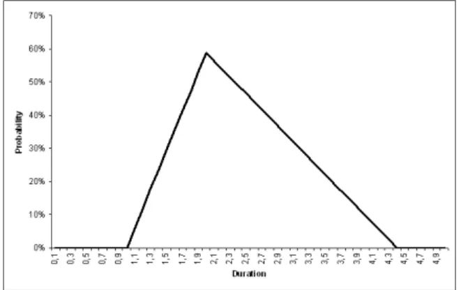
Figure 7: The impact of bad weather as a triangular distribution
Figure 8: Triangular distribution function ford10
proposed in this paper was applied. Estimates of probability and impact of both a best and worst case scenario and the overall frequency of risk occurrence were obtained from the project management team during an interview session. The obtained data were entered in a GUI1, such as shown in Figure 4. The estimates were transformed into a distribution function of the impact of risks per time unit or per activity.
Figure 7 shows the distribution function f(x) of the delays on the activity groupConcrete pouring and polishing due to bad weather conditions. A similar approach supplied the distribution functions of the impact of the other risks on the activity group.
The impact of all the concerning risks were mapped on the individual project activities. By simulating a large number of project executions (1000 iterations), a range of estimates for the realized activity duration d10 was obtained. The
dashed line in Figure 8 shows the simulated distribution function of these esti-mates. The full line represents the fitted triangular distributionf(d10). From
this triangular distribution, three estimates ofd10were distilled: respectively an
optimistic estimatea10= 1.6, a pessimisticb10= 5.3 and a most likely estimate
c10= 2.
The flexibility of activities. The project manager used the GUI to enter the activity weights using a slider bar as shown in Figure 3. The slider bar indicates that theConcrete pouring and polishing activity group was to be considered as rather flexible. This was mainly due to the fact that the activity had to be done by the company’s sufficiently available own workforce. It was expected that rescheduling this activity could be easily done without causing any major problems.
Project schedules. Multiple candidate schedules were generated for the project using the average activity durations obtained from the simulated distribution.
Four procedures were used to construct a baseline schedule: the standard resource levelling scheduling mechanism embedded in MS ProjectR, the default
ProChainR scheduling mechanism that uses the critical chain approach
(Gol-dratt (1997)) relying on the 50% rule for sizing both the feeding and project buffers. Additionally we used the ProChainR scheduling mechanism that uses
buffer sizing based on the sum of squares of both critical chain and feeding chains (see Eq. (12)), in whichndenotes the number of activities on the criti-cal chain or feeding chain,lk represents the low risk value for the duration of
activitykwhich corresponds to the 90th percentile of its duration distribution, andE(dk) corresponds to the average duration of activityk. Finally we use the
STC procedure proposed by Van de Vonder et al. (2005) and discussed above in Section 2.2., based on a 99% service level, i.e. a 99% certainty that the project delivery date will be met.
1Remark that this graphical user interface provides functionalities such as cost analysis tools that are not discussed in this work
Buffer = v u u t n X k=1 ((lk−E(dk)) 2 ) 2 (12)
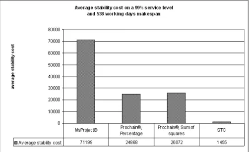
In a first analysis we took the four generated baseline schedules as input and submitted them to disruptions in 100 simulation runs of the project, using the estimated activity distributions and imposing a reactive scheduling procedure at schedule breakage that applies a robust parallel generation scheme based on a priority list that orders the activities in non-decreasing order of their starting times in the baseline schedule (Van de Vonder et al. (2006a)). The requested service level for each of the four schedules was set to 99%, which corresponds to a requested completion within 538 working days.
The results are shown in Figure 9. The results clearly demonstrate the superiority of the STC algorithm which convincingly reduces the stability costs, without compromising makespan performance.
Figure 9: Average Stability Cost
A second analysis was performed upon completion of the project. At the time when the actual disturbances that occurred during the execution of the project were all known, we confronted the four baseline schedules with the actual schedule disruptions. Each time a schedule was disrupted, the same reactive procedure as used in the first analysis, was used to repair the schedule.
Figures 11, 12 and 13 provide the Gantt charts showing only the inflexible activities of the project. The black bars represent the activities as actually performed in the actually realized project schedule. The white bars represent
the project activities as they were a priori planned in the baseline schedule. As can be seen, the unprotected schedule generated by MS ProjectR was subject to
many schedule breakages and heavy due date violation, while the STC schedule perfectly meets its due date, exhibiting a striking robustness, especially for the heavy weighted inflexible project activities.
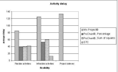
Figure 10: Average activity delays
Algorithm Kick off Planned Delivery date Stability Cost delivery date MS ProjectR 19/03/2004 25/10/2005 07/03/2006 168265 ProChainR, 19/03/2004 01/03/2007 01/03/2006 57561 Percentage ProChainR, 19/03/2004 24/04/2006 01/03/2006 64341 Sum of squares STC 19/03/2004 12/04/2006 05/04/2006 16749
Table 1: Schedule performances
Figure 10 shows that the STC algorithm efficiently protects those activities that are hard to reschedule. In other words, it perfectly meets the project due date and delivers a high solution robustness. One of the most important strengths of the STC algorithm is that it concentrates its schedule protection on those activities where stability pays off, i.e. the inflexible activities for which rescheduling is very costly. The flexible activities, where schedule stability is not
that important, are scheduled in a way that balances stability with makespan performance.
Table 1 summarizes the results of the second analysis where the four schedu-ling procedures where confronted with the disruptions that actually occurred. The schedule generated by MS ProjectR sets a completely unrealistic planned
project delivery date, which was violated by more than four months. Moreover, it suffered from numerous schedule breakages during project execution, resulting in the highest stability cost. A highly undesirable situation.
The schedule generated by ProChainR using the 50% buffer sizing rule,
included too much protection, resulting in an unacceptable planned project delivery date, caused by the insertion of a much too long project buffer. It is highly questionable whether such a long project buffer would be acceptable within the construction industry. Actually the project could be completed a year earlier than originally planned, but the schedule was subject to numerous distortions, resulting into high stability costs.
The ProChainR schedule, based on the sum of squares buffer sizing rule,
does away with the unacceptable large project buffer, but still does not clearly beat the STC algorithm on makespan. It is outperformed by the STC schedule on makespan performance and stability cost.
The STC schedule finishes the project about a month later than the other schedules. This result should be interpreted with sufficient care. Because in our model we do not take in account the possible additional delays caused by the rescheduling of activities, the shown delivery dates are likely to suffer from an underestimation. This is why it is reasonable to suspect that the additional delay caused by rescheduling inflexible activities could argue in favour of the STC algorithm. For a similar delivery date performance, the stability costs for the ProChainR and MS ProjectR schedules are much higher.
4
Conclusions
The introduction of a user friendly, time saving risk assessment method and risk database can persuade the construction project teams to go for a more quantitative risk management approach. It enables them to reuse previous risk assessments and hereby avoid recurring, time consuming efforts.
The efficient risk quantification method introduced in this paper, yields a duration distribution for each project activity. This information can accordingly be used by a proactive scheduling algorithm to insert time buffers in such a way that the planned starting time of the activities and the realization time of the milestones that suffer from a high disruption cost, are sufficiently protected. Unlike ProChainR and MS ProjectR, the STC algorithm schedules the activities
to such extent that both solution and quality robustness are boosted, without giving in on makespan performance.
The results obtained during the implementation of the methodology on real life projects are very promising. Further research will refine the risk database and hopefully allow the construction companies to reap the benefits of increased
References
Al-Bahar, J. and Crandall, K. (1990). Systematic risk management approach for construction projects. Journal of Construction Engineering and Man-agement, 116, pp 533–546.
Assaf, S. and Al-Hejji, S. (2006). Causes of delay in large construction projects.
International Journal of Project Management, 24, pp 349–357.
Ben-David, I. and Raz, T. (2001). An integrated approach for risk response de-velopment in project planning.Journal of the Operational Research Society, 52, pp 14–25.
Carr, V. and Tah, J. (2001). A fuzzy approach to construction project risk assessment and analysis: construction project risk management system.
Advances in Engineering Software, 32, pp 847–857.
Chapman, C. and Ward, S. (2000). Estimation and evaluation of uncertainty: A minimalist first pass approach. International Journal of Project Man-agement, 18, pp 369–383.
Choi, H., Cho, H. and Seo, J. (2004). Risk assessment methodology for un-derground construction projects.Journal of Construction Engineering and Management, 130, pp 258–272.
Demeulemeester, E. and Herroelen, W. (2002). Project scheduling - A research handbook. Vol. 49 ofInternational Series in Operations Research & Man-agement Science. Kluwer Academic Publishers, Boston.
Edwards, P. and Bowen, P. (2000). Risk and risk management in construc-tion projects: Concepts, terms and risk categories re-defined. Journal of Construction Procurement, (5), pp 42–57.
Elmaghraby, S., Herroelen, W. and Leus, R. (2003). Note on the paper ’resource-constrained project management using enhanced theory of constraints’.
International Journal of Project Management, 21, pp 301–305.
Goldratt, E. (1997). Critical Chain. The North River Press Publishing Corpo-ration, Great Barrington.
Herroelen, W. (2005). Project scheduling - theory and practice.Production and Operations Management, 14, pp 413–432.
Herroelen, W., De Reyck, B. and Demeulemeester, E. (1998). Resource-constrained scheduling: a survey of recent developments. Computers and Operations Research, 25, pp 279–302.
Herroelen, W. and Leus, R. (2001). On the merits and pitfalls of critical chain scheduling.Journal of Operations Management, 128(3), pp 221–230.
Herroelen, W. and Leus, R. (2004). Robust and reactive project scheduling: a review and classification of procedures.International Journal of Production Research, 42(8), pp 1599–1620.
Herroelen, W. and Leus, R. (2005). Project scheduling under uncertainty – Survey and research potentials.European Journal of Operational Research, 165, pp 289–306.
Herroelen, W., Leus, R. and Demeulemeester, E. (2002). Critical chain project scheduling: Do not oversimplify. Project Management Journal, 33, pp 48– 60.
Jannadi, O. and Almishari, S. (2003). Risk assessment in construction.Journal of Construction Engineering and Management, 129, pp 492–500.
Leus, R. and Herroelen, W. (2005). The complexity of machine scheduling for stability with a single disrupted job. Operations Research Letters, 33, pp 151–156.
Lyons, T. and Skitmore, M. (2004). Project risk management in the queens-land engineering construction industry: a survey.International Journal of Project Management, 22, pp 55–61.
Maes, J., Vandoren, C., Sels, L. and Roodhooft, F. (2006). Onderzoek naar oorzaken van faillissementen van kleine en middelgrote bouwondernemein-gen. Research report. Department of applied economics, Katholieke Uni-versiteit Leuven, Belgium.
Mulholland, B. and Christian, J. (1999). Risk assessment in construction sche-dules.Journal of Construction Engineering and Management, 125, pp 8–15. Newbold, R. (1998).Project management in the fast lane - Applying the Theory of Constraints. APICS Series on Constraints Management. The St. Lucie Press.
Oglesby, C., Parker, H. and Howell, G. (1989). Productivity improvement in construction. McGraw-Hill, New York.
Park, M. and Pea-Mora, F. (2004). Reliability buffering for construc-tion projects. Journal of Construction Engineering and Management, 130, pp 626–637.
PMI (2000). A Guide to the Project Management Body of Knowledge. Project Management Institute, Newton Square.
Tukel, O., Rom, W. and Eksioglu, S. (2006). An investigation of buffer sizing techniques in critical chain scheduling. European Journal of Operational Research, 172, pp 401–416.
Van de Vonder, S. (2006). Proactive/reactive procedures for robust project scheduling. PhD thesis. Research Center for Operations Management, Katholieke Universiteit Leuven, Belgium.
Van de Vonder, S., Ballestin, F., Demeulemeester, E. and Herroelen, W. (2006a). Heuristic procedures for reactive project scheduling.Computers and Indus-trial Engineering, . to appear.
Van de Vonder, S., Demeulemeester, E. and Herroelen, W. (2005). An investiga-tion of efficient and effective predictive-reactive project scheduling proce-dures.Research Report 0466. Department of applied economics, Katholieke Universiteit Leuven, Belgium.
Van de Vonder, S., Demeulemeester, E., Herroelen, W. and Leus, R. (2005a). The use of buffers in project management: the trade-off between stability and makespan.International Journal of Production Economics, 97, pp 227– 240.
Van de Vonder, S., Demeulemeester, E., Herroelen, W. and Leus, R. (2006). The trade-off between stability and makespan in resource-constrained project scheduling.International Journal of Production Research, 44, pp 215–236. Warszawski, A. and Sacks, R. (2004). Practical multifactor approach to eval-uating risk of investment in engineering projects. Journal of Construction Engineering an Management, 130, pp 357–367.