Options trading driven by volatility directional
accuracy
Maris, Konstantinos Michael; Nikolopoulos, Konstantinos; Giannelos,
Konstantinos George; Assimakopoulos, Vassilis
Postprint / Postprint
Zeitschriftenartikel / journal article
Zur Verfügung gestellt in Kooperation mit / provided in cooperation with: www.peerproject.eu
Empfohlene Zitierung / Suggested Citation:
Maris, Konstantinos Michael ; Nikolopoulos, Konstantinos ; Giannelos, Konstantinos George ; Assimakopoulos, Vassilis: Options trading driven by volatility directional accuracy. In: Applied Economics 39 (2006), 2, pp. 253-260. DOI:
http://dx.doi.org/10.1080/00036840500427999
Nutzungsbedingungen:
Dieser Text wird unter dem "PEER Licence Agreement zur Verfügung" gestellt. Nähere Auskünfte zum PEER-Projekt finden Sie hier: http://www.peerproject.eu Gewährt wird ein nicht exklusives, nicht übertragbares, persönliches und beschränktes Recht auf Nutzung dieses Dokuments. Dieses Dokument ist ausschließlich für den persönlichen, nicht-kommerziellen Gebrauch bestimmt. Auf sämtlichen Kopien dieses Dokuments müssen alle Urheberrechtshinweise und sonstigen Hinweise auf gesetzlichen Schutz beibehalten werden. Sie dürfen dieses Dokument nicht in irgendeiner Weise abändern, noch dürfen Sie dieses Dokument für öffentliche oder kommerzielle Zwecke vervielfältigen, öffentlich ausstellen, aufführen, vertreiben oder anderweitig nutzen.
Mit der Verwendung dieses Dokuments erkennen Sie die Nutzungsbedingungen an.
Terms of use:
This document is made available under the "PEER Licence Agreement ". For more Information regarding the PEER-project see: http://www.peerproject.eu This document is solely intended for your personal, non-commercial use.All of the copies of this documents must retain all copyright information and other information regarding legal protection. You are not allowed to alter this document in any way, to copy it for public or commercial purposes, to exhibit the document in public, to perform, distribute or otherwise use the document in public.
By using this particular document, you accept the above-stated conditions of use.
For Peer Review
Options trading driven by volatility directional accuracy
Journal: Applied Economics
Manuscript ID: APE-05-0251.R1 Journal Selection: Applied Economics Date Submitted by the
Author: 15-Aug-2005
JEL Code: C10 - General < , C22 - Time-Series Models < , C45 - Neural Networks and Related Topics < , G15 - International Financial Markets <
For Peer Review
Options trading driven by volatility directional accuracy
Abstract
Analysts have claimed over the last years that the volatility of an asset is caused solely by the random arrival of new information about the future returns from the underlying asset. It is a common belief that volatility is of great importance in finance and it is one of the critical factors determining option prices and consequently driving option-trading strategies. This paper discusses an empirical option trading methodology based on efficient volatility direction forecasts. Although in most cases accurate volatility forecasts are hard to obtain, forecasting the direction is significantly easier. Increase in the directional accuracy leads to profitable investment strategies. The net gain is depended on the size of the changes as well; however successful volatility forecasts in terms of directional accuracy was found to be sufficient for positive results. In order to evaluate the proposed methodology weekly data from CAX40, DAX and the Greek FTSE/ASE 20 stock indices were used.
Keywords: Decision Support, Options Trading, Forecasting, Volatility, Directional Accuracy 3 4 5 6 7 8 9 10 11 12 13 14 15 16 17 18 19 20 21 22 23 24 25 26 27 28 29 30 31 32 33 34 35 36 37 38 39 40 41 42 43 44 45 46 47 48 49 50 51 52 53 54 55 56 57 58
For Peer Review
1. IntroductionEfficient valuation of options is of crucial importance for practitioners in any financial market (Chen and Leung 2003, Yoshida 2003, Andersen 2002, Buckley et. al 2002, Grace 2000, Pedersen 1998). Options during the last decade became a key component in the majority of investment portfolios. This development is reflected by the fact that both the turnover and the volume of these products have experienced phenomenal growth since the 1970s (Bjork 1998).
Option pricing is based on a variety of factors. From the main components that affect the premium of an option the only component that cannot be observed directly is the volatility of the underlying asset. Volatility measures the amount by which an underlying asset is expected to fluctuate in a given period of time. It significantly impacts the price of an option’s premium and heavily contributes to an option’s time value (Hull 1997).
Volatility can be viewed as the speed of change in the price of the underlying instrument. The higher the volatility, the more chance an option has of becoming profitable by expiration. Reviewing volatility levels can help traders determine the right option strategy (Caner and Onder 2005, Bautista 2005, Kim et al. 2004, Fofana and Brorsen 2001, Bautista 2003, Arago-Manzana and Fernandez-Izquierdo 2003, Bahmani-Oskooee 2002). Forecasting financial market volatility has absorbed the interest of many academics in the last decade (Sabanis 2002, Fouque et. al 2001, Skiadopoulos 2001, Lux and Marchesi 2000).
3 4 5 6 7 8 9 10 11 12 13 14 15 16 17 18 19 20 21 22 23 24 25 26 27 28 29 30 31 32 33 34 35 36 37 38 39 40 41 42 43 44 45 46 47 48 49 50 51 52 53 54 55 56
For Peer Review
The present study discusses an empirical option trading methodology based on volatility direction forecasts. Although in most cases accurate volatility forecasts are hard to obtain (Maris et. al 2004a), forecasting the direction is a bit easier. Increase in the directional accuracy leads to profitable investment strategies. The net gain is always depended on the size of the changes as well, however accuracy over 60% was found to guarantee profitable investment. In order to evaluate the proposed methodology weekly data from CAX, DAX and the Greek FTSE/ASE 20 stock indices were used. This study builds on earlier results presented in a study with data from the Greek market (Maris et. al 2004b) where volatility point forecasts were produced with the Theta model (Nikolopoulos and Assimakopoulos 2003, Assimakopoulos and Nikolopoulos 2000).
The study is structured as follows: the next section aims to introduce the reader to the options. In section three the options trading methodology is presented, while in the fourth section follows an evaluation in both terms of volatility directional accuracy and investment revenue. The last section summarizes the conclusions and future research.
2. Options
Options confer upon the holder the right to buy or sell an asset in the future for a given price. There are two basic types of options: A Call (C) gives the holder the right to buy while a Put (P) gives the holder the right to sell. The price at which the future transaction may be carried out is known as the strike price or exercise price.
3 4 5 6 7 8 9 10 11 12 13 14 15 16 17 18 19 20 21 22 23 24 25 26 27 28 29 30 31 32 33 34 35 36 37 38 39 40 41 42 43 44 45 46 47 48 49 50 51 52 53 54 55 56 57 58
For Peer Review
There are two sides to every option contract. On one side is the investor who has taken the long position (has bought the option) and on the other side is the investor who has taken the short position (has sold or written the option). The writer of the option receives cash upfront but has potential liabilities later. In order to ensure that writers of calls and puts are able to honour their obligations to sell or buy the underlying item, writers have to make a security deposit (margin). The net margin is calculated daily on the basis of the client’s options and futures account. The important feature of options is that they do not have to be exercised (Hull 1997).
There are numerous strategies available for taking advantage of increases or decreases in volatility. These strategies are called non-directional strategies or volatility strategies. They are delta neutral strategies, where delta ( ) is one of the sensitivity factors that measure how an option’s value changes with respect to a change in the price of the underlying asset (Hull 1997). Volatility is subject to the forces of supply and demand. As a result volatility will tend to rise during periods when demand from options buyers is strongest and will fall when demand is weakest.
Various delta neutral strategies have been proposed in the bibliography (Hull 1997, Briys et al. 1998, McMillan 2002): Long & Short Straddle, Long & Short Strangle, Call & Put Back Spread, Call & Put Ratio Spread, Long & Short Butterfly, Long & Short Call Christmas tree, Long & Short put Christmas tree. These strategies involve different levels of risk.
[INSERT FIGURE 1 ABOUT HERE] 3 4 5 6 7 8 9 10 11 12 13 14 15 16 17 18 19 20 21 22 23 24 25 26 27 28 29 30 31 32 33 34 35 36 37 38 39 40 41 42 43 44 45 46 47 48 49 50 51 52 53 54 55 56
For Peer Review
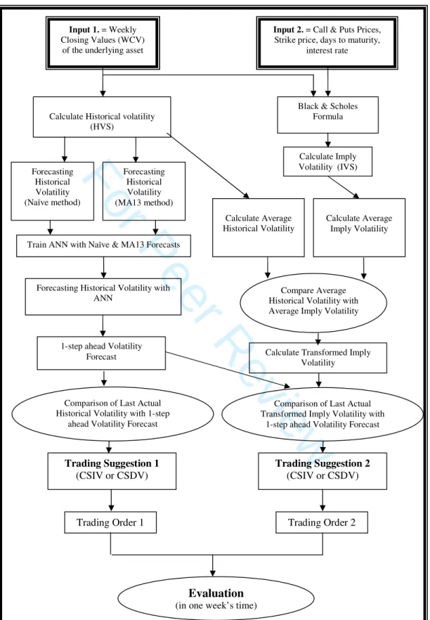
3. Options Trading MethodologyThe proposed options trading methodology is consisted of a number of necessary sequential steps in order to reach an investment decision, as presented in figure 1 and analysed below:
Weekly Closing Values (WCV) of the underlying instrument are obtained from the relevant markets. A new value is inserted each period to the database in order to update the time series.
From WCV series two volatility (annual) series are calculated, the Historical Volatility Series (HVS) and the Imply Volatility Series (IVS) where the Black & Scholes formula is used (Hull 1997).
One step-ahead forecast is produced for HVS with two different extrapolating methods. The Naïve method that performs very well for short-term forecasting and a Moving Average of thirteen periods- MA13 (13 weeks = one term) that performs well for the medium-term (Assimakopoulos and Vafopoulos 2000). A two-layer Artificial Neural Network (ANN) is trained with the Back-propagation algorithm (Haykin 1998) to combine these forecasts in order to produce as accurate forecasts as possible in terms of directional accuracy. We are interested in getting right the direction for the next period rather than the actual value itself. So we combine two point forecasts from different approaches (one short-term and one medium-term oriented) in order to get one efficient forecast for the direction of the series. The directional accuracy of the combination is better than the directional accuracy of the two methods that are weighted by the ANN (Naïve and MA13). In order to produce profitable investments accuracy over the threshold of 60% should be achieved. It must 3 4 5 6 7 8 9 10 11 12 13 14 15 16 17 18 19 20 21 22 23 24 25 26 27 28 29 30 31 32 33 34 35 36 37 38 39 40 41 42 43 44 45 46 47 48 49 50 51 52 53 54 55 56 57 58
For Peer Review
be noted that the majority of Academics in the forecasting field are in favour of combining, a empirical principle that was also verified in the largest ever forecasting competition, the M3-competition (Makridakis and Hibon 2000); an equal weighted combination of three exponential smoothing approaches outperformed the performance of each method separately. However it is not always the case that a combination can outperform any individual method, as proved by the performance of the Theta model - a single univariate method that outperformed all combinations in the very same competition (Assimakopoulos and Nikolopoulos, 2000). Overall we are in favour of the combinatory approach in this study as it comes for the minimisation of risk as well as the usually increased accuracy.
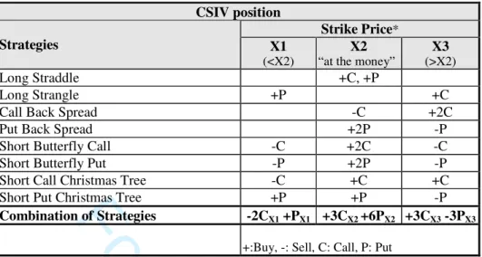
The one step-ahead forecast is then compared with the last actual value of the two volatility series HVS and IVS. In some cases IVS has to be transformed so as to be in the same level (mean) with HVS and make comparisons feasible. If the forecast is greater than the last observed actual then the trader is adopting a Combination of Strategies for Increasing Volatility (CSIV), otherwise a Combination of Strategies for Decreasing Volatility (CSDV) is taken. These two sets of positions CSIV & CSDV are explained in detail in table 1. Since there are two volatility series, two comparisons are made and consequently two trading suggestions are produced. In the case that the trading suggestions are in the opposite direction (the HVS series comparison suggest CSIV positioning while the IVS series a CSDV one or vice versa) then no action is made at all for this period and the trader waits for the next period.
[INSERT TABLE 1 ABOUT HERE] 3 4 5 6 7 8 9 10 11 12 13 14 15 16 17 18 19 20 21 22 23 24 25 26 27 28 29 30 31 32 33 34 35 36 37 38 39 40 41 42 43 44 45 46 47 48 49 50 51 52 53 54 55 56
For Peer Review
Thus, the CSIV trading order is consisted of two Short Calls (selling two buying options) and one Long Put (buying one selling option) with strike price lower than the “at the money” price of the underlying asset, three Long Calls and six Long Puts “at the money”, and three Long Calls and three Short Puts with strike price greater than the “at the money” price. The maximum profit from this portfolio is infinite while the maximum loss is: r = (P X1+3C X2+6P X2+3C X3)-(3P X3+2CX1).
On the other hand CSDV is exactly the complimentary position where this time as expected the maximum loss is infinite and the maximum profit equal to r.
4. Evaluation
The proposed methodology was evaluated based on the directional accuracy of volatility forecasts, as well as the financial success of the trading suggestions.
4.1 Directional accuracy
The time-series under consideration consist of weekly observations (Friday closing values) from three stock indices: CAC40, DAX and the Greek FTSE20. All three series stand for annual volatility (calculated on the relative underlying stock indices, Hull 1997). The graph of the DAX series follows in figure 2. The sample period of the time-series under examination covers 238 weeks. The first 212 weekly observations were used for the estimation of the models’ parameters, from the period starting on the 27/08/1999 to the period ending on the 17/10/2003 (weeks t: 1, 2, ... 212). The authors held out the last 26 observations (weeks t: 213, … 238) up to the period ending on the 16/4/2004, in order to evaluate the models out of sample one–step-ahead forecasting accuracy. Thus, the average out of sample forecasting accuracy was calculated over 26 one-step-ahead errors.
3 4 5 6 7 8 9 10 11 12 13 14 15 16 17 18 19 20 21 22 23 24 25 26 27 28 29 30 31 32 33 34 35 36 37 38 39 40 41 42 43 44 45 46 47 48 49 50 51 52 53 54 55 56 57 58
For Peer Review
The rational behind the choice of such a small holdout (relatively to the length of the series) comes from a financial economics perspective. The trading strategy should be able to be compared with actual yearly or 6-months bonds and investment portfolios; that is why 26 weeks were selected, however 52 weeks could be an alternative holdout. In terms of the standard practise in forecasting literature (Makridakis et al. 1998), usually holdouts of about 20% - 40% of the series are selected; however this is the practice in blind competitions, where the source of the data is unknown and holdouts of specific length do not make any real difference.
[INSERT FIGURE 2 ABOUT HERE]
Assimakopoulos and Vafopoulos (2000) conducted an extensive survey of available forecasting techniques for stock market volatility. In the present study a forecasting competition was conducted with eleven different approaches from that study: the random walk model (NAÏVE); the mean model (MEAN); the exponential smoothing model (SES) (Makridakis et al., 1998); Moving Averages of 4, 8, 13 and 26 weeks (MA4, MA8, MA13, MA26); and four models from the ARCH family (ARCH, GARCH, EGARCH, TARCH) (Alexander, 1999).
Those methods were proven inadequate for the Greek market in an earlier study (Maris et al. 2004a). Having in mind that the financial evaluation is going to be conducted only in the Greek Market where detailed data are available, the authors decided to used ANN as mentioned earlier in order to combine the forecasts from some of these simpler approaches.
3 4 5 6 7 8 9 10 11 12 13 14 15 16 17 18 19 20 21 22 23 24 25 26 27 28 29 30 31 32 33 34 35 36 37 38 39 40 41 42 43 44 45 46 47 48 49 50 51 52 53 54 55 56
For Peer Review
Instead of challenging the forecasting accuracy of these models in terms of point-forecasts oriented error metrics (RMSE or MAPE, Makridakis et al. 1998) the authors decided to use Directional Accuracy measures. The rational behind this decision is twofold: First it is much easier to forecast whether volatility is going to increase or decrease rather than estimating a point forecast, and secondly the trading strategies that will be used are based on the sign of the volatility change.
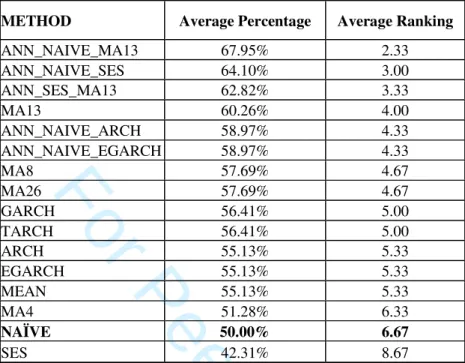
The directional accuracy is measured as a percentage of the times you get right the direction of the volatility forecast divided by the times you make a forecast. For our research we conducted 26 forecasts for each Stock Market. So the Average Percentage is calculated as the ratio of the successful volatility direction over the 72 attempts across the three different markets. The average ranking is calculated a bit differently. The methods are ranked for each separate market according to their directional accuracy and then an average of these three positions is taken. The combination from an ANN of forecasts from the NAIVE method and MA13 proved to be the best with both average measures (Table 2, Average Percentage 67.95% and Average Ranking 2.33) as a result of taking the first place in CAC40 (Directional Accuracy 80.77%), the fourth place in DAX (Directional Accuracy 57.69%) and the second place in FTSE20 (Directional Accuracy 65.38%). The NAÏVE method provides by definition 50% directional accuracy as it does not provide sign.
[INSERT TABLE 2 ABOUT HERE] 3 4 5 6 7 8 9 10 11 12 13 14 15 16 17 18 19 20 21 22 23 24 25 26 27 28 29 30 31 32 33 34 35 36 37 38 39 40 41 42 43 44 45 46 47 48 49 50 51 52 53 54 55 56 57 58
For Peer Review
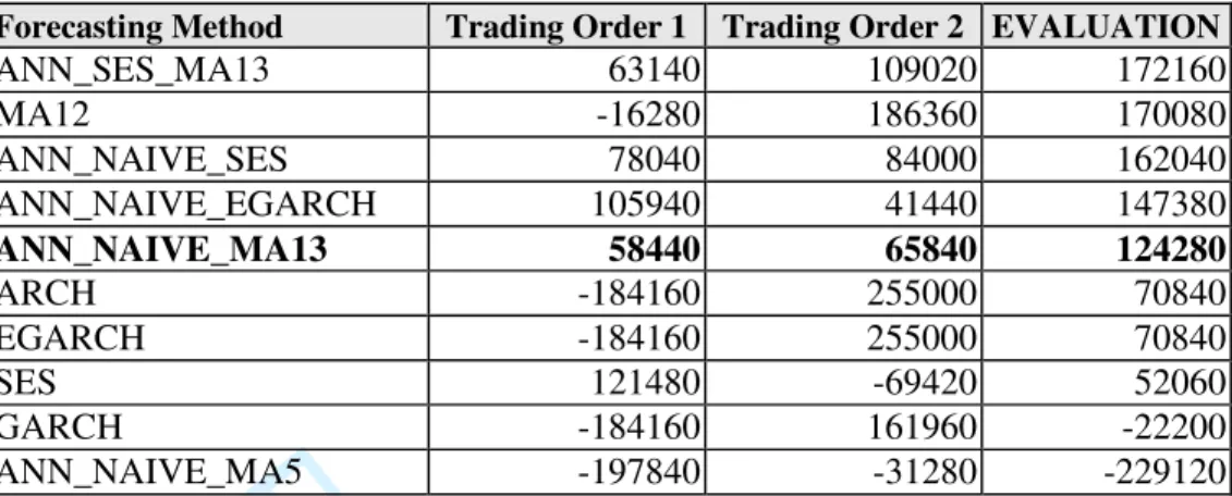
4.2 Position EvaluationIn order to evaluate the proposed trading methodology, we made transactions of 100 contracts on the FTSE/ASE 20 index in a period of 26 weeks (six months), from the 24/10/2003 to 16/4/2004. The index multiplier is 5. The cost of a contract in Euros is given by multiplying the price with the index multiplier. A week later we closed our positions by taking the opposite positions no mater if we had a loss or a profit. Similarly we conducted transactions with directional forecasts form other forecasting approaches over 26 weeks and computed the total profit/loss of our positions. The results of this real-data simulation are shown in Table 3.
[INSERT TABLE 3 ABOUT HERE]
All the results presented in table 3 are extracted using the same trading strategy. The only difference in each case is the method that produced the forecasts for the direction of the volatility. It is clear that the best method (ANN_NAÏVE_MA13) in terms of directional accuracy did not produce the best financial results. However it produced better financial results than established methods (as the ARCH family) and better results than all the simple methods with the exception of the moving average of twelve weeks
This result was partially expected, as a successful directional forecast does not guarantee maximisation of the profit. This is due to the fact that one successful forecast for only one period could cause major profit, more than two or three other successful forecasts. This has to do with the fact that not only the direction counts but the size of the volatility moves as well. Thus, the next step of the methodology should be to find the best method in terms of directional accuracy percentage but restricted to 3 4 5 6 7 8 9 10 11 12 13 14 15 16 17 18 19 20 21 22 23 24 25 26 27 28 29 30 31 32 33 34 35 36 37 38 39 40 41 42 43 44 45 46 47 48 49 50 51 52 53 54 55 56
For Peer Review
those directional moves sized over a certain threshold i.e. 5%; those that resulted in having a large profit. Nevertheless, the fact that the proposed methodology was profitable over a period of half a year, with 26 continuous trades, is by all means very promising.
5. Conclusion
This study presented an empirical option trading methodology based on forecasts for the direction of the volatility of the underlying financial index. The proposed methodology is easy to apply, easy to embed in an Information System and requires standard inputs available freely via the Internet for the majority of stock markets.
A high directional accuracy leads to profitable investment strategies, however the net end result always depends on the size of changes as well. An empirical threshold of 60% of successful volatility forecasts was found to be sufficient for creating profitability within a period of six calendar months. The proposed volatility forecasting approach was validated on weekly data obtained from CAX40, DAX and the Greek FTSE/ASE 20 stock indices while the trading strategy using data only from the Greek index.
For the production of volatility forecasts an ANN was employed in order to combine the forecasts from two simpler approaches: the short-term oriented Naïve method and the mid -term oriented Moving Average of thirteen weeks model. This method proved to perform best across the three different markets. The forecasting method is by definition more robust due to the combinatory nature.
3 4 5 6 7 8 9 10 11 12 13 14 15 16 17 18 19 20 21 22 23 24 25 26 27 28 29 30 31 32 33 34 35 36 37 38 39 40 41 42 43 44 45 46 47 48 49 50 51 52 53 54 55 56 57 58
For Peer Review
The proposed methodology produced profit for a period of six months (26 weeks). For each week the methodology provides two trading suggestions - one based on the historical volatility and another on the implied one. The robustness of the method is once more verified, as both trading orders are on average profitable over the testing period. However, while applying the same trading strategy to volatility forecasts from less accurate models, some interesting results came up; some simpler approaches produced better financial results. This was partially expected, as a successful directional forecast does not guarantee maximisation of the profit. This is due to the fact that one successful forecast for only one period could cause major profit, more than two or three other successful forecasts.
Future research should be focused towards finding the best method in terms of directional accuracy but restricted to those directional moves over a certain margin; these changes are expected to result in big profits. Also more practical issues should be addressed in order to test the methodology with more frequent data i.e. daily data or intraday data. Finally the proposed methodology should be embedded in a prototype information system in order to be widely tested in other stock markets (FTSE, DJIA, NASDAQ), and become more generic. Nevertheless, the evaluation results and the simplicity of the proposed approach make it rather attractive and by all means worth expanding.
Acknowledgement
The authors would like to thank Mr. Michael C. Handrinos from Lancaster University for his comments and suggestions in the final revision of this paper.
3 4 5 6 7 8 9 10 11 12 13 14 15 16 17 18 19 20 21 22 23 24 25 26 27 28 29 30 31 32 33 34 35 36 37 38 39 40 41 42 43 44 45 46 47 48 49 50 51 52 53 54 55 56
For Peer Review
ReferencesAlexander, C. (1999) Risk Management and Analysis, Volume 1: Measuring and Modelling Financial Risk, John Wiley & Sons, Chichester.
Arago-Manzana, V. and Fernandez-Izquierdo, M.A. (2003) Monthly seasonality of the returns and volatility of the IBEX-35 index and its futures contract, Journal of Applied Economics Letters, 10 (3), 129-133.
Andersen, L. (2002) How Options Analysis Can Enhance Managerial Performance, European Management Journal, 20(5), 505-511.
Assimakopoulos, V. and Nikolopoulos, K. (2000) The Theta model: a decomposition approach to forecasting, International Journal of Forecasting, 16 (4), 521-530. Assimakopoulos V. and Vafopoulos M. (2000) Financial Volatility Forecasting,
Economic & Financial Computing, 10 (3), Autumn.
Bahmani-Oskooee, M. (2002) Does black market exchange rate volatility deter the trade flows? Iranian experience, Applied Economics, 34 (18), 2249-2255. Bautista, C.C. (2005) How volatile are East Asian stocks during high volatility
periods?, Journal of Applied Economics Letters, 12 (5), 319-326.
Bautista, C.C. (2003) Stock market volatility in the Philippines, Journal of Applied Economics Letters, 10 (5), 315-318.
Bjork, T. (1998) Arbitrage Theory in Continuous Time, Oxford University Press, Oxford.
Briys, E., Mai, H.M., Bellalah, M. and de Varenne, F. (1998) Options, Futures and Exotic Derivatives, Theory, Application and Practice. John Wiley & Sons, Chichester. 3 4 5 6 7 8 9 10 11 12 13 14 15 16 17 18 19 20 21 22 23 24 25 26 27 28 29 30 31 32 33 34 35 36 37 38 39 40 41 42 43 44 45 46 47 48 49 50 51 52 53 54 55 56 57 58
For Peer Review
Buckley, A., Tse, K., Rijken, H. and Eijgenhuijsen, H. (2002) Stock Market Valuation with Real Options: lessons from Netscape, European Management Journal, 20 (5), 512-526.
Caner, S. and Onder, Z. (2005) Sources of volatility in stock returns in emerging markets, Applied Economics, 37 (8), 929-941.
Chen, A.S.and Leung, M.T. (2003) Option straddle trading: Financial performance and economic significance of direct profit forecast and conventional strategies, Journal of Applied Economics Letters,10 (8), 493-498.
Fofana, N.F. and Brorsen, B.W. (2001) GARCH option pricing with implied volatility, Journal of Applied Economics Letters, 8 (5), 335-340.
Fouque, J-P., Papanicolaou,G. and Sircar K.R. (2001) From the Implied Volatility Skew to a Robust Correction to Black-Scholes American Option Prices, International Journal of Theoretical and Applied Finance,4 (4), 651-675. Grace, B.K. (2000) Black-Scholes option pricing via genetic algorithms, Journal of
Applied Economics Letters, 7 (2), 129-132.
Haykin, S. (1998) Neural Networks: A Comprehensive Foundation (International Edition), Pearson US Imports & PHIPEs.
Hull, C.J. (1997) Options, Futures and Other Derivatives. (3rd Edition), Prentice Hall, London.
Kim, M.H., Kim, G.R. and Kim, M. (2004) Stock market volatility and trading activities in the KOSPI 200 derivatives markets, Journal of Applied Economics Letters, 11 (1), 49-53.
Lux, T. and Marchesi M. (2000) Volatility Clustering in Financial Markets A Microsimulation of Interacting Agents, International Journal of Theoretical and Applied Finance, 3 (4), 675-702.
McMillan, L.G. (2002) Options As a Strategic Investment (4th Edition Study Guide), Prentice Hall Press, New York.
3 4 5 6 7 8 9 10 11 12 13 14 15 16 17 18 19 20 21 22 23 24 25 26 27 28 29 30 31 32 33 34 35 36 37 38 39 40 41 42 43 44 45 46 47 48 49 50 51 52 53 54 55 56
For Peer Review
Makridakis S. and Hibon, M., (2000), The M3-Competition: Results, conclusions and implications, International Journal of Forecasting 16, pp. 451-476.
Makridakis, S., Wheelwright, S., & Hyndman, R., (1998). Forecasting Methods and Applications. (3rd Edition), John Wiley & Sons, New York.
Maris, K., Pantou, G., Nikolopoulos, K., Pagourtzi, E. and Assimakopoulos, V. (2004a) A study of financial volatility forecasting techniques in the FTSE/ASE 20 index, Journal of Applied Economics Letters, 11 (7), 453-457.
Maris, K., Metaxiotis, K., Pantou, G., Nikolopoulos, K., Tavanidou, E. and Assimakopoulos, V. (2004b) D-TIFIS: A decision support system for options trading, Information Management & Computer Security, 12 (1), 45-65.
Merton, R. C., (1973) Theory of Rational Option Pricing, Bell Journal of Economics, 4 (1), 141-183.
Natenberg S. (1994) Option Volatility & Pricing: Advanced Trading Strategies and Techniques, 2nd edition, Mc Graw Hill.
Nikolopoulos, K. and Assimakopoulos, V. (2003) Theta Intelligent Forecasting Information System, Industrial Management and Data Systems, 103 (9), 711-726.
Pedersen, W.R. (1998) Capturing all the information in foreign currency option prices: solving for one versus two implied variables, Applied Economics, 30 (12), 1679-1683.
Skiadopoulos, G. (2001) Volatility Smile consistent Option Models A Survey, International Journal of Theoretical and Applied Finance, 4 (3), 403-437. Sabanis, S. (2002) Stochastic Volatility, International Journal of Theoretical and
Applied Finance,5 (5) 515-530.
Yoshida, Y. (2003) The valuation of European options in uncertain environment, European Journal of Operational Research, 145 (1), 221-229.
3 4 5 6 7 8 9 10 11 12 13 14 15 16 17 18 19 20 21 22 23 24 25 26 27 28 29 30 31 32 33 34 35 36 37 38 39 40 41 42 43 44 45 46 47 48 49 50 51 52 53 54 55 56 57 58
For Peer Review
Figure 1. Flow diagram for the proposed methodology.Comparison of Last Actual Transformed Imply Volatility with
1-step ahead Volatility Forecast Train ANN with Naïve & MA13 Forecasts
1-step ahead Volatility Forecast Input 1. = Weekly Closing Values (WCV)
of the underlying asset
Input 2. = Call & Puts Prices, Strike price, days to maturity,
interest rate Calculate Imply Volatility (IVS) Trading Suggestion 1 (CSIV or CSDV) Trading Order 1
Comparison of Last Actual Historical Volatility with 1-step
ahead Volatility Forecast
Compare Average Historical Volatility with Average Imply Volatility
Calculate Transformed Imply Volatility
Trading Suggestion 2 (CSIV or CSDV)
Trading Order 2
Evaluation (in one week’s time)
Forecasting Historical Volatility with ANN Forecasting Historical Volatility (Naïve method) Forecasting Historical Volatility (MA13 method) Calculate Historical volatility
(HVS)
Black & Scholes Formula
Calculate Average
Historical Volatility Calculate Average Imply Volatility
3 4 5 6 7 8 9 10 11 12 13 14 15 16 17 18 19 20 21 22 23 24 25 26 27 28 29 30 31 32 33 34 35 36 37 38 39 40 41 42 43 44 45 46 47 48 49 50 51 52 53 54 55 56
For Peer Review
Table 1. Combination of Strategies for Increasing Volatility (CSIV)
CSIV position
Strike Price*
Strategies X1
(<X2) “at the money” X2 (>X2) X3
Long Straddle +C, +P
Long Strangle +P +C
Call Back Spread -C +2C
Put Back Spread +2P -P
Short Butterfly Call -C +2C -C
Short Butterfly Put -P +2P -P
Short Call Christmas Tree -C +C +C
Short Put Christmas Tree +P +P -P
Combination of Strategies -2CX1 +PX1 +3CX2 +6PX2 +3CX3 -3PX3
+:Buy, -: Sell, C: Call, P: Put 3 4 5 6 7 8 9 10 11 12 13 14 15 16 17 18 19 20 21 22 23 24 25 26 27 28 29 30 31 32 33 34 35 36 37 38 39 40 41 42 43 44 45 46 47 48 49 50 51 52 53 54 55 56 57 58
For Peer Review
Figure 2. Annual volatility (calculated on the German DAX stock index)
0 20 40 60 80 100 3 4 5 6 7 8 9 10 11 12 13 14 15 16 17 18 19 20 21 22 23 24 25 26 27 28 29 30 31 32 33 34 35 36 37 38 39 40 41 42 43 44 45 46 47 48 49 50 51 52 53 54 55 56
For Peer Review
Table 2. CAC40, DAX, FTSE20 - Directional Accuracy (Rolling over 26 one-week ahead forecasts)
METHOD Average Percentage Average Ranking
ANN_NAIVE_MA13 67.95% 2.33 ANN_NAIVE_SES 64.10% 3.00 ANN_SES_MA13 62.82% 3.33 MA13 60.26% 4.00 ANN_NAIVE_ARCH 58.97% 4.33 ANN_NAIVE_EGARCH 58.97% 4.33 MA8 57.69% 4.67 MA26 57.69% 4.67 GARCH 56.41% 5.00 TARCH 56.41% 5.00 ARCH 55.13% 5.33 EGARCH 55.13% 5.33 MEAN 55.13% 5.33 MA4 51.28% 6.33 NAÏVE 50.00% 6.67 SES 42.31% 8.67 3 4 5 6 7 8 9 10 11 12 13 14 15 16 17 18 19 20 21 22 23 24 25 26 27 28 29 30 31 32 33 34 35 36 37 38 39 40 41 42 43 44 45 46 47 48 49 50 51 52 53 54 55 56 57 58
For Peer Review
Table 3. Position evaluation over 26 weeks in Euros (FTSE20)
Forecasting Method Trading Order 1 Trading Order 2 EVALUATION
ANN_SES_MA13 63140 109020 172160 MA12 -16280 186360 170080 ANN_NAIVE_SES 78040 84000 162040 ANN_NAIVE_EGARCH 105940 41440 147380 ANN_NAIVE_MA13 58440 65840 124280 ARCH -184160 255000 70840 EGARCH -184160 255000 70840 SES 121480 -69420 52060 GARCH -184160 161960 -22200 ANN_NAIVE_MA5 -197840 -31280 -229120 3 4 5 6 7 8 9 10 11 12 13 14 15 16 17 18 19 20 21 22 23 24 25 26 27 28 29 30 31 32 33 34 35 36 37 38 39 40 41 42 43 44 45 46 47 48 49 50 51 52 53 54 55 56