OpenBU http://open.bu.edu
Theses & Dissertations Boston University Theses & Dissertations
2015
Local learning by partitioning
https://hdl.handle.net/2144/15204 Boston University
COLLEGE OF ENGINEERING
Dissertation
LOCAL LEARNING BY PARTITIONING
by
JOSEPH WANG
B.S., Columbia University, 2008
Submitted in partial fulfillment of the
requirements for the degree of
Doctor of Philosophy
2015
First Reader
Venkatesh Saligrama, PhD
Professor of Electrical and Computer Engineering
Second Reader
David A. Casta˜n´on, PhD
Professor of Electrical and Computer Engineering
Third Reader
Kilian Q. Weinberger, PhD
Associate Professor of Computer Science Washington University in St. Louis
Fourth Reader
Vivek Goyal, PhD
I would like to thank my advisor, Venkatesh Saligrama, for his guidance and immea-surable patience. Additionally, I would like to thank all of the professors and fellow graduate students I have been lucky enough to work with for their insightful discus-sions and collaborations. I would also like to thank my friends for their backing along the way. Finally, I would like to thank my family for their support, in particular my mother and father who have provided encouragement through the years.
JOSEPH WANG
Boston University, College of Engineering, 2015
Major Professor: Venkatesh Saligrama, PhD
Professor of Electrical and Computer Engineering
ABSTRACT
In many machine learning applications data is assumed to be locally simple, where examples near each other have similar characteristics such as class labels or regression responses. Our goal is to exploit this assumption to construct locally simple yet glob-ally complex systems that improve performance or reduce the cost of common machine learning tasks. To this end, we address three main problems: discovering and sep-arating local non-linear structure in high-dimensional data, learning low-complexity local systems to improve performance of risk-based learning tasks, and exploiting local similarity to reduce the test-time cost of learning algorithms.
First, we develop a structure-based similarity metric, where low-dimensional non-linear structure is captured by solving a non-non-linear, low-rank representation problem. We show that this problem can be kernelized, has a closed-form solution, naturally separates independent manifolds, and is robust to noise. Experimental results in-dicate that incorporating this structural similarity in well-studied problems such as clustering, anomaly detection, and classification improves performance.
Next, we address the problem of local learning, where a partitioning function di-vides the feature space into regions where independent functions are applied. We focus on the problem of local linear classification using linear partitioning and local decision functions. Under an alternating minimization scheme, learning the
then present a novel reformulation that yields a globally convex surrogate, allowing for efficient, joint training of the partitioning functions and local classifiers.
We then examine the problem of learning under test-time budgets, where acquir-ing sensors (features) for each example duracquir-ing test-time has a cost. Our goal is to partition the space into regions, with only a small subset of sensors needed in each region, reducing the average number of sensors required per example. Starting with a cascade structure and expanding to binary trees, we formulate this problem as an empirical risk minimization and construct an upper-bounding surrogate that allows for sequential decision functions to be trained jointly by solving a linear program. Finally, we present preliminary work extending the notion of test-time budgets to the problem of adaptive privacy.
1 Introduction 1
1.1 Kernel Low-Rank Representations . . . 3
1.2 Local Loss-Based Learning . . . 5
1.3 Adaptive Sensor Acquisition . . . 6
1.4 Adaptive Privacy . . . 10
1.5 Organization . . . 11
2 Kernel Low-Rank Representation 12 2.1 Related Work . . . 13
2.2 Low-Rank Data Transformation . . . 14
2.3 Transformation for Test Observations . . . 21
2.4 Structured Kernel Design for Supervised and Unsupervised Learning . 22 2.5 Manifold Anomaly Detection . . . 25
2.6 Experimental Results . . . 27
2.6.1 Clustering . . . 27
2.6.2 Anomaly Detection . . . 28
3 Local Risk-Based Learning 34 3.1 Related Work . . . 35
3.2 Learning Space Partitioning Functions . . . 37
3.2.1 Binary Space Partitioning as Supervised Learning . . . 39
3.2.2 Surrogate Loss Functions, Algorithms and Convergence . . . . 41
3.2.3 Multi-Region Partitioning . . . 42
3.3 Convexly Learning Local Linear Classifiers . . . 47
3.3.1 Convex Surrogate: . . . 51
3.3.2 Qualitative Behavior of Indicator & Convex Risks . . . 53
3.3.3 L3M for Multiple Regions and Multiclass Data . . . 55
3.3.4 Properties of L3M . . . 58
3.3.5 Online Training of L3M’s . . . 60
3.4 Experimental Results . . . 62
3.4.1 Local Linear Classification: Alternating Minimization . . . 62
3.4.2 Local Linear Learning: Convex Algorithm . . . 66
4 Learning with Budget Constraints 70 4.1 Related Work . . . 71
4.1.1 Budgeted Sequential Learning . . . 73
4.1.2 Convex Sequential Learning . . . 76
4.1.3 Learning Sequential Decisions as a Linear Program . . . 79
4.2 Adaptive Sensor Acquisition on Trees . . . 82
4.2.1 Convex Objective . . . 84
4.2.2 Extension to Arbitrary Binary Trees . . . 87
4.2.3 Regularization and Kernelization . . . 89
4.2.4 Selecting Tree Structure . . . 90
4.3 Learning Small Budget-Constrained Systems . . . 94
4.3.1 Problem Formulation . . . 94
4.3.2 Learning policy functions in a DAG . . . 96
4.3.3 Learning with Test Time Budget Constraints . . . 98
4.4 Budgeted Structured Learning . . . 99
4.4.1 Learning Structured Policy Functions . . . 100
4.5.1 Convex Sequential Learning Performance . . . 102
4.5.2 Budgeted LP Tree Performance . . . 108
4.5.3 Budgeted DAG Performance . . . 115
5 Adaptive Privacy 117 5.1 General Multi-Task Problem . . . 117
5.2 Differential Privacy . . . 118
5.3 Adaptive-Differential Privacy . . . 119
5.4 Privacy Level Policy Problem . . . 123
5.5 Jester Collaborative Filtering Dataset . . . 126
6 Conclusions 128 A Proofs and Additional Detail 130 A.1 Proof of Lemma 3.2.2 . . . 130
A.2 Proof of Theorem 3.2.4 . . . 130
A.3 Proof of Theorem 3.2.5 . . . 131
A.4 Proof of Proposition 3.3.5 . . . 133
A.5 Proof of Theorem 3.3.7 . . . 133
A.6 Additional Detail of Proof of Theorem 4.7 . . . 134
A.7 Additional Details on Proposition 4.1.2 . . . 135
A.8 Proof of Theorem 4.2.1 . . . 135
A.9 Proof of Corollary 4.2.2 . . . 136
References 138
Curriculum Vitae 145
2.1 KLRR k-means clustering performance. . . 27
2.2 KLRR spectral clustering performance. . . 29
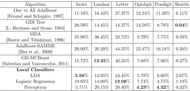
3.1 Multiclass performance of local linear classification. . . 64
3.2 Multiclass dataset properties used for L3M experiments. . . 66
3.3 L3M performance on multiclass data. . . 67
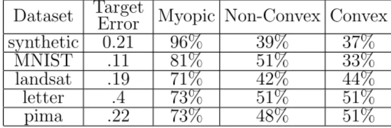
4.1 Performance comparison between the myopic budget classifier, non-convex budget cascade, and LP budget cascade. . . 105
1·1 Comparison of nearest neighbor graph and KLRR graph. . . 3
1·2 Example of budgeted classification cascade system. . . 8
2·1 Example of dense and sparse KLRR graphs. . . 24
2·2 Simulated line and circle data with KLRR clustering performance. . . 27
2·3 Simulated clusters data with anomaly detection performance . . . 30
2·4 Simulated linear data with anomaly detection performance. . . 31
2·5 KLRR anomaly detection performance on real data. . . 33
3·1 Local linear classifier structure and banana data example. . . 38
3·2 Local LDA performance on XOR. . . 46
3·3 Example of local classification symmetry. . . 47
3·4 L3M architecture and synthetic example. . . 52
3·5 L3M structure for multiple regions and decision boundaries on syn-thetic data. . . 55
3·6 Local linear classification online training performance. . . 61
3·7 Online local linear classification partitioning boundaries. . . 62
3·8 Historgram of classes in each region of a local perceptron. . . 63
3·9 Local linear classification performance vs. noise on real data. . . 65
3·10 L3M test error vs test computations on real data. . . 68
4·1 Example of converting general tree to binary tree. . . 82
4·2 Example of depth two budgeted learning system. . . 85
4·4 Synthetic data and performance of LP budget cascade. . . 104 4·5 Description of experimental data and performance of LP budget cascade.106 4·6 Synthetic data and performance of LP budget tree. . . 110 4·7 Performance of LP budget tree on landsat and image segmentation data.111 4·8 Comparison of system structure of LP budget tree and DAGGER. . . 113 4·9 Comparison of LP tree and budget DAG. . . 115
5·1 Adaptive privacy performance on Jester data. . . 126
-DP . . . -Differential Privacy
-NN . . . -Nearest Neighbors DAG . . . Directed Acyclic Graph DAGGER . . . Dataset Aggregation
ERM . . . Empirical Risk Minimization GDI . . . Gini Diversity Index
IID . . . Independent, Identically Distributed KLRR . . . Kernel Low-Rank Representation K-NN . . . K-Nearest Neighbors
L3M . . . Locally Linear Learning Machine LDA . . . Linear Discriminant Analysis
LLDA . . . Locally Linear Discriminant Analysis LLE . . . Locally Linear Embedding
LP . . . Linear Program
LRR . . . Low-Rank Representation MDA . . . Mixture Discriminant Analysis MDP . . . Markov Decision Process
PDF . . . Probability Distribution Function
POMDP . . . Partially Observed Markov Decision Process RBF . . . Radial Basis Function
ROC . . . Receiver Operating Characteristic SAMME . . . Stagewise Additive Modeling using a
Multi-class Exponential loss function SPC . . . Space Partitioning Classifier
SVD . . . Singular Value Decomposition SVM . . . Support Vector Machine UCI . . . University of California Irvine VC . . . VapnikChervonenkis
Chapter 1
Introduction
A common assumption in machine learning is the notion of local simplicity, that is, ex-amples which are near to each other have similar characteristics such as class labels or regression responses. Exploiting this assumption has many benefits in most learning tasks, as enforcing this not only potentially improves performance, but also can reduce the complexity of models or decision functions. Most often, the idea that neighboring examples have similar characteristics is enforced on globally complex models, where a complex function has the potential to fit or model every individual example but is penalized for complexity. For example, consider a universally consistent classifier such as a radial basis function (RBF) support vector machine (SVM). RBF classifiers have the flexibility to assign arbitrary labels to every unique data point, however in training the SVM, a regularization parameter penalizes overly complex decision boundaries, encouraging similar points to have be classified with the same labels.
Rather than constructing globally complex models and enforcing local examples to have similar behavior, we instead directly attempt to enforce this property through construction of systems that are locally simple yet globally complex. To this end, we address three main applications of this property of local similarity: modelling of high-dimensional structure as a union of simple structures, training piece-wise simple local learning functions such as local linear classifiers, and exploiting local similarity to reduce the cost of applying learning algorithms during test time.
non-linear low-rank manifold structure. Instead of learning a globally complex non-non-linear model, our goal is to learn a non-linear transformation that projects data onto linearly independent low-rank structures. In this projected space, examples lying on differ-ent structures are orthogonal, allowing for independdiffer-ent learning on each manifold. We present an efficient approach to finding these low-rank non-linear manifolds and prove that the proposed transformation projects data to a block-diagonal structure. Learning linear functions on this structure is equivalent to learning independent linear functions on each subspace, yielding an efficient algorithm for independent manifold learning.
Next, we examine the problem of exploiting simple local structure in loss-based learning. Under this assumption, we attempt to model learning functions using simple piece-wise functions composed of partitioning functions, which divide the space into multiple regions, and local learning functions which are applied independently in each partitioned region. First, we present a general framework to learn local functions under an empirical risk minimization (ERM) framework. By exploiting the structure of local loss functions, we show that learning the space partitioning of data can be reduced to a weighted supervised learning problem. This approach is applied to learn local classification and regression functions, with performance using extremely simple functions comparable to highly complex learning approaches while still maintaining computational tractability and generalization guarantees. For the case of supervised learning, we propose a globally convex approach to learning both the partitioning and classification functions based on a novel transformation of the empirical risk, allowing for efficient and repeatable minimization of the empirical risk.
We expand the local learning framework to the problem of adaptively acquiring sensor measurements during test time. In this setting, observing sensor measurements (features) during test time incurs a cost. Our goal is to learn a sensor acquisition
(a) Dense KNN Graph (b) Sparse KNN Graph
Figure 1·1: Left: K-nearest neighbor graph constructed on
densely-sampled 2-D simulated dataset. Right: K-nearest neighbor graph con-structed on sparsely-sampled 2-D simulated dataset.
system which adaptively acquires sensors for each example such that the cost of sensor measurements is minimized without loss of learning performance. We assume that neighboring examples are well characterized by similar sets of sensor measurements, and therefore adopt a strategy of partitioning the space into separate regions with only the necessary sensors acquired for each region.
1.1
Kernel Low-Rank Representations
The notion of distance, or more generally, similarity between observations, is at the root of most learning algorithms such as manifold learning, unsupervised clustering, semi-supervised learning, and anomaly detection. Most methods, at a basic level, are based on some function of Euclidean distance, such as the radial basis func-tions prevalent in supervised classification. Graph-based learning methods employ Euclidean distances to describe local neighborhoods for observations.
In many cases, notably sparsely sampled sets of data, Euclidean neighborhoods are not sufficient to represent underlying structure. Consider data drawn from two independent structures. Ideally, a graph would capture the structure of the data with
minimal connection between observations on separate structures. For densely sampled data on the manifolds, as shown in Fig. 1·1(a), local Euclidean neighborhoods tend to lie on the same independent manifold, and therefore the K-nearest neighbor graph using Euclidean distance captures the structure of the data. However, when the data is sparsely sampled, neighboring points in the Euclidean sense fail to lie on the same structure, as shown in Fig. 1·1(b).
For many datasets, observations are well described by either a single low-dimensional manifold or a union of multiple low-dimensional manifolds. Most methods deal with this scenario by patching together local neighborhoods or local linear subspaces. These local neighborhoods are generally based on local Euclidean balls around each data sample. Unfortunately, Euclidean distance does not capture low-dimensional structure of observations unless the manifold is highly sampled. In cases when ob-servations are sparsely sampled, are noisy, or lie in regions where the underlying manifold has high curvature, distance-based local approximations can be inaccurate and may fail to characterize the underlying manifold. Additionally, the notion of sim-ilarity based on Euclidean distance fails in the case of high-dimensional data. In these cases, the curse of dimensionality is only overcome based on the assumption that data lies on a lower-dimensional structure, in which case Euclidean distance in the high-dimensional space (and local neighborhoods in general) may be poor representations of similarity between observations.
We propose a novel approach to more accurately describe local neighborhoods by explicitly incorporating non-linear low-dimensional manifold structure of data.1 The
proposed approach yields a transformation which naturally partitions the data based on the underlying distinct manifolds upon which the data is embedded. Examples lying on distinct manifolds are transformed to representations with non-overlapping 1This chapter is based on work appearing in [Wang et al., 2011a, Wang et al., 2011b, Wang et al.,
support, implicitly partitioning the data and allowing for linear functions to be applied independently on each manifold by learning in this transformed space.
1.2
Local Loss-Based Learning
Next, we develop a novel approach to performing local empirical loss minimization by adaptively partitioning the feature space into different regions and learning inde-pendently in each region.2
We incorporate both feature space partitioning (reject classifiers) and region-specific functions into a single global empirical risk/loss function. We then optimize this global objective by means of coordinate descent, namely, by optimizing over one reject classifier or local function at a time. In this context we show that each step of the coordinate descent (learning a reject classifier) can be reformulated as a weighted supervised learning problem. This result is somewhat surprising in the context of partitioning and has broader implications. First, we can now solve feature space par-titioning through ERM and so powerful existing methods including boosting, decision trees and kernel methods can be used in conjunction for training flexible partitioning functions.
Second, because data is usually locally “well-behaved,” simpler local functions, such as linear classifiers, often suffice for controlling local risk. Furthermore, since complex boundaries for partitions can be approximated by piecewise linear functions, feature spaces can be partitioned to arbitrary degree of precision using linear bound-aries (reject classifiers). Thus the combination of piecewise linear partitions along with linear region classifiers has the ability to adapt to complex datasets leading to low training error. Yet we can prevent overfitting/overtraining by optimizing the number of linear partitions and linear region classifiers, since the VC dimension of 2This chapter includes work appearing in [Wang and Saligrama, 2012, Wang and Saligrama,
such a structure is reasonably small. In addition this also ensures significant robust-ness to label noise.
Limiting reject and region classifiers to linear methods has computational advan-tages as well. Since the datasets are locally well-behaved we can locally train with linear discriminant analysis (LDA), logistic regression and variants of perceptrons. These methods are computationally efficient in that they scale linearly with data size and data dimension. So we can train on large high-dimensional datasets with possible applications to online scenarios.
Our approach naturally applies to multi-class datasets. Indeed, we present some evidence that shows that the partitioning step can adaptively cluster the dataset into groups and letting region classifiers to operate on simpler problems. Additionally linear methods such as LDA, Logistic regression, and perceptron naturally extend to multi-class problems leading to computationally efficient and statistically meaningful results as evidenced on challenging datasets with performance improvements over state of the art techniques.
1.3
Adaptive Sensor Acquisition
We apply the same techniques developed for the local learning problem to the task of adaptive sensor acquisition.3 A majority of machine learning research has focused on improving performance of classification algorithms. Recently, costs in learning have gained importance, particularly the test time cost in decision making. This problem arises in classification systems constrained by a measurement acquisition budget. In this setting, a collection of sensor modalities with varying costs is available to the decision system. The objective is to learn a classifier that utilizes inexpensive sensing modalities for majority of decisions and requests the expensive (and more 3Portions of this chapter have been previously published in [Wang et al., 2014a, Wang et al.,
informative) sensors only for the few difficult decisions. Such a strategy maintains classifier accuracy while reducing the average acquisition cost per decision.
Several researchers [Chen et al., 2012, Trapeznikov et al., 2013, Trapeznikov and Saligrama, 2013, Xu et al., 2013] have made significant progress in developing algo-rithms to learn such decisions systems with promising experimental results. Due to the potentially high dimensional nature of sensor data, a discriminative learning ap-proach is used to learn decision functions directly by minimizing an empirical risk objective over a training set. However, the optimization problems are inherently non-convex and most solutions resort to alternative minimization schemes [Chen et al., 2012, Trapeznikov et al., 2013, Trapeznikov and Saligrama, 2013, Xu et al., 2013]. While experimental results demonstrate good performance, lack of global optimality prevents theoretical guarantees for the algorithms and the solutions.
In this work, we focus on the sequential decision framework studied in [Trapeznikov and Saligrama, 2013]. In this setting, the order in which sensors are acquired is given.4 Typically, earlier stages use cheap or fast sensors while later stages can acquire expen-sive or slow sensors. The decision function at each stage controls whether to stop and classify if enough information has been acquired for a confident decision or to continue and acquire the next sensor measurement (see Fig. 1·2). The authors in [Trapeznikov et al., 2013] introduce a global ERM problem and present an alternative minimization scheme to learn a decision function at each stage of the system.
Our main contribution is a novel convex formulation of the empirical risk prob-lem. We reformulate the empirical risk in [Trapeznikov and Saligrama, 2013] into maximization of sums of indicator functions. This key transformation enables us to introduce convex surrogates for the indicator functions and, in turn, results in 4For instance, such sequential decision problems arise in security screening and medical
applica-tions. In these scenarios, the objective is use a low cost modality (fast x-ray scanner, cheap blood test, etc) to make most classifications, and utilize an expensive modality (slow human inspection, invasive surgery) for as few as possible.
a convex optimization problem. Without our transformation, direct substitution of surrogates in the original empirical risk results in a non-convex bilinear formulation which is known to be NP-complete [Megiddo, 1988]. We upper-bound this reformu-lated objective and reduce it to a linear program (LP). This LP formulation learns sequential decision systems on real data and has the following advantages of convex programming: +1 +1 +1 -1 -1 -1 0 0 x= . . . . . . .. . . . . f1( x1 . . . .. . . . . ) f2( x1 x2 .. . . . . ) fk( x1 x2 .. . xk ) highest resolution lowest resolution increasing resolution Sample
Figure 1·2: Multi-Stage System consists of K stages. Each stage is a classifier with a reject option. The system incurs a penalty ofck atkth
stage if it rejects to seek more measurements. The kth classifier only sees the first k sensing modalities in making a decision.
Convergence: The linear program is guaranteed to converge to a solution,
whereas the alternating optimization approach of [Trapeznikov and Saligrama, 2013] has no such guarantee.
Global Optimum: The linear program converges to a globally optimal point,
whereas the alternating optimization approaches of [Trapeznikov and Saligrama, 2013, Bennett and Mangasarian, 1993, Wang and Saligrama, 2012] at best can only guarantee convergence to a local minimum if the algorithm converges.
Repeatability: No random initialization is necessary, whereas previous approaches ( [Trapeznikov and Saligrama, 2013,Bennett and Mangasarian, 1993,Wang and Saligrama, 2012]) for training sequential decisions all rely on multiple random initializations in an attempt to find a “good” local minimum.
Computational Efficiency: The linear program does not rely on random
ini-tialization or alternating optimization, allowing the solution to be found efficiently with a single optimization problem, whereas the alternating optimization approaches require repeatedly solving supervised learning problems. Additionally, given that the algorithm is a convex function, online training using approaches such as sub-gradient stochastic descent are feasible when the entire dataset is not available as a whole.
In the experimental section, we show that the proposed LP approach allows for dramatic reductions in average sensor acquisition cost while maintaining excellent classification performance on both synthetic and real world datasets. Additionally, we show performance that matches or exceeds non-convex optimization approaches while maintaining the previously mentioned advantages and clearly outperforming naive approaches.
We then further generalize to directed acyclic graph (DAG) structures with non-linear cost-structures. For structures where only a relatively small number of sensor subsets exist, we present a simple algorithm to train system decision functions. Along with added flexibility introduced by the new cost structure, we show that this simple algorithm is universally consistent and outperforms existing algorithms.
Finally, we extend the problem of learning under budgets to the structured predic-tion problem, where each example is composed of multiple elements, such as letters in a word. Finding policies over this structured space presents two major obstacles, the problem of learning a policy flexible enough to handle variable and possibly unseen structures (such as different length words) and to exploit the underlying structure of
the data in the policy. We show that the problem of learning a policy for budgeted structured prediction can be reduced to a weighted structured prediction problem, allowing for flexible policies to be efficiently trained using existing structured learning approaches.
1.4
Adaptive Privacy
An area of increasing interest is the protection of user privacy, in particular protection of private information of users. Recently, quantifying protection of privacy has been formalized by differential privacy [Dwork, 2006], however in machine learning tasks, this notion of differential privacy has generally been studied on a task-by-task basis. In the presence of multiple tasks, we attempt to construct a framework protecting the privacy of users while maximizing performance.
A fundamental trade-off in building learning systems under privacy constraints is the trade-off between learning performance and the privacy protection of the training dataset. Consider the problem of constructing a recommender system for movies. The goal is to learn a function for each new movie that, based on a subset of users who have viewed and rated the movie, will determine to whom the movie should be recommended. A fundamental trade-off in learning these functions is between performance and privacy of the raters. One approach to protecting the privacy of the raters is to apply a satisfactory level of differential privacy across all learned recommendation functions learned. Although this approach protects the privacy of the raters, it does so by assuming that each movie is best served by identical levels of privacy. This assumption fails to exploit that the performance vs. privacy trade-off is not identical across all movies, as some movies (such as popular blockbusters) have small performance gains from decreased levels of privacy, whereas other movies (such as documentaries on narrow subject-matter) have large performance gains from
decreased levels of privacy. Rather than apply a fixed level of privacy across all movies, we propose an adaptive privacy scheme that during assigns different privacy levels for each movie.
1.5
Organization
The dissertation is organized as follows:
Chapter 2 will describe our approach to learning low-rank non-linear structure. We formulate the non-linear low-rank problem, show that a robust closed-form so-lution exists, formulate a manifold anomaly detection algorithm, and demonstrate performance on synthetic and real-world data.
Chapter 3 presents an approach to training local learning functions under an ERM framework. After motivating the approach and presenting related work, we derive an alternating minimization framework. Next, we show an empirical risk transformation that allows for partitioning and classification functions to be jointly learned using convex optimization techniques.
Chapter 4 deals with incorporation of test-time costs in learning. We first present a linear program to incorporate test-time costs in classification. We extend test-time costs to other ERM problems and present preliminary work on including test-time costs in structured learning.
Chapter 2
Kernel Low-Rank Representation
In this chapter we examine the notion of locality and similarity in high-dimensions. A key component in many machine learning algorithms such as clustering and graph construction is the notion of similarity between examples, with the assumption that an example has closely related behavior, response, label, etc. as similar examples. These algorithms generally apply the Euclidean distance as the basis of measuring similarity between examples, which in the case of densely sampled data (with respect to observed dimensionality) often accurately captures underlying relationships among data. However, Euclidean distance often fails to capture similarity between sparsely sampled examples. This effect in particular arises in high dimensions, where the observed dimensionality of the data is much higher than the intrinsic dimensionality of the data, and Euclidean distance can is susceptible to noise. A standard approach to overcoming this issue is through the use of dimensionality reduction techniques, which seek to project the data from the observed high-dimensional space to an underlying low-dimensional space. Unfortunately, most dimensionality reduction techniques fail to account for the fact that observations are often not drawn from a single low-dimensional space, but from one of many possible low-low-dimensional spaces. To account for this, we present a data transformation such that examples lying in distinct non-linear low-dimensional spaces are dissimilar.
We first develop this non-linear low-rank transformation for a fixed set of data and show that examples on separate low-dimensional structures have low similarity
even in the presence of noise. This transformation is then extended to apply to new test examples to allow generalization on new observations, leading to an approach to constructing kernels incorporating low-dimensional non-linear structure. Next, we apply this notion of structural similarity to the anomaly detection problem to incor-porate structure into p-value estimation. Finally, we show improvement of empirical performance for a wide range of learning tasks by incorporating structural similarity.
2.1
Related Work
The most common notion of similarity is Euclidean distance, or a function of Eu-clidean distance such as radial basis functions. Graph-based learning methods em-ploy Euclidean distances to describe local neighborhoods for observations. K-nearest neighbors and -neighborhoods based on Euclidean distances are used in manifold learning (Isomap [Tenenbaum et al., 2000] and LLE [Roweis and Saul, 2000]), spec-tral clustering [Ng et al., 2001], anomaly detection algorithms [Zhao and Saligrama, 2009, Hero, 2007] and in label propagation algorithms for semi-supervised learn-ing [Zhu and Ghahramani, 2002].
The problem of determining an approximate representation for data using low-rank subspaces has recently drawn significant interest in the field of matrix comple-tion problems [Cand`es and Recht, 2009, Keshavan et al., 2009]. Methods for low-rank representations (LRR) of data drawn from multiple sources belonging to union of subspaces have also been developed [Liu et al., 2010, Wang et al., 2011a, Wang et al., 2011b]. Low-rank representations seek to segment data vectors such that each segmented collection belongs to a low-dimensional linear subspace. Low-rank representation of data is related to traditional simultaneous sparse representation techniques [Tropp et al., 2006] with important differences. The objective in simulta-neous sparsity is to decompose data vectors so that they have a common basis in a
dictionary. In both the rank-minimization and simultaneous sparsity problems, the goal is representation of data subject to a structural constraint. In comparison , we are not interested in exact representation of observations, but instead in embedding points in a linear plane, with the notion of low-rank structures as a means of defin-ing neighborhoods. In particular, our resultdefin-ing minimization resembles the problem posed by Liu et al. [Liu et al., 2010]. However, the problem posed in this paper can be solved in a computationally efficient manner, extended to nonlinear manifolds, and analyzed in the presence of noise.
2.2
Low-Rank Data Transformation
Consider a set of observations, X = [x1, x2, . . . xn], where xi ∈ Rd×1, approximately
embedded on multiple independent, low-dimensional manifolds. Our goal is to dis-cover these manifolds by using techniques to learn low-rank representations of the data. In the case where the observations are embedded on linear subspaces, the low-rank representation (LRR) problem [Liu et al., 2010] can be formulated as:
Z = min Z 1 2kX−XZk 2 F (2.1) s.t. Rank(Z) =R
wherek · kF is the Frobenius norm, and the solution, Z, is the minimum squared-error
linear embedding on a R-dimensional subspace. Relaxing the constraint in (2.1), the minimization can be equivalently written:
min Z 1 2kX−XZk 2 F +λ·Rank(Z) (2.2)
Optimizing the rank of a matrix is a non-convex, combinatorial optimization. The convex relaxation of rank, the nuclear norm, is substituted, resulting in the convex
optimization: min Z 1 2kX−XZk 2 F +λkZk∗ (2.3)
This related problem was originally posed as a subspace segmentation method by Liu et al. [Liu et al., 2010], who minimize the `2/`1 embedding error. A Kernelized
Low-Rank Representation (KLRR) formulation of the problem naturally follows for the case where data is embedded on nonlinear subspaces:
min Z 1 2kφ(X)−φ(X)Zk 2 F +λkZk∗ (2.4)
whereφ(·) is an expanded basis function with an associated kernel function,K(i, j) =
φ(i)Tφ(j). The form and parameters of the function φ(·) are an assumption on the
structure of the observations. Ideally, φ(·) is chosen such that all observations are well approximated in the expanded basis space with a linear low-dimensional ap-proximation while still maintaining the relationship between observations. As in all kernel methods, the accuracy of the approximation of the manifold is dependent on the ability of the kernel to fit the data. We refer only to the kernelized problem, as the linear problem is a specific case, whereφ(X) =X and K(X, X) =XTX.
Theorem 2.2.1. For λ≥0, the KLRR problem (2.4) is minimized by the
represen-tation:
Z∗ =U DλUT (2.5)
where the singular vectors, U, are found by the singular value decomposition (SVD) of the kernel matrix K(X, X) = φ(X)Tφ(X) = U DUT, and D
λ is the diagonal matrix defined Dλ(i, i) = 1− λ σi if σi > λ 0 otherwise (2.6)
and σi is the ith singular value of the kernel matrix.
Proof. The nuclear norm is unitarily invariant, so substituting ˆZ =UTZU, whereU
is the matrix of singular vectors of the kernel matrix produces an equivalent mini-mization UTZU = argmin ˆ Z 1 2kV DU T −V DZUˆ Tk2 F +λkZˆk∗ (2.7)
whereV DUT is the singular value decomposition of the matrixφ(X). The Frobenius norm is also unitarily invariant, and therefore pre-multiplying and post-multiplying the argument of the Frobenius norm by the matricesVT andU respectively produces the following minimization:
UTZU = argmin ˆ Z 1 2kD−D ˆ Zk2 F +λkZˆk∗ (2.8)
In the above minimization,Dis a diagonal matrix, resulting in ˆZalso being a diagonal matrix, as any off diagonal elements will increase the value of the cost function in both the Frobenius norm and nuclear norm terms. With a diagonal structure, the Frobenius norm is equivalent to the `2 norm of its weighted diagonal terms, and the
nuclear norm of ˜Z is equivalent to the `1 norm on its diagonal.
UTZU =Dλ = argmin ˆ Z 1 2kdiag D(I −Zˆ) k22 +λkdiag( ˆZ)k1 (2.9)
The solution to this minimization is given by the soft-thresholding operator, which gives the closed-form solution in the theorem statement.
The closed-form solution to the KLRR problem has previously been shown in [Wang et al., 2011b], with the closed-form solution to the linear low-rank representa-tion problem shown in [Favaro et al., 2011].
From Theorem 2.2.1, low-rank representations of high-dimensional expanded basis space observations can be computed efficiently using only kernel functions. Addition-ally, this solution has near block-diagonal structure for sets of observations existing
on independent subspaces1 in the expanded basis space.
Theorem 2.2.2. Given observations lying on independent subspaces in the expanded
basis space, the low-rank representation is near block-diagonal, with elements off-block-diagonal bounded: |zij| ≤λ v u u t X i:σi>λ 1 σi 2 (2.10)
where xi and xj lie on independent manifolds.
Proof. Consider the case of φ(X) = [φ(X1) φ(X2)], where φ(X1) ∈ RD×n1 and φ(X2) ∈ RD×n2 span independent subspaces and have rank r1 and r2, r1+r2 < D
and Rank(φ(X)) =r1+r2.
φ(X) is composed of observations lying on independent subspaces and therefore any point in φ(X1) orφ(X2) can be expressed as a linear combination of other points
in the setsφ(X1) orφ(X2), respectively. Given the compact SVD, φ(X) =UXΣXVXT,
which is equivalent to the full SVD with the singular vectors associated with zero singular values are removed in the basis UX and VX and the columns and rows
as-sociated with zero singular values removed from the singular value matrix SX. The
linear transformation
W = Σ−X1UXTφ(X) =VXT (2.11)
preserves the dependence structure of φ(X), resulting in the decomposition:
W = [B1 B2] hα 1 0 0 α2 i (2.12)
where B1 ∈ Rr1+r2×r1 and B2 ∈ Rr1+r2×r2 are basis matrices and α1 ∈ Rr1×n1 and α2 ∈Rr2×n2 are the representation associated with each independent subspace.
Sub-stituting the singular value decompositions α1 =U1Σ1V1T and α2 =U2Σ2V2T, W can
be expressed: W =B0 VT 1 0 0 VT 2 (2.13)
1Independent subspaces are defined as in [Liu et al., 2010], such that a set of subspaces are
where B0 = [B1U1Σ1 B2U2Σ2]. The matrix W is a set of singular vectors, so the
following property must hold:
W WT =B0 VT 1 0 0 V2T hV 1 0 0 V2 i B0T =B0B0T =I (2.14)
Therefore,B0 is an orthonormal matrix.
The solution to the KLRR problem can be expressed
Z∗ =VX(I−λΣ−X1)V T X =VXVXT −VXλΣ−X1V T X =hV01 V0 2 i B0TB0 V1T 0 0 VT 2 −VXλΣ−X1V T X (2.15)
The term VXVXT is block diagonal, so the inner product between representations
lying on separate independent subspaces can be bounded by examining the off-block-diagonal elements introduced by the term VXλΣ−X1V
T
X. This expression can
be bounded: kVXλΣ−X1V T Xk∞≤ kVXλΣ−X1V T XkF =λkΣ−X1kF (2.16)
From this structure, we construct measures of similarity that result in large dis-tance between observations on separate manifolds independent of Euclidean disdis-tance, resulting in separation of independent manifolds.
For reliable performance, the near block-diagonal structure of the KLRR matrix should remain in the presence of small perturbations. To demonstrate the robustness to noise, we bound the Frobenius norm of the off-diagonal elements when the kernel matrix is perturbed, guaranteeing near block-diagonal structure in the presence of noise.
Theorem 2.2.3. Consider a perturbed kernel matrix
e
K(X, X) =K(X, X) +E (2.17)
KLRR, Ze, is found using the matrix Ke(X, X). Define the matrix N to be the off diagonal blocks of the matrix Ze, such that for all zij ∈N, the observations xi andxj lie on independent manifolds. Then the matrix N is bounded:
kNkF ≤
4√2kEkF
σr−σe
(2.18)
where σr is the rth largest singular value of K(X, X) and σe is the largest singular value of the matrix E.
Proof. The right eigenvectors for K(X, X) can be expressed as in (2.13), with the perturbed right eigenvectors expressed:
e VX = ˜B ˜ V1T p1 p2 V˜2T (2.19)
where ˜B is an orthogonal matrix constructed as with B0,
From (2.15), the solution to the KLRR problem in the case of added perturbation can then be written:
e Z = ˜ V1D1V˜1T +pT2D2p2 V˜1TD1p1 +pT2D2V˜2 pT1D1V˜1+ ˜V2TD2p2 V˜2D2V˜2T +pT1D1p1 (2.20)
where D1 and D2 are diagonal matrices whose elements are less than 1 (as defined
in (2.6)). By the triangle inequality, the norm on the off diagonal elements can be bounded: ˜ V1TD1p1+pT2D2V˜2 pT 1D1V˜1+ ˜V2TD2p2 F ≤ kV˜1Tp1+pT2V˜2kF +kpT1D1V˜1+ ˜V2TD2p2kF = 2kV˜1TD1p1+pT2D2V˜2kF (2.21)
The term L1 can be bounded by further use of the triangle inequality:
V˜1TD1p1 +pT2D2V˜2 F ≤V˜1Tp1+pT2V˜2 F ≤ kV˜1Tp1kF +kpT2V˜2kF =kp1kF +kp2kF (2.22)
and guang Sun, 1990], Thm V.4.1) ksin ΘkF ≤ p kRk2 F +kSk2F δ (2.23)
with R and S defined:
R=Ke(X, X)U −VΣ
S =Ke(X, X)TV −UΣ
whereK(X, X) = UΣV is the singular value decomposition of the kernel matrix and
δ is a value chosen such that:
δ ≤ |σr−σe|
This bound can be simplified:
ksin ΘkF ≤ √
2kEkF
σr−σe
(2.24)
By the definition of canonical angles (Definition I.5.3 [Stewart and guang Sun, 1990]), this can be rewritten
k√I−Γ2kF ≤
√
2kEkF
σr−σe
(2.25)
where Γ2 is a diagonal matrix, whose ith diagonal element,γi2, can be written
γi2 =hv1ioi,˜v1io˜ii2 (2.26)
where oi and ˜oi are truncated vectors from some unitary matrices O and ˜O,
respec-tively, and v1i and ˜v1i are theith column of the matrices V1 and ˜V1, respectively. By
the Cauchy-Schwarz Inequality, γi2 can be bounded:
Substituting for Γ produces the bound: v u u t r X i=1 1− h˜v1i,v˜1ii ≤ √ 2kEkF σr−σe (2.28)
Given that the matrix ˜Ur is unitary, the bound can be further reduced: v u u tXr i=1 h˜v1i,v˜1ii+hp1i, p1ii − hα˜i,α˜ii ≤ √ 2kEkF σr−σe
where p1i is the ith column of the matrix p1. Therefore, we can bound the norm of
the matrix p1 kp1kF ≤ √ 2kEkF σr−σe (2.29)
Following the same steps produces an identical bound for the term kp2kF, and
there-fore:
kp1kF +kp2kF ≤
2√2kEkF
σr−σe
(2.30)
The theorem bound follows directly from (2.22) and (2.30).
Theorem 2.2.3 illustrates the robustness to noise of the low-rank representation. This is an adversarial bound, with the no restrictions placed on the structure of the perturbations. Given small perturbations such that σe ∈ o(σr), the norm of the
off diagonal elements can be bounded linearly with the norm of the perturbation. Therefore, small perturbations in the observations have small effects on the structure of the KLRR representation.
2.3
Transformation for Test Observations
Consider a new observation, xtest ∈ Rd×1. In order to represent the new
Equation (2.4). We project the data onto the expanded basis span of the KLRR representation, φ(X)Z, where Z is the KLRR on the training set X. The minimum norm projection can be calculated as a function of kernel functions.
ztest=Z ZTK(X, X)Z
−1
ZTK(X, xtest) (2.31)
The representation, ztest, can be treated as a new sample from the low-rank feature
space. This representation may be a poor representation of the original observa-tion if it does not lie on the manifold. One measure of how well a new observaobserva-tion is characterized by a manifold is by projecting the new observation onto the low-dimensional manifold (2.31), then measuring the residual energy of the observation in the expanded basis space.
rtest =kφ(xtest)−φ(X)ztestk2 (2.32)
This residual can also be calculated using only kernel functions and provides an evaluation of how well the low-rank representation fits a new observation.
2.4
Structured Kernel Design for Supervised and
Unsuper-vised Learning
From the low-rank representation, we now present methods of constructing kernels. The low-rank transformation of the raw data offers possibilities for designing kernels that incorporate the underlying structure in the data.
In order to exploit this structure we consider some specific PSD kernels, which are basically the dot product, i.e.,
wij =
ziTzj kzikkzjk
(2.33)
and jth columns of Z, respectively. The value wij is the magnitude of the cosine
of the angle between the vectors zi and zj. Given the near block-diagonal structure
of the KLRR matrix, as shown in Theorem 2.2.2, observations lying on independent subspaces have a very small similarity.
One issue with this similarity function is that it is undefined if either zi or zj is
identically zero. Consequently, we can define wij = 0 if either zi orzj is zero. With
this convention it is possible to show that this similarity satisfies the properties of PSD, i.e.,
N X i,j=1
cicjK˜(zi, zj)≥0
for any vector [c1, . . . , cN]. This follows directly given the fact that the kernel is an
inner-product of a rescaled version of the matrixZ. The similarity proposed in (2.33) captures the structure of the observations, however, the scaling information is lost. In order to incorporate structural information while preserving spatial relationships in the observation space, we propose the PSD kernel:
sij =K(xi, xj) = hzi, zji kzik · kzjk e −kxi−xjk2 2σ2 (2.34)
Two observations only have a large similarity if the observations lie on the same man-ifold and have a small geometric distance. If xi and xj lie on independent manifolds,
from the structure of the KLRR matrix, the angle between the observations is small, and therefore the similarity, sij, is also small. Alternatively, if the observations lie on
the same low-dimensional manifold, but have a large geometric distance, the expo-nential term drives the similarity to a small value. This kernel is a PSD kernel as it is composed of the product of two PSD kernels.
Figs. 2·1(a) and 2·1(b) demonstrate the effect of using structural similarity as opposed to Euclidean distance on the same sets of data as presented in Fig. 1·1.
(a) Dense Graph (b) Sparse Graph
Figure 2·1: Left: Graph for densely sampled 2-D simulated dataset
constructed by connecting the K-nearest structurally similar neighbors as defined by (2.34). Right: Graph constructed by connecting the K-nearest structurally similar neighbors as defined by (2.34), which captures the structure of the data. The Euclidean K-nearest neighbor graph fails to capture the structure of the data, as shown in Fig. 1·1.
In the case of densely sampled manifolds, using both notions of similarity construct graphs that capture the underlying structure of the data, as shown in Fig. 2·1(a). However, when the data is sparsely sampled, the use of structural similarity allows the graph to accurately characterize the underlying structure of the data, as shown in Fig. 2·1(b).
From the definition of similarity posed in (2.34), a means of defining distance between observations follows:
d(xi, xj) = p
sii+sjj−2sij (2.35)
The metric (2.35) defines a new set of distances between observations combining both the structural similarity of the data as well as the Euclidean distance of the data. Two observations have a small distance if and only if the observations lie on the same low-dimensional manifold and have a small distance in the observations space.
2.5
Manifold Anomaly Detection
The goal of our anomaly detection scheme is to define points not based on distance to nominal points, but instead based on distance to a low-dimensional manifold on which the training (nominal) points are embedded. In K-NN and -NN approaches, the underlying manifold is modeled by dense sampling of data points, whereas our approach no longer requires dense sampling of data points, but instead structural assumptions on the data. For a set of nominal observations embedded on a manifold, we propose a method of anomaly detection based on p-value estimation [Zhao and Saligrama, 2009].
Given a set of nominal training observations, X, a kernelized low-rank represen-tation, Z, is found as described in Section 2.2. For a new test observation, xt, a
corresponding low-rank representation, zt, is found through the update method
de-scribed in Section 2.3. From these low-rank representations, the residual of the test observation is compared to the residuals of the labeled observations:
pt = 1 n n X i=1 1w¯te−rt>w¯ie−ri (2.36)
where ri is the residual of theith labeled observation, calculated as shown in (2.32),
and ¯wt and ¯wi are the average angles cosine similarities of the representations as
de-fined in (2.33). The test observation is declared anomalous if pt> α. The proposed
anomaly detection characterizes the nominal set by a nonlinear low-dimensional man-ifold and uses a measure of similarity to the manman-ifold to determine if test observations are anomalous.
We modify our algorithm to simplify analysis. Assuming that nis even, we divide the training set into two sets S1 and S2. We compute the KLRR as defined by (2.4)
as defined by (2.31). The p-value of the new observation is then estimated as follows: ˆ pt= 1 |S2| X i∈S2 1w¯te−rt>w¯ie−ri (2.37)
The distribution of ˆptapproaches a uniform distribution over the range [0,1] given
thatxtis nominal and drawn from the same distribution as the nominal observations,
X. This follows from the lemma given by Zhao et al. [Saligrama and Zhao, 2012]:
Lemma 2.5.1. Given a function G(x) has the nestedness property, that is, for any
t1 > t2 we have x:G(x)> t1 ⊂ x:G(x)> t2. Then Px∼fn(G(x)≥G(η)) is
uni-formly distributed in [0, 1] if η ∼fn.
From this lemma, we can directly show that the distribution of ˆpt converges to a
uniform distribution.
Theorem 2.5.2. For a nominal test point, xt, drawn from the same distribution as
the labeled observations, X, pˆt converges to a uniformly distributed random variable in the range [0,1].
Proof. This follows directly from Lemma 2.5.1, as the function G(xi) = ¯wie−ri has
the nested property.
The distribution of pt converges to a uniform asn → ∞, and therefore the
2.6
Experimental Results
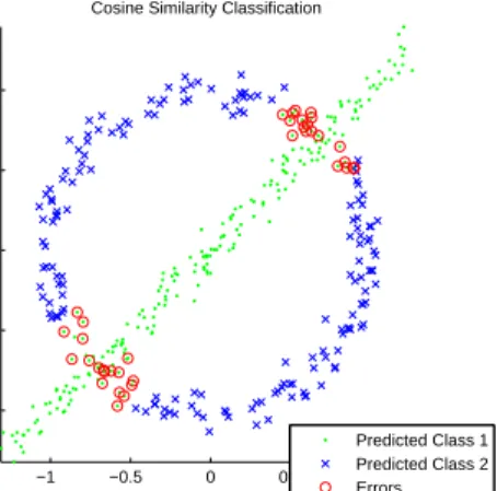
2.6.1 Clustering −1 −0.5 0 0.5 1 −1 −0.5 0 0.5 1Cosine Similarity Classification
Predicted Class 1 Predicted Class 2 Errors
Figure 2·2: 2-D simulated dataset. Two classes are constructed, a line and circle, with 200 observations in each class and random Gaussian noise added. Sample clustering results on simulated 2-D line-circle dataset are shown using k-means clustering on the structural similarity defined in Equation (2.33).
Dataset Classes Observation Kernel Similarity (W)
Simulated 2 49.4±0.1% 35.8±4.9% 9.4±0.1% Ionosphere 2 28.8±0.1% 28.9±0.1% 22.7±0% Iris 3 17.3±9.8% 15.3±8.5% 7.6±6.4% JAFFE 10 29.5±4.4% 25.5±5.0% 12.7±5.3%
Table 2.1: Average clustering error rates and standard deviation over 100 random initializations. Performance was compared for different representations: the original observations space (Observation), the ex-panded basis space (Kernel), and the cosine similarity space defined in (2.33) (Similarity (W)). For the JAFFE [Yang et al., 2010] and Iris databases [Eggermont et al., 2004], these performance rates are compa-rable to the best achieved results in literature and are achieved using an extremely simple algorithm (k-means clustering) on structured data.
To evaluate performance, k-means clustering [Hartigan and Wong, 1979] was per-formed on representations of the data, with the results shown in Table 2.1. The
k-means clustering algorithm was chosen as means to compare data representations due to its wide-spread use and lack of tuning parameters to be optimized. Initializa-tion was performed by assigning observaInitializa-tions to random clusters, with the error rates and standard deviations found for 100 random initializations. K-means clustering was tested on the data in the original feature space and in the kernel space. For the simulated data, the expanded basis was generated from a 3rd order inhomogeneous polynomial kernel multiplied with a Gaussian RBF kernel
K(xi, xj) = 1 +xTi xj 3 e (xi−xj)T(xi−xj) 2σ2
with the kernel parameterσ= 0.5. Note that this kernel does not perfectly transform the data to linear subspaces as the Gaussian RBF function does not map the two structures into linearly independent space. As a result, exact linear subspace recovery methods cannot be applied to this transform. For the Ionosphere, Iris, and JAFFE datasets, the expanded basis space was generated by Gaussian RBF kernel
K(xi, xj) =e
(xi−xj)T(xi−xj)
2σ2
with parameters σ= 1, σ= 2, and σ = 75, respectively.
Spectral clustering [Ng et al., 2001] performance using the previously described kernels is compared to similarity measures incorporating structure in Table 2.2. As with k-means clustering, inclusion of structure improved clustering performance in all example cases.
2.6.2 Anomaly Detection
We compare performance of our manifold anomaly detection approach with the K-nearest neighbors graph (K-NN) method presented by Zhao et al. [Zhao and Saligrama, 2009] and a One-Class SVM [Manevitz and Yousef, 2002]. We evaluate performance
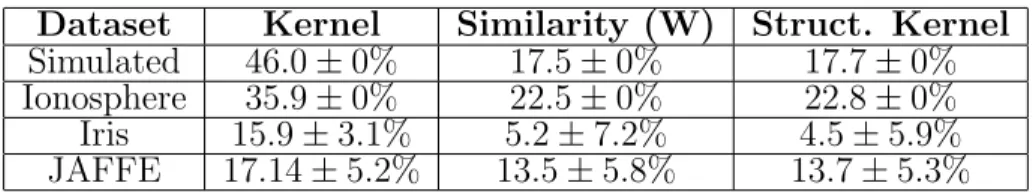
Dataset Kernel Similarity (W) Struct. Kernel
Simulated 46.0±0% 17.5±0% 17.7±0% Ionosphere 35.9±0% 22.5±0% 22.8±0% Iris 15.9±3.1% 5.2±7.2% 4.5±5.9% JAFFE 17.14±5.2% 13.5±5.8% 13.7±5.3%
Table 2.2: Average spectral clustering error rates and standard
de-viation over 100 random initializations. Performance was compared for different measures of similarity: the expanded basis space (Kernel), the cosine similarity space defined in (2.33) (Similarity (W)), and the structured kernel space defined in (2.34) (Structured Kernel). For the JAFFE [Yang et al., 2010] and Iris databases [Eggermont et al., 2004], these performance rates are comparable to the best achieved results in literature and are achieved using an extremely simple algorithm (k-means clustering) on structured data.
on simulated datasets, the Ionosphere dataset [Frank and Asuncion, 2010], the USPS Digits dataset [Hastie et al., 2003], and the JAFFE dataset [Lyons et al., 1998].
The simulated clusters dataset Fig. 2·3(a) consists of nominal data uniformly drawn from two Gaussian distributions with means [−2,0] and [2,0] and variances [0.02 0
0 0.02] and [00 0.3 0.3]. Anomalous data is uniformly drawn from either a uniform
distribution in the rectangle from [−3,−2] to [3,2] or a Gaussian distribution with mean [−2,0] and variance [0.3 0
0 0.3]. The motivation for this synthetic data is to present
an example where nearest neighbor distance alone may have difficulty separating anomalous points, as nominal examples are drawn from different Gaussians with drastically different variances.
The classifier was trained using 20 random nominal points, and performance was measured on a test set composed of 50 unobserved nominal points and 50 anomalous points, as shown in Fig. 2·3(a). A Gaussian radial basis function kernel (with σ = 0.5) was used to approximate the manifold, and performance was averaged over 100 randomly generated datasets, with average performance shown in Fig. 2·3(b).
−3 −2 −1 0 1 2 3 −1.5 −1 −0.5 0 0.5 1 1.5
Large and Small Clusters
Labeled nominal Unlabeled nominal Unlabeled anomalous
(a) Synthetic Clusters Data
0 0.1 0.2 0.3 0.4 0.5 0.6 0.7 0.8 0.9 1 0 0.1 0.2 0.3 0.4 0.5 0.6 0.7 0.8 0.9 1
False Positive Rate
True Positive Rate
Large/Small Clusters Dataset
K−LPE Method R−PE Method One Class SVM
(b) Clusters Performance
Figure 2·3: Left: Example of simulated clusters data. Training was
performed on 20 labeled nominal points (blue circles), and testing was performed on 50 unlabeled nominal points (green dots) and 50 unla-beled anomalous points (red crosses). Right: ROC curves averaged over 100 randomly generated datasets. Performance of p-value estima-tion using the KLRR residual is compared to p-value estimaestima-tion using a Euclidean neighborhood (2nd nearest neighbor) and One-Class SVM with µ= 0.5.
subspace [1,1], with nominal points having small random perturbations (drawn from a zero mean Gaussian distribution with variance [0.02 0
0 0.02]) and anomalous points having
large perturbations (drawn from a zero mean Gaussian distribution with variance [2 0
0 2]). As before, the classifer was trained using 20 random nominal points, and
performance was measured on a test set composed of 50 unobserved nominal points and 50 anomalous points, as shown in Fig. 2·4(a). The experiment was repeated using 100 randomly generated datasets, with an average performance shown in Fig. 2·4(b). A linear low-rank representation of the labeled points was used to approximate the manifold.
−10 −5 0 5 10 −8 −6 −4 −2 0 2 4 6 8 10
Sparse Linear Data
Labeled Nominal Points Unlabeled Nominal Points Unlabeled Anomolous Points
(a) Synthetic Linear Data
0 0.2 0.4 0.6 0.8 1 0 0.1 0.2 0.3 0.4 0.5 0.6 0.7 0.8 0.9 1
False Positive Rate
True Positive Rate
Sparse Linear Dataset
KLRR K−NN Method One Class SVM
(b) Linear Performance
Figure 2·4: Left: Example of simulated linear data. Training on 20
labeled nominal points (blue circles), testing on 50 unlabeled nominal points (green dots) and 50 unlabeled anomalous points (red crosses).
Right: ROC curves averaged over 100 randomly generated datasets.
Performance of p-value estimation using the KLRR residual is com-pared to p-value estimation using a Euclidean neighborhood (2nd near-est neighbor) and One-Class SVM with µ= 0.5.
labeled as nominal observations (drawn from the set which show evidence of structure in the ionosphere) and 30 observations were unlabeled for use as test data (uniformly drawn from both the observations showing evidence of structure like the nominal examples and examples showing no evidence of structure). A Gaussian radial basis function kernel was used (withσ = 1.5), and performance was compared to anomaly detection using a K-nearest neighbor graph and a One-Class SVM, as shown in Figure 2·5(a).
For the JAFFE dataset, 50 labeled nominal images were chosen from 3 random individuals (defined as nominal individuals) to construct the classifier. The test set was composed of 15 unobserved images randomly drawn from the nominal individuals and 100 anomalous images drawn from the other individuals. A Gaussian radial basis
function kernel (withσ= 75) was used to transform the data. The performance using the KLRR residual was compared to the use of a K-nearest neighbor graph for p-value estimation [Zhao and Saligrama, 2009] and a One-Class SVM [Manevitz and Yousef, 2002]. For the USPS Digits dataset, 200 nominal images (the digit 8) were labeled, with 167 unlabeled images randomly drawn from the unobserved nominal images and 33 anomalous images drawn from the other digits. A Gaussian RBF (with σ = 104)
was used to find the low-rank representation for both the USPS and JAFFE datasets, and the same kernel functions were used in the One-Class SVM. Performance was averaged over 100 randomly assigned datasets for all experiments, with performance shown in Fig. 2·5(b) and Fig. 2·5(c) for the JAFFE and USPS datasets, respectively. Use of the KLRR residual energy improved classification performance for simulated and real-world datasets. The ROC curves for the experiments lie above the ROC curves for either the K-nearest neighbor method or the One-Class SVM, indicating that the underlying nominal distribution likely lies on a low-dimensional manifold, and this low-dimensional structure is well approximated by the Z.
0 0.2 0.4 0.6 0.8 1 0 0.1 0.2 0.3 0.4 0.5 0.6 0.7 0.8 0.9 1
False Positive Rate
True Positive Rate
Ionosphere Dataset KLRR K−NN Method One Class SVM (a) Ionosphere 0 0.2 0.4 0.6 0.8 1 0 0.1 0.2 0.3 0.4 0.5 0.6 0.7 0.8 0.9 1
False Positive Rate
True Positive Rate
JAFFE Dataset KLRR K−NN One Class SVM (b) JAFFE 0 0.2 0.4 0.6 0.8 1 0 0.1 0.2 0.3 0.4 0.5 0.6 0.7 0.8 0.9 1
False Positive Rate
True Positive Rate
USPS Dataset
KLRR K−NN Method One Class SVM
(c) USPS
Figure 2·5: ROC curve on the Ionosphere, JAFFE, and USPS digits
dataset generated by averaging results over 100 random sets of labeled and unlabeled points. Performance using the KLRR residual and Eu-clidean distance (3rd, 3rd, and 9th nearest neighbor, respectively) for p-value estimation are shown, as is the performance of a One-Class SVM (µ= 0.5).
Chapter 3
Local Risk-Based Learning
In this chapter we examine approaches to constructing local classifiers, where we exploit the fact that learning functions, such as classification decision boundaries or regression functions, are often locally of low-complexity, though may not be globally well characterized by a single low-complexity function/model. Rather than learn a single high-complexity function to apply to the entire dataset, we instead attempt to partition the space into smaller regions, with simple functions applied within each region.
Our goal is to jointly learn functions which partition the feature space into sepa-rate regions and simple learning functions (such as classifier, regressors, rankers, etc.) applied to examples within each region. We first present an approach to learning local linear classifiers, where the data is partitioned by a cascade of linear functions into separate regions, with separate multiclass linear classification functions applied to each partitioned region. We show that under an alternating optimization frame-work, the problem of learning the partitioning functions is equivalent to solving a weighted binary classification problem and the problem of learning local classification functions simplifies to learning classification functions over subsets of the data. Next, we reformulate the empirical risk function for the local learning problem which yields a globally convex upper-bounding surrogate function, which allows for efficient global optimization as well as online training of classification and partitioning functions. We show that low-complexity local linear classification functions can efficiently yield
robust decision functions with performance comparable to high-complexity classifiers such as AdaBoost and Kernel SVM.
3.1
Related Work
Our approach fits within the general framework of combining simple classifiers for learning complex structures. Boosting algorithms [Freund and Schapire, 1997] learn complex decision boundaries characterized as a weighted linear combination of weak classifiers. In contrast our method takes unions and intersections of simpler decision regions to learn more complex decision boundaries. In this context our approach is closely related to decision trees [L. Breiman and Stone, 1984], and in particular de-cision trees with multivariate splits [Brodley and Utgoff, 1995]. One main difference is that decision trees typically attempt to greedily minimize some loss or a heuris-tic, such as region purity or entropy, at each split/partition of the feature space. In contrast our method attempts to minimize global classification loss. Also decision trees typically split/partition a single feature/component resulting in unions of rect-angularly shaped decision regions; in contrast we allow arbitrary partitions leading to complex decision regions.
Our work is loosely related to so called coding techniques that have been used in multi-class classification [Dietterich and Bakiri, 1995, Allwein et al., 2001]. In these methods a multiclass problem is decomposed into several binary problems using a code matrix and the predicted outcomes of these binary problems are fused to obtain multi-class labels. Jointly optimizing for the code matrix and binary classification is known to be NP hard [Crammer and Singer, 2000] and iterative techniques have been proposed [Guruswami and Sahai, 1999, Sun et al., 2005]. There is some evidence (see Sec. 3.4) that suggests that our space partitioning classifier groups/clusters multiple classes into different regions; nevertheless our formulation is different in that we do
not explicitly code classes into different regions and our method does not require fusion of intermediate outcomes.
Despite all these similarities, at a fundamental level, our work can also be thought of as a somewhat complementary method to existing supervised learning algorithms. This is because we show that space partitioning itself can be re-formulated as a supervised learning problem. Consequently, any existing method, including boosting and decision trees, could be used as a method of choice for learning space partitioning and region-specific decision functions.
We use simple linear classifiers for partitioning and region-classifiers in many of our experiments. Using piecewise combinations of simple functions to model a complex global boundary is a well studied problem. Mixture Discriminant Analysis (MDA) [Hastie and Tibshirani, 1996] models each class as a mixture of Gaussians, with linear discriminant analysis used to build classifiers between estimated Gaussian distributions. MDA relies upon the structure of the data, assuming that the true distribution is well approximated by a mixture of Gaussians. Local Linear Discrimi-nant Analysis (LLDA), proposed by Kim et al. [Kim and Kittler, 2005], clusters the data and performs linear discriminant analysis (LDA) within each cluster. Both of these approaches partition the data then attempt to classify locally. Partitioning of the data is independent of the performance of the local classifiers, and instead based upon the spatial structure of the data. In contrast, our proposed approach partitions the data based on the performance of classifiers in each region. A recently proposed alternative approach is to build a global classifier ignoring clusters of er-rors, and building separate classifiers in each error cluster region [Dekel and Shamir, 2012]. This proposed approach greedily approximates a piecewise linear classifier in this manner, however fails to take into account the performance of the classifiers in the error cluster regions. While piecewise linear techniques have been proposed in the
past [Dai et al., 2006,Toussaint and Vijayakumar, 2005], we are unaware of techniques that learn piecewise linear classifiers based on minimizing global ERM and allows any discriminative approach to be used for partitioning and local classification, and also extends to multiclass learning problems.
The optimization problem generated by the local linear learning problem has been previously studied in the context of bilinear separation [Bennett and Mangasarian, 1993]. In the bilinear separation problem, an attempt is made to directly minimize empirical risk. The empirical loss is expressed as a product of indicators which are approximated with hinge loss surrogate functions. This introduces a bilinear opti-mization problem whose globally optimal solution cannot be efficiently found. The space partitioning classifier framework can be seen as a generalization of the bilinear separation problem, where alternating minimization is used to train the partitioning and local classifiers, with each subproblem posed as a standard supervised learning problem. Space partitioning classifiers have been shown to have strong performance, however existing techniques can only guarantee convergence to a local minima without resorting to exhaustive search.
3.2
Learning Space Partitioning Functions
The goal in empirical risk minimization(ERM) is to learn a function,f(x), that maps features, x ∈ X, to an output, y ∈ Y, by minimizing a loss function, R(f), over training data (xi, yi), i= 1, 2, . . . , n: R(f) = 1 n n X i=1 L(xi, yi, f),
where L is the loss associated with the learning task, such as the indicator loss in supervised learning or the `2-loss in regression. Our goal is to minimize R(f) over
g1(x)
g2(x) Perceptron Logistic
Regression
AdaBoost Decision Tree
Figure 3·1: Left: Architecture of our system. Reject Classifiers,
gj(x), partition space and region classifiers, fj(x), are applied locally
within the partitioned region. Right: Comparison of our approach (upper panel) against Adaboost and Decision tree (lower panel) on the banana dataset [R¨atsch et al., 1998]. We use linear perceptrons and logistic regression for training partitioning classifier and region classi-fiers. Our scheme splits with 3 regions and does not overtrain unlike Adaboost.
of the family F dictates generalization of the learned function. If F is too simple, it often leads to large bias errors; if the f