Quantification-oriented learning based on reliable classifiers
Jose Barranquero, Jorge D´ıez, Juan Jos´e del Coz⇤
Artificial Intelligence Center (University of Oviedo), Campus de Viesques s/n, 33204, Spain
Abstract
Real-world applications demand effective methods to estimate the class distribution of a sample. In many domains, this is more productive than seeking individual predictions. At a first glance, the straightforward conclusion could be that this task, recently identified as quantification, is as simple as counting the predictions of a classifier. However, due to natural distribution changes occurring in real-world problems, this solution is unsatisfactory. Moreover, current quantification models based on classifiers present the drawback of being trained with loss functions aimed at classification rather than quantification. Other recent attempts to address this issue suffer certain limitations regarding reliability, measured in terms of classification abilities. This paper presents a learning method that optimizes an alternative metric that combines simultaneously quantifi-cation and classifiquantifi-cation performance. Our proposal offers a new framework that allows the construction of binary quantifiers that are able to accurately estimate the proportion of positives, based on models with reliable classification abilities.
Keywords: Quantification, Class distribution estimation, Performance metrics, Reliability, Multivariate predictions
1. Introduction
Any data scientist who had tackled real-world problems knows that there exist classifica-tion domains that are inherently complex, it being very difficult to obtain accurate predicclassifica-tions when focusing on each specific example; i.e., to achieve high classification accuracy. However, it is not so strange to require estimations about the characteristics of the overall sample instead,
⇤Corresponding author. J.J. del Coz ([email protected]). Phone/Fax: +34 985182501/985182125
Email addresses:[email protected](Jose Barranquero),[email protected](Jorge D´ıez),[email protected](Juan Jos´e del Coz)
mainly with respect to data distribution. Tentative application scopes include opinion mining [1], network-behavior analysis [2], remote sensing [3], quality control [4], word-sense disambigua-tion [5], monitoring of support-call logs [6], credit scoring [7] and adaptive fraud-detecdisambigua-tion [8], among others.
For instance, in order to measure the success of a new product, there is an increasing demand for methods for tracking overall consumer opinion, superseding classical approaches aimed at individual perceptions. To answer questions likehow many clients are satisfied with our new product?, we need effective algorithms focused on estimating the distribution of classes from a sample. This has emerging relevance when dealing with the tracking of trends over time [9], such as early detection of epidemics and endangered species, risk prevalence, market and ecosystem evolution, or any other kind of distribution change in general.
In many business, scientific and medical applications, it is sufficient, and sometimes even more relevant, to obtain estimations at an aggregated level in order to properly plan strategies. Companies could obtain greater returns on investment if they are able to accurately estimate the proportion ofeventsthat will involve higher costs or benefits. This will avoid wasting resources in guessing the class of each specific event; a task that usually reveals itself as complex, expensive and error-prone. For example, the estimation of the proportion of policy holders that will be involved in accidents during the next year, or the estimation of overall consumer satisfaction with respect to any specific product, service or brand.
In machine learning, the task of quantification isto accurately estimate the number of positive cases (or class distribution) in a test set, using a training set that may have a substantially different distribution[10]. Despite having many potential applications, this problem has barely been addressed within the community, and has yet to be properly standardized in terms of error measurement, experimental setup and methodology in general. Unfortunately, quantification has attracted little attention due to the mistaken belief of it being somewhat trivial. The key problem is that it is not as simple as classifying and counting the examples of each class, seeing as different distributions of train and test data can have a huge impact on the performance of state-of-the-art classifiers. The general assumption made by classification methods is that the samples are representative [11], which implies that the within-class probability densities,P r(x|y), and the a priori class distribution,P r(y), do not vary.
knowledge-based systems has been analyzed in several studies (see, for instance, [7, 12, 13]), suggesting that addressing distribution drifts is a complex and critical problem. Moreover, many papers focus on addressing distribution changes for classification, offering different views of what is subject to change and what is assumed to be constant. As in previous quantification-related papers, we focus only on studying changes in the a priori class distribution, while main-taining within-class probability densities constant. Domains of this kind are identified asY !X
problems by Fawcett and Flach [14]. Provided that we use stratified sampling [15], an example of situations whereP r(x|y)does not change is when the number of examples of one or both
classes is conditioned by the costs associated with obtaining and labeling them [16]. The explicit study of other types of distribution shifts, as well asX !Y domains, fall outside the scope of this paper (for further reading, we refer the reader to [17, 18, 19, 20]).
Receiver Operating Characteristic (ROC) analysis is quite a popular technique for the graphi-cal analysis of classification models [21]. A classifier may be trained for one particular operating condition, defined by one class distribution and cost proportion, but might then be deployed on a different condition. ROC curves visualize how the true positive rate (TPR) and the false positive rate (FPR) evolve for the same classifier for a range of thresholds. The threshold is the element to adapt a classifier to a given operating condition. ROC-based methods [8, 22] and cost curves [23] have been successfully applied to adjust the classification threshold, given that new class priors are known in advance. However, as already stated by Forman [10], these approaches are not use-ful for estimating class distributions from test sets. Similarly, if these new priors are unknown, two main approaches have been followed in the literature. On the one hand, most published papers focus on adapting the deployed models to the new conditions [24, 25, 26, 27, 28]. On the other hand, the alternative view is mainly concerned with enhancingrobustnessin order to learn models that are more resilient to changes in class distribution [29]. Whatever the case may be, the aim of these methods, although related, is quite different from that of quantification, as adapting a classifier for improving individual classification performance does not imply obtain-ing better quantification predictions, as we shall discuss later. Moreover, there exists a natural connection with imbalance-tolerant methods, mainly those based on preprocessing of data [30]. Actually, quantification was originally designed to deal with highly imbalanced datasets [10]; however, these preprocessing techniques are not directly applicable in changing environments.
binary-quantification model is based on standard classifiers, following a two-step training procedure. The first step is to train a classifier optimizing a classification metric, usually accuracy. The next step is then to study some relevant properties of this classifier. The aim of this second step is to correct the quantification prediction obtained from aggregating classifier estimates [10, 31].
An open question is whether it may be more effective to learn a classifier optimizing a quan-tification metric, instead of a classification performance measure. Conceptually, this alternative strategy is more formal, because the learning process takes into account the target performance measure. The main contribution of this paper is to explore this approach in detail.
The idea of optimizing a pure quantification metric during learning was introduced by Esuli and Sebastiani [1], although these authors neither implement nor evaluate it. Their proposal is based on learning a binary classifier with optimum quantification performance. We argue that this method has a pitfall. The key problem that arises when optimizing a pure quantification measure is that the resulting hypothesis space contains several global optimums. In practice, however, these optimum hypotheses are not equally good due to the fact that they differ in terms of the quality of their future quantification predictions. This paper claims that the robustness of a quantifier based on an underlying classifier is directly related to the reliability of such classifier. For instance, given several models showing equivalent quantification performance during train-ing, the learning method should prefer the best one in terms of its potential for generalization. As we shall analyze later, this factor is closely related with their classification abilities.
This lead us to further explore Esuli and Sebastiani’s approach with the aim of building a learning method able to induce more robust quantifiers based on classifiers that are as reliable as possible. In order to accomplish this goal, we introduce a new metric that combines both fac-tors. That is, a metric that combines classification performance with quantification performance, resulting in better quantification models.
As occurs with any other quantification metric, our proposal measures performance from an aggregated perspective, taking into account the whole sample. The difficulty involved in opti-mizing such functions is that they are not decomposable as a linear combination of the individual errors. Hence, not all binary learners are capable of optimizing them directly, requiring a more advanced learning machine. In this paper we adapt Joachim’s multivariate SVMs [32] to imple-ment our proposal and the idea presented by Esuli and Sebastiani. In order to validate these two approaches, another key contribution is to perform an exhaustive study in which we compare
them, along with several state-of-the-art quantifiers, by means of benchmark datasets from the UCI Machine Learning repository [33].
The paper is organized as follows. Section 2 introduces binary quantification as a learning task. Core concepts, notation and performance metrics for binary quantification are presented first. Then, a brief review of available quantification methods is provided, including those ap-proaches based on adjusted classification (Section 2.2.2) and threshold selection policies (Sec-tion 2.2.3). Quantifica(Sec-tion-oriented learning is analyzed in depth in Sec(Sec-tion 3. First, we describe the idea proposed by Esuli and Sebastiani. Then, we discuss a possible pitfall in their approach. Finally, we introduce our method (Section 3.3), based on a new quantification measure called
Q-measure. For a better understanding of our proposal, we describe Q-measure, both con-ceptually and graphically, in comparison with other performance measures. Section 4 reports the experiments performed, including the experimental setup, datasets, algorithms and statistical tests employed. The results are discussed in terms of different quantification measures. The paper ends by drawing some conclusions in Section 5.
2. Binary quantification
From a statistical point of view, the aim of a binary quantification task is to estimate the prevalence of an event or property within a sample. During the learning stage, we have a training set with examples labeled as positives or negatives; formally,D ={(xi, yi) : i = 1. . . S}, in whichxiis an object of the input spaceXandyi2Y={ 1,+1}. This dataset shows a specific distribution that can be summarized with the actual proportion of positives or prevalence. The learning goal is to obtain a model able to predict the prevalence (p) of another sample, usually
identified as the test set, that may show a markedly different distribution of classes. Thus, the input data is equivalent to that of traditional classification problems, but the focus is on the estimated prevalence (p0) of the sample, rather than on the class assigned to each individual
example. Notice that we usepandp0 to identify the actual and estimated prevalences of any
sample; these variables are not tied to training or test sets in any way.
Table 1 summarizes the notation that we shall employ throughout the paper. First, an algo-rithm is applied over the training set in order to learn a classifier. Then, we take the test set, whereP represents the count of actual positives andN the count of actual negatives. Once the
Table 1: Contingency table for binary problems
P N
P0 T P F P
N0 F N T N
(S=P+N=P0+N0)
individuals predicted as positives,N0the count of predicted negatives, whileT P,F N,T Nand
F P represent the count oftrue positives,false negatives,true negativesandfalse positives. We can then obtain the actual and estimated prevalences asp=P/Sandp0 =P0/S, respectively.
Notice again that these values can be computed for any set of examples, provided we use the classifier to predict their classes, even for the training set itself.
2.1. Performance measures for binary quantification
This section presents a brief review of several quantification loss functions that have been applied in previous quantification papers.
2.1.1. Estimation bias
According to Forman [10], the estimation bias is a natural error metric for quantification, which is computed as the estimated percentage of positives minus the actual percentage of posi-tives bias=p0 p=P 0 P S = F P F N S . (1)
When a method outputs moreF P thanF N, it shows a positive bias, and vice-versa. Thus, this
metric measures whether the model tends to overestimate or underestimate the proportion of the positive class. However, this metric is not useful for evaluating the overall performance in terms of average error (for a collection of sets), for the reason that negative and positive biases are neutralized. That is, as Forman points out,a method that guesses 5% too high or too low equally will often have zero biason average.
2.1.2. Absolute and squared errors
Forman proposed [10, 34, 35] theAbsolute Error(AE) between actual and predicted positive
prevalence as a standard loss function for quantification, that is simple, interpretable and directly applicable:
As an alternative toAE, Bella et al. [31] proposed theSquared Error(SE): SE= (p0 p)2= ✓P0 P S ◆2 = ✓F P F N S ◆2 . (3)
Actually,Mean Absolute Error(M AE) andMean Squared Error(M SE) are probably the most commonly used loss functions in regression problems. The concept of computing the ab-solute or squared error of real value estimations can be extended to any problem based on a continuos variable, likep. However, in the case of quantification, averaging among samples with different actual prevalence or from different domains has some implications that should be care-fully taken into account [10]. Note, for instance, that having a 5%AE for a test set with 45%
of positive examples may not be equivalent to obtaining the same error over a test set with only 10% of positive examples.
2.1.3. Kullback-Leibler Divergence
Kullback-Leibler Divergence (KLD), also known as normalized cross-entropy (see [1, 10]),
can be applied in the context of quantification. Assuming that we have only two classes, the final equation is: KLD = P S ·log ✓P P0 ◆ +N S ·log ✓N N0 ◆ . (4)
This metric determines the error made in estimating the predicted distribution (P0/S,N0/S)
with respect to the true distribution (P/S,N/S).
The main advantages ofKLDare that it may be more appropriate to average over different
test prevalences and more suitable for extending the quantification task for multiclass problems. However, a drawback ofKLDis that it is less interpretable than other measures, likeAE. More-over, we also need to define its output for those cases in whichP,N,P0 or N0 are zero (see
Section 3.4.2).
2.2. Quantification methods: state-of-the-art
The task of quantification has been formally addressed in a limited number of papers in recent years, with several complementary approaches having been proposed. Here we present a brief review of some of them.
2.2.1. Classify and count
The most simple method for building a quantifier is to learn a classifier, use the resulting model to label the instances of the sample and count the proportions of each class. This method is taken as a baseline by Forman [10], identifying it asClassify & Count(CC). Actually, it is straightforward to conclude that a perfect classifier would lead to a perfect quantifier. The key problem is that developing a perfect classifier is unrealistic, getting instead imperfect classifiers in real-world environments. This also implies that the quantifier will inherit the bias of the underlying classifier.
For instance, given a binary classification problem in which the learned classifier tends to misclassify some positive examples, then the derived quantifier will underestimate the propor-tion of the positive class. This effect becomes even more problematic in a changing environment, in which the test distribution is usually substantially different from that of the training set. Fol-lowing the previous example, when the proportion of the positive class goes up uniformly in the test set, then the number of misclassified positive instances increases and the quantifier will underestimate the positive class even more. Forman highlighted and studied this behavior for binary quantification, proposing several methods to tackle such bias.
2.2.2. Quantification via adjusted classification
With the aim of correcting classification bias, Forman [34] proposed a method termed Ad-justed Count(AC), in which the process is to train a classifier and estimate itstpr (true positive rate) andfpr(false positive rate) characteristics:
tpr =T P
P and fpr=
F P
N , (5)
through cross-validation over the training set. That is, for each fold we computeT P,F P,Pand Nto averagetpr andfpracross all folds. The next step is then to count the positive predictions
of the classifier over the test examples (i.e., just like the CC method) and adjust this value via the following formula
p00= p0 f pr
tpr f pr , (6)
wherep00denotes the adjusted proportion of positive test examples andp0 is the estimated
infeasible estimates ofp, requiring a final step in order to clip the estimation into the range[0,1]. Bearing in mind that the values oftpr andfpr are also estimates, we obtain an approxima-tion,p00, of the actual proportion,p. These two rates are crucial in understanding quantification
methods as proposed by Forman because they are designed under the assumption that the a priori class distribution,P r(y), changes, but the within-class probability densities,P r(x|y), do not.
This in turn ensures that both classifier characteristics,tprandfpr, are independent of changes
in class distribution (see [14]).
Note that due to (5), only thetprfraction of any shift inPwill be perceived by the
already-trained classifier (T P = tpr ·P). Moreover, the fpr fraction of N is misclassified as false positives (F P = fpr·N). In line with these observations, Forman [10] states the following theorem and its corresponding proof:
Theorem 2.1 (Forman’s Theorem). For an imperfect classifier, the CC method will underesti-mate the true proportion of positivespin a test set for p > p⇤, and overestimate forp < p⇤, wherep⇤ is the particular proportion at which the CC method estimates correctly; i.e., the CC
method estimates exactlyp⇤for a test set havingp⇤positives.
The overall conclusion is that a non-adjusted classifier tends to underestimate the prevalence of the positive class when it increases, and vice-versa.
2.2.3. Quantification via threshold selection policies
Given that the AC method allows any base classifier to be used to build a quantifier, the underlying learning process has attracted little attention. Much of the effort is once again due to Forman, who proposed a collection of methods based on training a linear SVM classifier, employing a posterior calibration of its threshold. The main difference between these methods is the threshold selection policy employed, aimed at alleviating some drawbacks of AC correcting formula from alternative perspectives.
A key problem related to the AC method is that its performance mainly depends on the degree of imbalance in the training set, worsening when the positive class is scarce [35]. In this case, the underlying classifier tends to minimize the false positive errors, which usually implies a low
tpr(see [22]) and a small denominator in Equation (6). This fact produces high vulnerability to
For highly imbalanced situations, the main intuition is that selecting a threshold that allows more true positives, even at the cost of many more false positives, could afford better quantifi-cation performance. The goal is to choose those thresholds where the estimates oftpr andfpr
have less variance or where the denominator in Equation (6) is large enough to be more resistant to estimation errors. For instance, theMaxmethod selects a threshold that maximizes the differ-ence betweentpr andfpr, while theXmethod chooses the threshold wherefprequals1 tpr,
avoiding the tails of both curves. In line with this last idea and assuming that positives constitute the minority class, the T50 method selects the threshold withtpr= 50%, avoiding only the tails
oftprcurve.
Notwithstanding, there is another problem related with all these methods arising from the fact that the estimation oftprandfprcan differ significantly from the real values. Forman thus proposed a more advanced method,Median Sweep(MS), based on estimating the prevalence for all thresholds during testing, in order to compute their median. This strategy is comparatively consistent, smoothing over estimation errors like in bootstrap-based algorithms and showing promising empirical results in practice.
2.2.4. Quantification via probability estimators
Bella et al. [31] have recently developed a family of methods they callprobability estimation & average. Their core proposal is to develop a probabilistic version of AC. First they introduce a simple method calledProbability Average(PA), which is clearly aligned with CC. The key dif-ference is that the classifier learned is probabilistic in this case. Once the probability predictions are obtained from the test dataset, the average of these probabilities is computed for the positive class as follows: p0= ˆ⇡P AT est( ) = 1 S S X i=1 P r(yi= +1|xi). (7)
As might be expected, when the proportion of positives changes between training and test, then PA will underestimate or overestimate as occurs with CC. These authors thus propose an enhanced version of this method, calledScaled Probability Average(SPA). Similar to CC and AC, the estimationp0 obtained from Equation (7) is corrected according to a simple scaling
formula:
p00= ˆ⇡SP A T est( ) =
p0 FPpa
whereTPpa andFPpa are values estimated from the training set, defined respectively asTP probability averageorpositive probability average of the positives
TPpa = ˆ⇡T rain ( ) = P
{i|yi=+1}P r(yi= +1|xi)
#{yi = +1}
,
andFP probability averageorpositive probability average of the negatives FPpa = ˆ⇡T rain ( ) =
P
{i|yi= 1}P r(yi= +1|xi)
#{yi= 1}
.
The expression defined in Equation (8) yields a probabilistic version of Forman’s adjustment defined in Equation (6). In their experiments, the SPA method outperforms CC, AC and T50; although they do not compare their proposal with other methods based on threshold selection policies like Max, X or MS.
3. Quantification-oriented learning
Esuli and Sebastiani [1] suggest the first training approach explicitly designed to learn a binary quantifier, in the context of a sentiment quantification task. However, a key limitation is that they neither implement nor validate it. This paper presents the first experiment results based on such an approach. Moreover, in this section we point out a possible pitfall in their idea and propose an alternative based on a new quantification measure, calledQ-measure.
3.1. Idea proposed by Esuli and Sebastiani
Although the training method that these authors describe is also based on building a clas-sifier, in this case the learning process optimizes the quantification error, without taking into consideration the classification performance of the model. Essentially, as their focus is on binary quantification problems, they argue that compensating the errors between both classes provides the means for obtaining better quantifiers. Therefore, the key idea is to optimize a metric derived from the expression|F P F N|. That is, a perfect quantifier should simply counterbalance all false positives with the same amount of false negative errors. In fact, all loss functions reviewed in Section 2.1 reach their optimum when this difference is equal to 0.
One difficulty in implementing this idea is that not all binary learners are capable of opti-mizing this kind of metric, because such functions are not decomposable as a linear combination
of the individual errors. Hence, this approach requires a more advanced learning machine, like
SV Mmulti[32], which provides an efficient base algorithm for optimizing non-linear functions computed from the contingency table (see Table 1). However, the straightforward benefit is that these methods address the quantification problem from an aggregated perspective, taking into account the performance over whole samples, which seems more appropriate for the problem in general.
Therefore, rather than learning a traditional classification model like
h:X !Y,
the core idea ofSV Mmulti is to transform the learning problem into one of multivariate pre-diction. That is, the goal is to induce a hypothesis,h¯, that maps all feature vectors of a sample ¯
x= (x1, . . . ,xS)to a tupley¯= (y1, . . . , yS)ofSlabels ¯
h: ¯X !Y¯,
in whichx¯2X¯ =XSandy¯2Y¯={ 1,+1}S. This multivariate mapping is implemented via a linear discriminant function
¯
hw(x) : arg max¯
¯
y02Y¯ {hw, (x,¯ y¯
0)i},
where¯hw(x)¯ yields the tupley¯0 = (y0
1, . . . , yS0)ofS predicted labels with a higher score ac-cording to the linear function defined by the parameter vector,w. The joint feature map, ,
describes the match between a tuple of inputs and a tuple of outputs. For the quantification-oriented methods presented in this paper, we use the same form proposed by Joachims for binary classification (x,¯ y¯0) = S X i=1 xiy0i.
This setup allows the learner to consider the predictions for all the examples and, in turn, optimize a sample-based loss function, . The optimization problem for obtainingwgiven a
non-negative is as follows min w,⇠ 0 1 2hw,wi+C⇠ (9) s.t. hw, (x,¯ y)¯ (x,¯ y¯0)i (¯y,y¯0) ⇠, 8y¯02Y \¯ y.¯
Notice that the constraint set of this optimization problem is extremely large, including one con-straint for each tupley¯0. Solving this problem directly is intractable due to the exponential size
ofY¯. Instead, we obtain an approximate solution applying Algorithm 1 described in [32]. The
key idea of this algorithm is to iteratively construct asufficient subsetof the set of constraints. In each iteration, the most violated constraint is added to the active subset of constraints. The search for this constraint depends on the target loss function. Given any metric computed from the con-tingency table, such as the quantification loss functions defined previously, Algorithm 2 [32] efficiently returns the most violated constraint. Note that the non-negativity condition imposed on implies that estimation bias cannot be optimized because it may return negative values.
3.2. Discussion
The two major frameworks described up to this point may present some drawbacks under specific conditions, as occurs with all learning paradigms. On the one hand, Forman’s methods provide estimations that are obtained in terms of modified classification models, optimized to improve their classification accuracy, instead of training them to reduce their quantification error. Although these algorithms showed promising quantification performance in practice, it seems more orthodox to build quantifiers by optimizing a quantification metric, as stated by Esuli and Sebastiani.
However, their proposal does not take classification accuracy into account as long as the quantifier balances the number of errors between both classes, even at the cost of obtaining a rather poor classifier. That is, Esuli and Sebastiani propose that the learning method should op-timize a quantification measure that simply deteriorates with|F P F N|. We strongly believe that it is also important for the learner to consider the classification performance as well. Our claim is that this aspect is crucial to ensure a minimum level of confidence for the deployed mod-els. The key issue is that pure quantification measures do not take into account the classification abilities of the model, producing several optimum points within the hypothesis search space (any that fulfillsF P =F N). However, some of these hypotheses are less reliable than others.
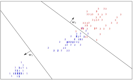
In order to analyze this issue we shall use the example in Figure 1, which represents all instances of the iris dataset. This training set contains three classes, with the same percentage for each of them. The learning task is to obtain a quantifier, not a classifier, for class 3 (i.e., class 3 is the positive class) while the negative class comprises classes 1 and 2 and we need a model to predict the prevalence of class 3. The figure depicts two hypotheses:w1andw2; the
former classifies all examples of class 1 as positives, while the latter predicts the majority of examples of class 3 as positives. Both hypotheses are perfect quantifiers for class 3 according to the training data. It is important to recall that all classes of the dataset have the same number of examples. For that reason, hypothesisw1is a perfect quantifier for class 3 because it predicts the
exact prevalence of class 1, which is the same prevalence as that of class 3. Any learning method that only takes quantification performance into account is not able to distinguish betweenw1
andw2. Our claim is thatw2should be prefered, because it is the better classifier, being more
robust to changes in class distribution. Actually,w1will quantify any change in the proportion
of class 3 in the opposite direction due to the fact that the hyperplane defined byw1is irrelevant
in the distinction between positive and negative examples. That is, usingw1, any increment in
the proportion of class 3 results in a decrement in the quantification of that class, and vice-versa. In contrast, the estimations ofw2increase or decrease in the same direction as these changes.
Interestingly enough, the strength of Forman’s approach is the weakness of the proposal presented by Esuli and Sebastiani, and vice-versa. While the latter approach emphasizes quan-tification ability during optimization, the former concentrates on building and characterizing classifiers in order to apply them as quantifiers. In this respect, our proposal may be able to soften these drawbacks, considering both classification and quantification performance during learning and thus producing more reliable and more robust quantifiers.
In fact, reliability is always a key issue when applying machine learning methods in practice. The question to be answered is how to measure the reliability that a quantifier offers, or whether it is reasonable for it not to be able to classify a minimum number of examples correctly.
The formal approach to obtain such quantifiers is to design a metric that somehow com-bines classification and quantification abilities and then apply a learning algorithm able to select a model that optimizes such a metric. This is the core idea of our proposal, which we shall introduce in the next section.
3 3 3 3 3 3 3 3 3 3 3 3 3 3 3 3 3 3 3 3 3 3 3 3 3 3 3 3 3 3 3 3 3 3 3 3 3 3 3 3 3 3 3 3 3 3 3 3 3 3 11 111 1 1 1 1 1 1 1 1 11 1 1 11 1 1 1 1 1 1 1 1 1 1 11 1 1 1 1 1 1 1 1 1 1 1 1 1 1 1 1 11 1 2 2 2 2 2 2 2 2 2 2 2 2 2 2 2 2 2 2 2 2 2 2 2 2 2 2 2 2 2 2 2 2 2 2 2 2 2 2 2 2 2 2 2 2 2 2 2 2 2 2 w2 w1
Figure 1: Graphical display of two conflicting perfect quantifiers
3.3. Our Proposal
Conceptually, the strategy of merging two complementary learning objectives is not new; we find the best example in information retrieval. The systems developed for such tasks are trained to balance two goals: retrieving as many relevant documents as possible, but discarding non-relevant ones. The metric that allows assessing how close these complementary goals are to being accomplished isF-measure[36]. Actually, this metric emerges from the combination of two ratios:recall(T P/P), which was already defined astprin (5), andprecision(T P/P0). In
a certain respect, we face a similar problem in quantification.
The first element of our proposal is a new family of score functions, inspired by the afore-mentionedF-measure. We need two core ingredients, a metric for quantification and another
for classification. The additional advantage of this approach is flexibility, in the sense that al-most any combination of measures can be potentially selected by practitioners. This new family is mainly aimed at guiding model selection during the learning stage. But, to a certain extent, it also allows the comparison of quantifiers trained with different approaches, whether or not they are based on these ideas. Evaluating quantifiers from this twofold perspective assists us in analyzing their reliability.
3.4. Q-measure: balancing quantification and classification
All the above leads us to present a new metric, calledQ-measure, which simultaneously
balances quantification and classification performance. The first point worth noting is that quan-tification is mostly explored for binary problems, in which the positive class is usually more relevant and must be correctly quantified. Thus, the design ofQ-measure described in this paper is focused on a binary quantification setting.
In summary, our approach is based on a similar concept to the standard classification metric
F-measure
F = (1 + 2)· 2precision·recall
·precision+recall , (10)
which balances an adjustable tradeoff betweenprecision andrecall. Analogously, we suggest
Q-measure, defined as
Q = (1 + 2)· 2cperf ·qperf
·cperf +qperf. (11)
The parameter allows weightingcperf andqperf measures, providing an AND-like behavior. Note thatcperf andqperf stand forclassification performanceandquantification performance, respectively. The selection of these metrics depends on the final learning goal, bearing in mind that they should be bounded between 0 and 1 in order to be effectively combined, representing the worst and best case, respectively.
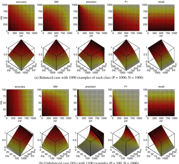
We now explore some alternatives through graphical representations. The motivation behind Figures 2, 3 and 4 is to enable us to analyze the behavior of different loss functions with respect to all combinations of values forF P andF N; both under balanced (2a, 3a and 4a) and unbalanced
(2b, 3b and 4b) training conditions. Each of the 2D plots is thexy-projection of its lower 3D
graph. Darker colors mean better scores. Notice also that 3D views are rotated over thez-axis in
order to make it easier to visualize the surfaces and that thex-axis ranges are different between balanced and unbalanced cases. Intuitively, a well-conceived learning procedure should tend to move towards those models whose scores fall within the darker areas. In other words, these graphs illustrate the hypothesis search space of each metric.
3.4.1. Classification performance
In Figure 2 we review some candidate classification metrics. In line with the binary quantifi-cation setting introduced previously, a natural choice forcperf isaccuracy, defined as(T P +
over an unbalanced binary problem, in which negatives are the majority class, resulting from a combination of several related classes (one-vs-all).
Other standard alternatives areF1, defined in Equation (10), and the geometric mean oftpr
(recall) andtnr (true negative rate), defined asGM =pT P/P·T N/N; i.e., the geometric
mean ofsensitivity andspecificity. GM is particularly useful when dealing with unbalanced
problems in order to mitigate the bias towards the majority class during learning [37].
An interesting property of bothtpr andtnr is that their respective search spaces are only
defined over one of the two classes, and hence they are invariant to changes in the dimension of the other. Notice that the graphical representation oftnr is equivalent to tpr or recall in Figure 2, though rotated 90o over thez-axis. That is whyGM also shows a constant shape between balanced (Figure 2a) and unbalanced cases (Figure 2b), with a proper scaling for the
y-axis. It is also worth noting thataccuracyapproachestnrwhen the size of the positive class is negligible ((T P +T N)/S⇡T N/N, whenP !0).
Therefore, we believe thataccuracymay be appropriate only in those cases in which we are
dealing with problems where both classes have a similar size, so we discard it. RegardingF1
andGM, although both could be appropriate, we finally focus onrecallfor our study. A
poten-tial benefit of maximizingrecall is that this may lead to a greater denominator in Equation (6),
providing more stable corrections. The fact that this metric is included inF-measureandGM
is also of interest, in order to weight the relevance of the positive class accordingly. Thus, this decision is also supported by the fact that the goal of the applications described in quantifica-tion literature focuses on estimating the prevalence of the positive class, which is usually more relevant.
In practical terms,Q-measureis able to discard pointlessqperf optimums thanks to the use
ofrecall. The key aspect is thatrecallacts as ahook, forcing the quantifier to avoid incoherent
classification predictions over the positive class. This reduces the amount ofF N errors,
conse-quently restricting the search space for the quantification part inQ-measure. Notice also that
pure quantification metrics tend to overlook positive class relevance in unbalanced scenarios.
3.4.2. Quantification performance
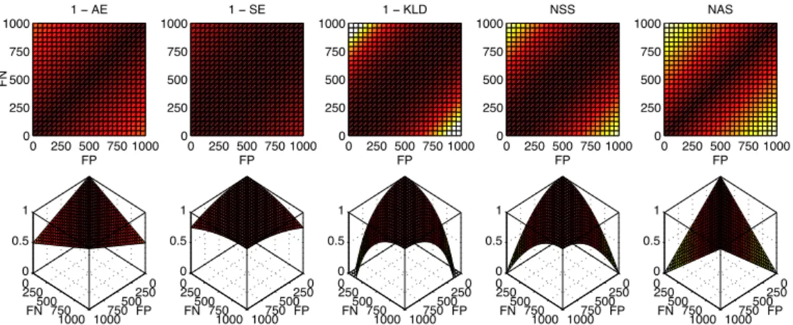
We considered several alternatives forqperf, starting from the standard measures described in Section 2. Unfortunately, none of the reviewed metrics fulfill all the requirements imposed by the design ofQ-measure. Hence, we also analyze the normalized versions ofAE andSE.
0 250 500 750 1000 0 250 500 750 1000 FP accuracy FN 0 250 500 750 1000 0 250 500 750 1000 0 0.5 1 FP FN 0 250 500 750 1000 0 250 500 750 1000 FP GM 0 250 500 750 1000 0 250 500 750 1000 0 0.5 1 FP FN 0 250 500 750 1000 0 250 500 750 1000 FP precision 0 250 500 750 1000 0 250 500 750 1000 0 0.5 1 FP FN 0 250 500 750 1000 0 250 500 750 1000 FP F1 0 250 500 750 1000 0 250 500 750 1000 0 0.5 1 FP FN 0 250 500 750 1000 0 250 500 750 1000 FP recall 0 250 500 750 1000 0 250 500 750 1000 0 0.5 1 FP FN
(a) Balanced case with 1000 examples of each class (P = 1000, N = 1000)
0 250 500 750 1000 0 25 50 75 100 FP accuracy FN 0 250 500 750 1000 0 25 50 75 100 0 0.5 1 FP FN 0 250 500 750 1000 0 25 50 75 100 FP GM 0 250 500 750 1000 0 25 50 75 100 0 0.5 1 FP FN 0 250 500 750 1000 0 25 50 75 100 FP precision 0 250 500 750 1000 0 25 50 75 100 0 0.5 1 FP FN 0 250 500 750 1000 0 25 50 75 100 FP F1 0 250 500 750 1000 0 25 50 75 100 0 0.5 1 FP FN 0 250 500 750 1000 0 25 50 75 100 FP recall 0 250 500 750 1000 0 25 50 75 100 0 0.5 1 FP FN
(b) Unbalanced case (9%) with 1100 examples (P = 100, N = 1000)
0 0.1 0.2 0.3 0.4 0.5 0.6 0.7 0.8 0.9 1
Figure 2: Graphical representation of all possible values for different classification loss functions, varyingF PandF N
between 0 and their maximum value, and with a fixed size for bothP andN(see inner captions). Darker colors mean better scores.
Figure 3 provides a graphical representation to assist in the interpretation and discussion of these functions. However, it is worth mentioning that the decision regardingqperf does not depend on whether we need to estimate the prevalence of one or both classes, because both values are complementary in binary problems (p= 1 n, wherenis the proportion of negatives orN/S).
Estimation bias is inappropriate because it can yield negative predictions. We also discard
KLDbecause it is not properly bounded and it yields unwieldy results when estimated
propor-tions are near 0% or 100%, like infinity or indeterminate values. According to [10], this problem can be resolved by backing off by half a count, which in our case means substituting the esti-mated proportion by|p0 0.5/S|, whenp02{0,1}. Moreover, as can be observed in Figure 3,
we also have to crop its range after subtracting from 1. These adjustments are not exempt from controversy, so we have focused on other alternatives.
We considerAE andSE, defined in Section 2.1.2, to be the most suitable candidates be-cause both are bounded between 0 and 1. However, they do not reach a value of 1 for almost any possible class proportion, except forp2{0,1}, moving further away from 1 in correlation
with the degree of imbalance (notice that theAE andSE values are substracted from 1 in
Fig-ure 3). This may result in an awkward behavior when combining these metrics withcperf in
Equation (11). Observe in Figure 2 that both components ofF-measurecover the whole range
between 0 (worst) and 1 (best case), and as required byQ-measure.
Looking at Equations (2) and (3) in more detail, we can see that, given a particular value for
p, their effective upper bounds aremax(p, n)andmax(p, n)2, respectively. Therefore we need
to normalize them. Moreover, as they are defined as loss functions, with the optimum at 0, we also need to redefine them as score functions. Taking into account these factors, we obtain two derived measures for quantification, denoted asNormalized Absolute Score(NAS)
NAS = 1 |p0 p| max(p, n) = 1
|F N F P|
max(P, N) , (12)
andNomalized Squared Score(NSS) NSS = 1 ✓ p0 p max(p, n) ◆2 = 1 ✓F N F P max(P, N) ◆2 . (13)
Figure 3 shows thatNAS andNSS are uniform and easily interpretable, presenting
0 250 500 750 1000 0 250 500 750 1000 1 − AE FP FN 0 250 500 750 1000 0 250 500 750 1000 0 0.5 1 FP FN 0 250 500 750 1000 0 250 500 750 1000 1 − SE FP 0 250 500 750 1000 0 250 500 750 1000 0 0.5 1 FP FN 0 250 500 750 1000 0 250 500 750 1000 1 − KLD FP 0 250 500 750 1000 0 250 500 750 1000 0 0.5 1 FP FN 0 250 500 750 1000 0 250 500 750 1000 NSS FP 0 250 500 750 1000 0 250 500 750 1000 0 0.5 1 FP FN 0 250 500 750 1000 0 250 500 750 1000 NAS FP 0 250 500 750 1000 0 250 500 750 1000 0 0.5 1 FP FN
(a) Balanced case with 1000 examples of each class (P = 1000, N = 1000)
0 250 500 750 1000 0 25 50 75 100 FP 1 − AE FN 0 250 500 750 1000 0 25 50 75 100 0 0.5 1 FP FN 0 250 500 750 1000 0 25 50 75 100 FP 1 − SE 0 250 500 750 1000 0 25 50 75 100 0 0.5 1 FP FN 0 250 500 750 1000 0 25 50 75 100 FP 1 − KLD 0 250 500 750 1000 0 25 50 75 100 0 0.5 1 FP FN 0 250 500 750 1000 0 25 50 75 100 FP NSS 0 250 500 750 1000 0 25 50 75 100 0 0.5 1 FP FN 0 250 500 750 1000 0 25 50 75 100 FP NAS 0 250 500 750 1000 0 25 50 75 100 0 0.5 1 FP FN
(b) Unbalanced case (9%) with 1100 examples (P = 100, N = 1000)
0 0.1 0.2 0.3 0.4 0.5 0.6 0.7 0.8 0.9 1
Figure 3: Graphical representation of all possible values for different quantification loss functions, varyingF PandF N
between 0 and their maximum value, and with a fixed size for bothP andN(see inner captions). Darker colors mean better scores.
quite similar to 1-KLD. From Figure 3a, we can see that when the problem is balanced, then all functions return the best scores on the diagonal. This represents where theF P andF N values neutralize each other, i.e., where|F P F N|cancels out. Figure 3b, on the other hand, provides
an example of an unbalanced problem. Once again, the optimal region lies above the line where these values cancel each other out, as may be expected.
For the sake of simplicity, we only focus onNASin our study. If we look for the maximum
possible value of|F P F N|, we conclude that it is always the number of individuals in the majority class. Assuming thatN is greater thanP, as is usual, the proof is that the worst
quan-tification score is obtained when all the examples of the minority class are classified correctly (T P =P andF N = 0), but all the examples of the majority class are misclassified (T N = 0
andF P =N), and thus Equation (12) evaluates to 0. With such a simple metric, we can see that the|F P F N|count is weighted in terms of the predominant class (denominator), forcing the output on the whole range between 0 and 1.
3.4.3. Graphical analysis ofQ-measure
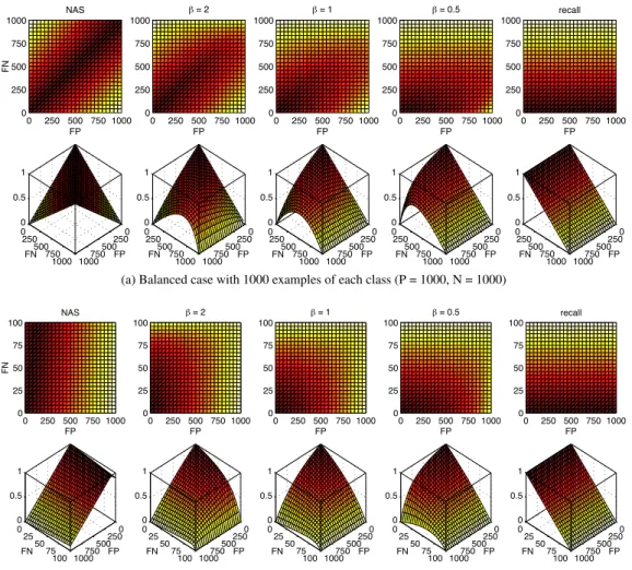
The graphical representation in Figure 4 provides an intuitive view to understand the behavior ofQ-measure, selectingrecallascperf andNASasqperf for Equation (11). Its interpretation
is exactly the same as in previous figures. Once again, we present two alternative learning con-ditions, balanced on the top (Figure 4a) and unbalanced on the bottom (Figure 4b). From left to right, we show different search spaces obtained from five target measures: firstNAS, then those obtained from three different values (Q2,Q1andQ0.5) , and finallyrecall. Notice thatrecall
andNAS are equivalent toQ0andQ1, respectively. When the value of is 1 (on the middle
graph), both the classification and quantification performance measures are equally weighted; when its value decreases to 0, thenQ-measure tends to be more similar tocperf; and when
it rises above 1, it tends to resembleqperf. Obviously, for the intermediate values of , the
obtained search spaces are significantly different from those of the seminal metrics.
In summary, recall drives the model to yield accurate predictions over the positive class,
minimizingF N. Whereas, on the other hand,NAS evaluates the compensation betweenF P
andF N. Hence, we have thatQ-measuredegrades when|F P F N|is high, but we are also penalizing those models with highF N.
Observing Figure 4, we can foresee that the search space defined by = 2will produce competitive quantifiers. An interesting property of this learning objective is thatQ2preserves
0 250 500 750 1000 0 250 500 750 1000 FP NAS FN 0 250 500 750 1000 0 250 500 750 1000 0 0.5 1 FP FN 0 250 500 750 1000 0 250 500 750 1000 FP β = 2 0 250 500 750 1000 0 250 500 750 1000 0 0.5 1 FP FN 0 250 500 750 1000 0 250 500 750 1000 FP β = 1 0 250 500 750 1000 0 250 500 750 1000 0 0.5 1 FP FN 0 250 500 750 1000 0 250 500 750 1000 FP β = 0.5 0 250 500 750 1000 0 250 500 750 1000 0 0.5 1 FP FN 0 250 500 750 1000 0 250 500 750 1000 FP recall 0 250 500 750 1000 0 250 500 750 1000 0 0.5 1 FP FN
(a) Balanced case with 1000 examples of each class (P = 1000, N = 1000)
0 250 500 750 1000 0 25 50 75 100 FP NAS FN 0 250 500 750 1000 0 25 50 75 100 0 0.5 1 FP FN 0 250 500 750 1000 0 25 50 75 100 FP β = 2 0 250 500 750 1000 0 25 50 75 100 0 0.5 1 FP FN 0 250 500 750 1000 0 25 50 75 100 FP β = 1 0 250 500 750 1000 0 25 50 75 100 0 0.5 1 FP FN 0 250 500 750 1000 0 25 50 75 100 FP β = 0.5 0 250 500 750 1000 0 25 50 75 100 0 0.5 1 FP FN 0 250 500 750 1000 0 25 50 75 100 FP recall 0 250 500 750 1000 0 25 50 75 100 0 0.5 1 FP FN
(b) Unbalanced case (9%) with 1100 examples (P = 100, N = 1000)
0 0.1 0.2 0.3 0.4 0.5 0.6 0.7 0.8 0.9 1
Figure 4: Graphical representation for the proposed loss functionQ-measure, varyingF P andF Nbetween 0 and their maximum value, and with a fixed size for bothPandN(see inner captions). Darker colors mean better scores. Each row shows the progression fromNAS( ! 1) torecall( = 0) through different values of .
the general shape of the optimal region defined byNAS, while degrading these optimums in consonance withrecall. That is, it offers the benefits of a quantification-oriented target, avoiding incoherent optimums (see Section 3.2).
We can also observe that, with = 1, we are forcing the learning method to obtain models
in the proximities of the lower values ofF P andF N. Specifically, in Figure 2b and Figure 4b,
we see that the shape ofQ1is reminiscent of that ofGM when the dataset is unbalanced. This
similarity arises from the fact that both sharerecall as one of their components, whileNASis
similar totnr on highly unbalanced datasets. In the extreme case, when the positive class is
minimal, the score1 AE is similar toNAS,accuracyandtnr
1 |F P F N| N+P ⇡1 F P N = T N N ⇡ (T P +T N) N+P , whenP !0.
Therefore, the main motivation for mixing inrecallis that using a pure quantification metric
could imply optimizing a similar target to that ofaccuracyortnr on highly unbalanced
prob-lems. In fact, as we shall analyze in the following section, the empirical results obtained from our experiments suggest that the behavior of a model learned thoughNAS is very similar to
that of CC, which is a classifier trained withaccuracy. In balanced cases, we believe that the
contribution ofrecall toQ-measurealso offers a more coherent learning objective, providing
more robust quantifiers in practice.
3.5. Learning algorithm
We use the same algorithms as described in Section 3.1 to implement a learning method for optimizingQ-measure. Actually, any metric obtained from the contingency table can be
optimized with these algorithms. This includes any variation ofQ-measurebased on different seminal metrics forcperf andqperf.
4. Experiments
The main objective of this section is to study the behavior of the quantification methods presented in this paper, comparing their performance with other state-of-the-art approaches. The main difference with respect to the first experimental designs followed for quantification is that our empirical analysis neither focuses on a particular domain, nor on a specific range of train or
test prevalences. We aim to cover a broader or more general scope, following the methodology that we have previously applied with success in [38]. Specifically, the experiments are designed to answer the following questions:
1. Do the empirical results support the use of a learner optimizing a quantification loss func-tion instead of a classificafunc-tion performance measure?
2. Do we obtain any clear benefit by considering both classification and quantification simul-taneously during learning?
The rest of the section is organized as follows. First we describe the experimental setup, including datasets, algorithms and statistical tests. We then present the results obtained from the experiments, evaluating them in terms ofAE andKLD. Finally, we discuss these results, with
the aim of providing answers to the aforementioned questions.
4.1. Experimental setup
As we introduced in [38], the required experiment methodology for quantification is rela-tively uncommon and has yet to be properly standardized and validated. The key difference with respect to traditional classification methodologies is that we need to evaluate performance over whole sets, rather than via individual classification outputs. Moreover, quantification as-sessment requires evaluating performance over a broad spectrum of test sets with different class distributions, instead of using a single test set.
We use benchmark datasets with known positive prevalences for performance measurement and comparison purposes, applying a variation of stratified 10-fold cross-validation. This setup preserves the original prevalence in all training iterations. Once a model has been trained with nine of the folds, the remaining one is used to generate 11 different random test sets with spe-cific positive proportions ranging from 0% to 100%, in steps of 10%, by means of stratified sampling [15]. This setup ensures that the within-class distributions,P r(x|y), are maintained
between training and test, as stated in Section 2.2.2, seeing that random resampling is uniform and stratified.
We presume that this variation in the testing conditions may be rather unnatural, requiring more appropriate data collections. Changes in training and test conditions should be extracted directly from different snapshots of the same population, showing natural shifts in their distri-bution. As yet, however, we have not been able to find suitable collections of publicly available
Table 2: Summary of datasets
Dataset Identifier Size Attrs. P os. N eg. %pos.
Balance Scale Weight & Distance (left) balance.1 625 4 288 337 46%
Balance Scale Weight & Distance (balanced) balance.2 625 4 49 576 8%
Balance Scale Weight & Distance (right) balance.3 625 4 288 337 46%
Contraceptive Method Choice (no use) cmc.1 1473 9 629 844 43%
Contraceptive Method Choice (long term) cmc.2 1473 9 333 1140 23%
Contraceptive Method Choice (short term) cmc.3 1473 9 511 962 35%
Cardiotocography Data Set (normal) ctg.1 2126 22 1655 471 78%
Cardiotocography Data Set (suspect) ctg.2 2126 22 295 1831 14%
Cardiotocography Data Set (pathologic) ctg.3 2126 22 176 1950 8%
Haberman’s Survival Data haberman 306 3 81 225 26%
Johns Hopkins University Ionosphere Database ionosphere 351 34 126 225 36%
Iris Plants Database (setosa) iris.1 150 4 50 100 33%
Iris Plants Database (versicolour) iris.2 150 4 50 100 33%
Iris Plants Database (virginica) iris.3 150 4 50 100 33%
Sonar, Mines vs. Rocks sonar 208 60 97 111 47%
SPECTF Heart Data spectf 267 44 55 212 21%
Tic-Tac-Toe Endgame Database tictactoe 958 9 332 626 35%
Blood Transfusion Service Center Data Set transfusion 748 4 178 570 24%
Wisconsin Diagnostic Breast Cancer wdbc 569 30 212 357 37%
Wine Recognition Data (1) wine.1 178 13 59 119 33%
Wine Recognition Data (2) wine.2 178 13 71 107 40%
Wine Recognition Data (3) wine.3 178 13 48 130 27%
datasets offering these specific features.
4.1.1. Datasets
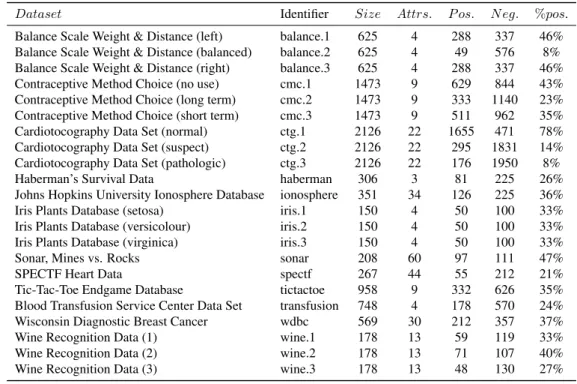
In order to enable a fair comparison between all methods, we select a collection of datasets from the UCI Machine Learning Repository [33], aiming to follow an unbiased criterion: prob-lems with ordinal or continuous features with, at the most, three classes and ranges from 150 to 2,500 examples. The summary of the 22 datasets fulfilling these constraints is presented in Table 2. As the percentage of positive examples ranges between 8% and 78%, this offers the possibility of evaluating the methods over significantly different training conditions. For datasets that originally have more than two classes, we follow a one-vs-all decomposition approach.
4.1.2. Algorithms
We take CC, AC, Max, X, T50 and MS as state-of-the-art quantifiers from Forman’s pro-posals, considering CC as the baseline. The underlying classifier for all these algorithms is a linear SVM from thelibsvmlibrary [39], with default parameters. The process of learning and threshold characterization, discussed in Sections 2.2.2 and 2.2.3, is common to all these models,
reducing the total time of the experiment and guaranteeing an equivalent root SVM for them all. Moreover, as Forman points out, the MS method may behave oddly when the denominator in Equation (6) is too small, making it advisable to discard any threshold withtpr fpr <1/4.
However, he does not make any recommendation in the case where there is no threshold that avoids said restriction. We therefore decided to fix these missing values with the values obtained by the Max method, which provides the threshold with the greatest value for that difference.
The group of models based on learning a classifier by optimizing a quantification metric consists of two approaches. On the one hand, there is our proposal, usingrecall andNAS as
seminal metrics (see Section 3.4). We consider threeQ-measurevariants: Q0.5, Q1 and Q2, representing models that optimize Equation (11) with at0.5,1 and2, respectively. On the other hand, we also include a method called NAS, which represents the approach suggested by Esuli and Sebastiani [1], usingNASas the target measure. The reason for choosingNASinstead of any other quantification loss function is that we believe that both approaches should use the same quantification metric, only differing in the fact that our proposal combines such metric with
recall. This guarantees a fair comparison. All these systems are learned by means ofSV Mmulti [32], described in Section 3.1.
4.1.3. Estimation oftpr andfpr
The estimations oftprandfprfor quantification correction, defined in Equation (6), are ob-tained through a standard 10-fold cross-validation after learning the root model. Other alterna-tives like 50-fold or LOO are discarded because they are much more computationally expensive and are prone to yield biased estimations, producing uneven corrections in practice.
It is also worth noting that we do not apply this correction for Q0.5, Q1, Q2 or NAS. Hence, their end models just count how many items are predicted as positive, like in the CC method. This decision is supported by the fact that our main objective is to evaluate the performance of models obtained from the optimization of these metrics, isolated from any other factor. Moreover, given that these systems are based onSV Mmulti, the estimation oftprandfpris much more expensive and it did not show a clear improvement in our preliminary experiments.
In fact, although the theory behind Equation (6) is well founded, in practice there exist cases where this correction involves a greater quantification error. However, these issues fall outside the scope of this study, offering an interesting opportunity to perform a more detailed analysis in
4.1.4. Adaptation of the Friedman-Nemenyi statistical test
Following Demˇsar [40], several two-step statistical test procedures were carried out. In each of these procedures, the first step consists of a Friedman test of the null hypothesis that all approaches perform equally in terms of a specific score or error metric. When this hypothesis is rejected, a Nemenyi post-hoc test is then conducted to compare the methods in a pairwise way. Both steps are based on the average of the ranks. The comparisons include 10 algorithms over 22 datasets or domains, evaluated over 11 different prevalences, resulting in 242 measurements per model.
Moreover, as Demˇsar notes, there are variations of the Friedman test which can consider multiple repetitions per dataset, provided that the observations are independent. However, since each collection of 11 test sets is sampled from the same fold, we cannot guarantee the assumption of independence among them. Thus, in order to take into account the differences between algo-rithms over several test prevalences from the same dataset, we first obtain their ranks for each test prevalence and then compute an average rank per dataset, which is used to rank algorithms on that domain. Therefore, we only consider the original number of datasets to calculate the crit-ical difference(CD), rather than using all test cases, resulting in a more conservative value. The reason for this is not only the fact that the assumption of independence is not fulfilled, but also that the number of test cases is not bound. Otherwise, simply taking a wider range of prevalences to test would imply a lower CD value, which appears to be unjustified from a statistical point of view and can be prone to distorted conclusions. Thus, we consider that the 10 algorithms are compared over 22 domains, regardless of the number of prevalences that are tested for each of them, resulting in a CD of 2.8883 for the Nemenyi test at the 5% significance level.
It should be stressed that we afford equal weight to all test prevalences. However, the method-ology that we propose is open to other interpretations, where the experimental design could assign larger weights to some prevalences or even the criterion followed to distribute the test prevalences may be neither linear nor uniform. This will depend mainly on the final aim of the experiment.
4.2. Results
This section presents the experimental results in terms of two standard quantification mea-sures:AE andKLD. Each of these measures provides a different perspective. In summary, we collect results from 22 datasets, applying a stratified 10-fold cross-validation for them all and
assessing the performance of the resulting model with 11 test sets generated from the remaining fold (see Section 4.1). Recall that only the quantification outputs provided by AC, X, Max, T50 and MS are adjusted by means of Equation (6).
4.2.1. Analysis ofAE measurements
The first approach that we follow is to represent the results for all test conditions in all datasets with a boxplot for each method under study. The idea is to show, in one single graph, the range of errors for a given metric of all the compared approaches. For instance, Figure 5a shows the ranges forAE measurements. Each box represents the first and third quartile by means of the lower and upper side, respectively, and the median or second quartile by means of the inner red line. The whiskers extend to the most extreme results not considered outliers, while outliers are plotted individually. In this case, we consider any point greater than the third quartile plus 1.5 times the inter-quartile range as an outlier. In this representation, it is better for a method to have lower quartile values, without outliers.
We distinguish three main groups in Figure 5a according to the learning procedure followed. The first one, including CC and AC, shows strong discrepancies between actual and estimated prevalences of up to 100%. These systems appear to be very unstable under specific circum-stances. The second group includes T50, MS, X and Max, all of which are based on threshold selection policies (see Section 2.2.3). The T50 method stands out as the worst approach in this group due to the upward shift of its box. The final group comprises theSV Mmulti models: Q0.5, Q1, Q2 and NAS. TheQ versions of this last group seems more stable than NAS, without extreme values over 70 and showing more compact boxes.
Friedman’s null hypothesis is rejected at the 5% significance level. The overall results of the Nemenyi test are shown in Figure 5b, in which each system is represented by a thin line, linked to its name on one side and its average rank on the other. The thick horizontal segments connect non significantly different methods at a confidence level of 5%. This plot suggests that Max and our proposal, represented by Q2, are the methods that perform best in this experiment in terms ofAEscore comparison for Nemenyi’s test. In this setting, we have no statistical evidence
of differences between the two approaches. Neither do they show clear differences with other systems. We can only appreciate that Max is significantly better than T50.
0 10 20 30 40 50 60 70 80 90 100 CC AC T50 MS X Max NAS Q2 Q1 Q0.5 0 10 20 30 40 50 60 70 80 90 100 CC AC T50 MS X Max NAS Q2 Q1 Q0.5
(a) Boxplots of all systems (b) Nemenyi at 5% (CD = 2.8883) Figure 5: Statistical comparisons in terms ofAEresults
10−3 10−2 10−1 100 101 CC AC T50 MS X Max NAS Q2 Q1 Q0.510 −3 10−2 10−1 100 101 CC AC T50 MS X Max NAS Q2 Q1 Q0.5
(a) Boxplots of all systems (b) Nemenyi at 5% (CD = 2.8883) Figure 6: Statistical comparisons in terms ofKLDresults
The mathematical proof is straightforward. Note that this is not fulfilled for other metrics, like
KLD.
4.2.2. Analysis ofKLD measurements
Although the analysis of AE results could be sufficient in most cases to discriminate an
appropriate model for a specific real-world task, we also provide a complementary analysis of our experiments in terms ofKLD. From Figure 5, we can see that the differences between some
systems are quite subtle in terms ofAE, while in Figure 6 we observe that these differences are
evidenced slightly more. For instance, Max and MS show larger outliers in terms ofKLD, due
to the fact thatKLDis similar to a quadratic error (see Figure 3).
Analyzing the results of the Nemenyi test in Figure 6b, our approach obtains the best rank, represented again by Q2, which is designed to give more weight to the quantification metric dur-ing learndur-ing. However, except for T50, this system is not significantly better than other models.
Q1, Max and NAS are also statistically differentiable from T50.
4.3. Discussion
In order to make the discussion of the results clearer, we now aim to answer the questions raised at the beginning of this section:
1. Do the empirical results support the use of a learner optimizing a quantification loss func-tion instead of a classificafunc-tion performance measure?
The fact is that the best ranks are dominated by these kinds of methods, in conjunction with Max. However, the differences with respect to other systems are not statistically significant in general.
In any case, our approach, initially suggested by Esuli and Sebastiani, is theoretically well-founded and is not based on any heuristic rule. From this point of view, we strongly believe that the methods presented here should be considered for future studies in the field of quantification. At the very least, they offer a different learning bias with respect to current approaches, which can produce better results in some domains.
Moreover, it should also be stressed that none of the quantification methods evaluated in this experiment are corrected by means of Equation (6), as discussed in Section 4.1.3. Thus, these methods may be considered variants of CC, which can be further improved with similar strategies to those applied in AC, Max, X, MS and T50.
2. Do we obtain any clear benefit by considering both classification and quantification simul-taneously during learning?
As we suspected, our variant obtains better results than the original proposal by Esuli and Sebastiani in terms of pure quantification performance (see AE results in Figure 5 and
KLDresults in Figure 6).
In some cases, NAS induces very poor classification models, despite benefiting from the definition of the optimization problem ofSV Mmulti, presented in Equation (9). Note
that the constraints on the optimization problem are established with respect to the actual class of each example ( (x,¯ y)¯ (x,¯ y¯0)), which would be produced by the perfect
classifier. Thus, the algorithm is biased to those models similar to the perfect classifier even when the target loss function is not. In practice, however, this learning bias is not able to overcome the drawbacks derived from the intrinsic design of pure quantification
metrics, which assigns an equal score to any model that simply neutralizes false positive errors with the same amount of false negative errors. Actually, our first intuition was that their proposal should provide even worse classifiers due to this fact. As we discuss in Section 3.2, the key problem is that pure quantification metrics produce several optimum points within the hypothesis search space, contrary to what occurs with other metrics, in which there is only one.
In summary, not only does our approach provides better quantification results than NAS, but we also consider it to be more reliable in general. Moreover, it is more flexible, al-lowing the practitioner to adjust the weight of both components ofQ-measuretaking into account the specific requirements of the problem under study by means of the parameter. In fact, provided that when ! 1our method optimizes only the quantification compo-nent, it includes NAS as a particular case. This calibration is not needed in general and can be fixed via the experimental design. As a rule of thumb, we suggest = 2, because, in
line with the discussion of Figure 4 and the analysis of the empirical results, it effectively combines the best features of both components.
5. Concluding remarks
Esuli and Sebastiani point out that state-of-the art quantification algorithms do not optimize the loss function applied during model selection or comparison. Following their line of research, we claim that optimizing only a quantification metric during model training does not sufficiently address the problem, as we could obtain quantifiers with poor quantification behavior due to an incoherent underlying model in terms of classification abilities. In this regard, the most important question behind our study is whether it is actually advisable to rely on quantification models that do not distinguish between positives and negatives at an individual level. But, how could this issue be mitigated during quantifier training? Formally, the way to solve any machine learning problem comprises two steps: define a suitable metric and design an algorithm that optimizes it. The combination ofQ-measureand the multivariate algorithm proposed by Joachims offers a
formal solution for quantifier learning.
Our main contributions are: i) the study of the first quantification-oriented learning approach, i.e., the first algorithm that optimizes a quantification metric; and ii) the definition of a parametric
loss function for quantification. This proposal is not only theoretically well-founded, but also of-fers competitive performance on benchmark datasets compared with state-of-the-art quantifiers.
Acknowledgments
This work was supported in part by the Spanish Ministerio de Econom´ıa y Competitividad, under research project TIN2011-23558. The contribution of Jose Barranquero was also sup-ported by FPI grant BES-2009-027102.
References
[1] A. Esuli, F. Sebastiani, Sentiment quantification, IEEE Intelligent Systems 25 (2010) 72–75.
[2] L. Tang, H. Gao, H. Liu, Network quantification despite biased labels, in: Proceedings of the 8th Workshop on Mining and Learning with Graphs, ACM, pp. 147–154.
[3] A. Guerrero-Curieses, R. Alaiz-Rodriguez, J. Cid-Sueiro, Cost-sensitive and modular land-cover classification based on posterior probability estimates, International Journal of Remote Sensing 30 (2009) 5877–5899. [4] L. S´anchez, V. Gonz´alez-Castro, E. Alegre-Guti´errez, R. Alaiz-Rodr´ıguez, Classification and quantification based
on image analysis for sperm samples with uncertain damaged/intact cell proportions, in: Image Analysis and Recognition, LNCS 5112, Springer, 2008, pp. 827–836.
[5] Y. Chan, H. Ng, Estimating class priors in domain adaptation for word sense disambiguation, in: Proc. of the 21st International Conference on Computational Linguistics, ACL, pp. 89–96.
[6] G. Forman, E. Kirshenbaum, J. Suermondt, Pragmatic text mining: minimizing human effort to quantify many issues in call logs, in: Proceedings of ACM SIGKDD’06, ACM, pp. 852–861.
[7] D. Hand, Classifier technology and the illusion of progress, Statistical Science 21 (2006) 1–14.
[8] F. Provost, T. Fawcett, Robust classification for imprecise environments, Machine Learning 42 (2001) 203–231. [9] T. Rakthanmanon, E. Keogh, S. Lonardi, S. Evans, MDL-based time series clustering, Knowledge and Information
Systems 33 (2012) 371–399.
[10] G. Forman, Quantifying counts and costs via classification, Data Mining and Knowledge Discovery 17 (2008) 164–206.
[11] R. O. Duda, P. E. Hart, D. G. Stork, Pattern Classification, John Wiley & Sons, 2001.
[12] M. Kelly, D. Hand, N. Adams, The impact of changing populations on classifier performance, in: Proceedings of ACM SIGKDD’99, pp. 367–371.
[13] R. Alaiz-Rodr´ıguez, N. Japkowicz, Assessing the impact of changing environments on classifier performance, in: Advances in AI, LNCS 5032, Springer-Verlag, 2008, pp. 13–24.
[14] T. Fawcett, P. Flach, A response to Webb and Ting’s on the application of ROC analysis to predict classification performance under varying class distributions, Machine Learning 58 (2005) 33–38.
[15] J. Fleiss, B. Levin, M. Paik, Statistical Methods for Rates and Proportions, Wiley Series in Probability and Statistics, John Wiley & Sons, 2003.