Real-time Traffic Flow Detection and Prediction Algorithm: Data-Driven Analyses on Spatio-Temporal Traffic Dynamics

(1)

University of Tennessee, Knoxville

Trace: Tennessee Research and Creative

Exchange

Doctoral Dissertations Graduate School

12-2017

Real-time Traffic Flow Detection and Prediction

Algorithm: Data-Driven Analyses on

Spatio-Temporal Traffic Dynamics

Bumjoon Bae

University of Tennessee, [email protected]

This Dissertation is brought to you for free and open access by the Graduate School at Trace: Tennessee Research and Creative Exchange. It has been accepted for inclusion in Doctoral Dissertations by an authorized administrator of Trace: Tennessee Research and Creative Exchange. For more information, please [email protected].

Recommended Citation

Bae, Bumjoon, "Real-time Traffic Flow Detection and Prediction Algorithm: Data-Driven Analyses on Spatio-Temporal Traffic Dynamics. " PhD diss., University of Tennessee, 2017.

(2)

To the Graduate Council:

I am submitting herewith a dissertation written by Bumjoon Bae entitled "Real-time Traffic Flow Detection and Prediction Algorithm: Data-Driven Analyses on Spatio-Temporal Traffic Dynamics." I have examined the final electronic copy of this dissertation for form and content and recommend that it be accepted in partial fulfillment of the requirements for the degree of Doctor of Philosophy, with a major in Civil Engineering.

Lee D. Han, Major Professor We have read this dissertation and recommend its acceptance:

Hamparsum Bozdogan, Christopher Cherry, Hyun Kim

Accepted for the Council: Carolyn R. Hodges Vice Provost and Dean of the Graduate School (Original signatures are on file with official student records.)

(3)

Real-time Traffic Flow Detection and Prediction Algorithm:

Data-Driven Analyses on Spatio-Temporal Traffic Dynamics

A Dissertation Presented for the

Doctor of Philosophy

Degree

The University of Tennessee, Knoxville

Bumjoon Bae

December 2017

(4)

(5)

iii

DEDICATION

To my wife and son, Lina Ryu and Jiho B. Bae, for all their endless love and

support.

(6)

iv

ACKNOWLEDGEMENTS

I would like to express my deep gratitude to my advisor, Dr. Lee D. Han for his support and guidance during my graduate studies. I was very fortunate to have him as my advisor who continually and convincingly conveyed keen insight with regard to my research. Without his encouragement, I would never finish my dissertation successfully. I would also like to thank my statistics advisor, Dr. Hamparsum Bozdogan, and my committee members, Dr. Christopher Cherry and Dr. Hyun Kim for serving on my committee, as well as Dr. Asad Khattak for

helping me improve my study.

I am truly grateful to Hyeonsup Lim for his endless support and excitement about research and life in Knoxville as my mentor. I will definitely miss the days in Knoxville with him.

Last, but not least, I would like to thank all my lab mates: Stephanie Hargrove, Jianjiang Yang, Yang Zhang, Yuandong Liu, Zhihua Zhang, Pankaj Dahal, Brandon Whetsel, Brandon Worley, Kwaku Boakye, Meng Zhang, Ziwen Ling, Jun Liu, Ranjit Khatri, Nirbesh Dhakal, Ali Boggs, Behram Wali, Xiaobing Li, Mohsen Kamrani, Nima Hoseinzadeh and many others.

(7)

v

ABSTRACT

Traffic flows over time and space. This spatio-temporal dependency of traffic flow should be considered and used to enhance the performance of real-time traffic detection and prediction capabilities. This characteristic has been widely studied and various applications have been developed and enhanced. During the last decade, great attention has been paid to the increases in the number of traffic data sources, the amount of data, and the data-driven analysis methods. There is still room to improve the traffic detection and prediction capabilities through

studies on the emerging resources. To this end, this dissertation presents a series of studies on real-time traffic operation for highway facilities focusing on detection and prediction.

First, a spatio-temporal traffic data imputation approach was studied to exploit multi-source data. Different types of kriging methods were evaluated to utilize the spatio-temporal characteristic of traffic data with respect to two factors, including missing patterns and use of secondary data. Second, a short-term traffic speed prediction algorithm was proposed that provides accurate prediction results and is scalable for a large road network analysis in real time. The

proposed algorithm consists of a data dimension reduction module and a

nonparametric multivariate time-series analysis module. Third, a real-time traffic queue detection algorithm was developed based on traffic fundamentals

combined with a statistical pattern recognition procedure. This algorithm was designed to detect dynamic queueing conditions in a spatio-temporal domain rather than detect a queue and congestion directly from traffic flow variables. The algorithm was evaluated by using various real congested traffic flow data. Lastly, gray areas in a decision-making process based on quantifiable measures were addressed to cope with uncertainties in modeling outputs. For intersection control type selection, the gray areas were identified and visualized.

(8)

vi

LIST OF TABLES

Table 1-1 Description of RTMS stations and corresponding HERE links. ... 12

Table 2-1 Temporal scale effects on 5-minute prediction performance using RTMS. ... 46

Table 2-2 Comparison of 5-minute prediction performance for RTMS. ... 50

Table 2-3 Prediction performance for multi-step predictions. ... 54

Table 2-4 Comparison of 5-minute prediction performance for NPMRDS. ... 56

Table 3-1 Empirical shock wave speeds and queue arrival time prediction errors. ... 86

(11)

ix

LIST OF FIGURES

Figure 1-1 Map of the selected RTMS stations on I-40 eastbound in Knoxville. . 11

Figure 1-2 Collected five-minute average speed points: (a) RTMS and (b) HERE. Each dot represents an observation point in spatiotemporal dimension. ... 14

Figure 1-3 Research design. ... 18

Figure 1-4 Scatter plots between RTMS and HERE: (a) original speed, and (b) log-transformed speed. ... 20

Figure 1-5 Missing scenario plots with 10% missing rate: (a) MCAR, (b) MAR, and (c) MNAR. Each dot represents observation point in spatiotemporal dimension. ... 22

Figure 1-6 Theoretical semivariograms: (a) OK, (b) OCK, and (c) SCK. ... 23

Figure 1-7 Imputed Speed using OK without missing values: (a) RTMS and (b) HERE. ... 25

Figure 1-8 MAE and MAPE comparisons. ... 27

Figure 2-1 Proposed speed prediction algorithm. ... 36

Figure 2-2 Data dimension rate of MSSA by using PCA. ... 40

Figure 2-3 Speed data visualizations: (a) RTMS – September 23, 2016; (b) RTMS – September 30, 2016; and (c) NPMRDS – February 3, 2017. ... 44

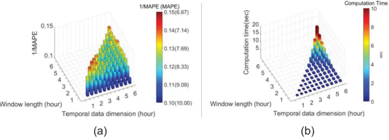
Figure 2-4 RTMS with different temporal dimension and window length (September 30, 2016): (a) MAPE and (b) computation time. ... 48

Figure 2-5 NPMRDS with different temporal dimension and window length: (a) MAPE and (b) computation time. ... 48

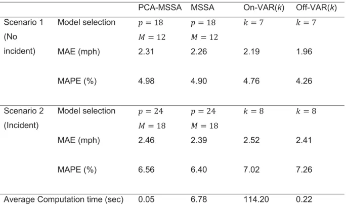
Figure 2-6 Prediction performance of PCA-MSSA and VAR. ... 50

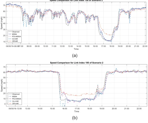
Figure 2-7 Predicted speed profiles: (a) location index 108 and (b) location index 195. ... 52

Figure 2-8 Prediction errors during an incident event. ... 52

(12)

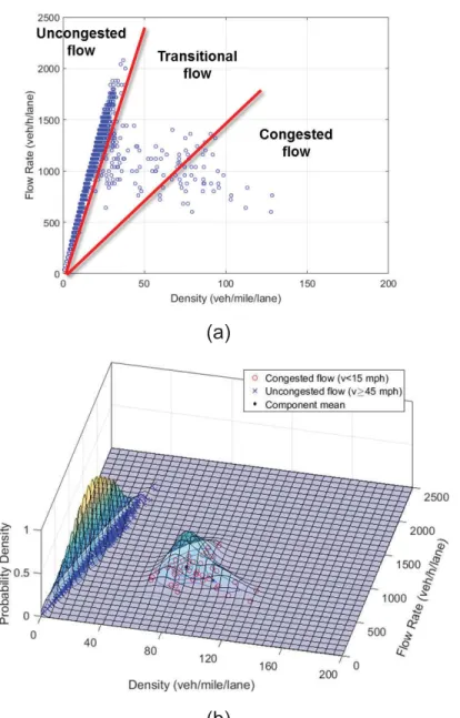
x Figure 3-2 Phase identification: (a) three phases in a flow-density plot and (b) an

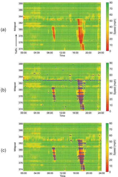
example of estimated data distributions using GMM. ... 68 Figure 3-3 An example of congestion detection (I-40 EB on August 4th_{, 2016): (a)}

speed heat map, (b) congestion detection without filtering, and (c)

congestion detection with filtering. ... 70 Figure 3-4 Flow-density relationship: (a) theoretical flow-density curve and shock

wave speed and (b) real traffic data (station at 374.2 mile EB on August 4, 2016, 4-9 PM). ... 76 Figure 3-5 Shock wave speed calculation: (a) at each station, (b) between two

neighboring stations, and (c) between the first downstream station and each upstream station. ... 76 Figure 3-6 RTMS stations in Knoxville TN. ... 77 Figure 3-7 RTMS speed visualizations for the selected test days. ... 79 Figure 3-8 Phase identification and congestion detection results with speed heat

map: (a) August 4, 2016, (b) August 8, 2016, (c) August 12, 2016, and (d) August 23, 2016. ... 80 Figure 3-9 Phase identification and congestion detection results with speed heat

map: (a) August 30, 2016, and (b) September 1, 2016 (I-40 EB), and (c) September 1, 2016 (I-40 WB). ... 81 Figure 3-10 Congestion detection rate over speeds for each test day. ... 82 Figure 3-11 Shock wave examples based on congestion detection results: (a)

varying capacity, (b) varying demand, and (c) mixed condition. ... 84 Figure 4-1 Contours of control delay for signal control, AWSC, TWSC, and

roundabout with 20% left turns. ... 100 Figure 4-2 Delay surfaces for 4 different control types, with 20% left turns. ... 102 Figure 4-3 Delay surfaces for 3 different control types, with 20% left turns. ... 102 Figure 4-4 Comparison of delay by control types and gray zones with 20% left

(13)

xi Figure 4-5 Comparison of delay by control types and gray zones with 0%, 5%,

10%, 15% left turns. ... 105

Figure 4-6 Comparison of delay by control types with signal optimization and gray zones with 20% left turn. ... 107

Figure 4-7 Comparison of delay by control types with signal optimization and gray zones with 0%, 5%, 10%, 15% left turns... 107

Figure A-1 MCAR patterns and imputed speed. ... 126

Figure A-2 MAR patterns and imputed speed. ... 126

Figure A-3 MNAR patterns and imputed speed. ... 127

(14)

1

INTRODUCTION

Traffic congestion on a highway is one of the most interesting phenomena in traffic management and operations. A great deal of effort has been made to develop and enhance solutions to cope with traffic congestion.

Assessing current traffic conditions and accurately predicting the future in real time are essentials that have not been definitively resolved. Advancement in these capabilities is vital for fast decision making, timely responses, and

appropriate proactive traffic controls to mitigate the impact of congestion on traffic flow.

One purpose of traffic flow analysis is to understand the continuous movement of traffic over time and space. The traffic variables including speed, density, and traffic volume depend on a spatio-temporal domain. Without considering this feature of the data in an analysis, one can make only limited inferences. Thus, more efforts to exploit the spatio-temporal dependency in traffic flow studies are desirable.

Traffic data collected from intelligent transportation systems (ITS) and mobile devices have increased rapidly with significant progress in computing capabilities and data-driven analysis methods. Data sources include conventional traffic data from detectors as well as location-based data from cellphones, car navigation devices, and multiple sensors embedded in connected and

autonomous vehicles. In order to conduct further analysis using these data, one must address a missing data issue. Missing data appears frequently in a real traffic data collection process. This is mainly because collecting data from transportation systems is different from collecting it under well-controlled experimental conditions. If a great deal of data is missing, it can lead to an erroneous analysis.

For traffic flow analysis, the wide variety of sources provides data that represent traffic flow conditions. Speed is one essential type of these data.

(15)

2 Speed is a fundamental variable of traffic flow, and is frequently used for highway capacity analysis, although it is not directly used as a level of service measure. Various traffic phenomena occur in a highway system due to weaving, merging, diverging, and other traffic events that are often measured and explained by speed. Therefore, traffic flow analysis using speed data can provide important information for detecting and predicting traffic conditions.

This dissertation presents studies focused on the development of a traffic flow detection and prediction framework that uses data-driven approaches to support the proactive traffic controls and operations for highways. The

dissertation compiles four research papers in the following chapters. These chapters are organized in a journal article format because each chapter is either published, submitted, or to be submitted.

x Chapter I proposes and evaluates spatio-temporal cokriging methods for missing data imputation in spatio-temporal domain. Different missing data patterns and use of secondary data are considered for enhancing imputation accuracy.

x Chapter II proposes a short-term traffic speed prediction algorithm. A nonparametric time series analysis method with a data dimension reduction technique is evaluated for short-term prediction and compared with a parametric model.

x Chapter III presents a real-time traffic queue detection algorithm based on traffic flow fundamentals using traffic detector data. The queue detection and additional shock wave analysis results are provided using real traffic data.

x Chapter IV introduces gray areas in a decision-making process using a quantifiable performance measure to address uncertainties in modeling output. The gray areas are identified and visualized in a case study of intersection control type selection.

(16)

3

CHAPTER I

MISSING DATA IMPUTATION FOR TRAFFIC SPEED USING

SPATIO-TEMPORAL COKRIGING

(17)

4 This chapter presents a modified version of a research paper by Bumjoon Bae, Hyun Kim, Hyeonsup Lim, Yuandong Liu, Lee D. Han, and Phillip B. Freeze.

Abstract

Modern transportation systems rely increasingly on the availability and accuracy of traffic detector data to monitor traffic operational conditions and assess system performance. Missing data, which occurs almost inevitably for a number of

reasons, can lead to suboptimal operations and ineffective decisions if not

remedied in a timely and systematic fashion through data imputation. A review of the literature suggests that most traffic data imputation studies considered the temporal continuity of the data but often overlooked the spatial correlations that exist. Few of the studies explored the randomness of the patterns of the missing data. Therefore, this paper proposes two cokriging methods that exploit the existence of spatiotemporal dependency in traffic data and employ multiple data sources, each with independently missing data, to impute high-resolution traffic speed data under different data missing pattern scenarios. The two proposed cokriging methods, both using multiple independent data sources, were benchmarked against a classic ordinary kriging method, which uses only the primary data source. An array of testing scenarios were designed to test these methods under different missing rates (10~40% data loss) and different missing patterns (random in time and location, random only in location, and non-random blocks of missing data). The results suggest that using multiple data sources with the spatiotemporal simple cokriging method effectively improves the imputation accuracy if the missing data were clustered, or in blocks. On the other hand, if the missing data were randomly scattered in time and location, the classic ordinary kriging method using only the primary data source can be more effective. Our study, which employs empirical traffic speed data from radar

(18)

5 detectors and vehicle probes, demonstrates that the overall predictions of the kriging-based imputation approach are accurate and reliable for all combinations of missing patterns and missing rates investigated.

Introduction

Traffic detector data collected from transportation facilities are essential inputs for modern transportation systems to monitor traffic conditions and assess system performance. A challenge for using the data is ‘missingness’ in the data

collection processes of the systems [1, 2]. This includes (but is not limited to) the malfunctions of hardware or software, communication network problems,

restricted power supply conditions, scheduled maintenance, and so on. As Orchard and Woodbury [3] remarked, it is obvious that not to have missing data is the best way to address the missing data issue; however, this ideal

circumstance rarely happens.

The effects of missing data and imputation methods have been examined in other disciplines, such as statistics, sociology, and epidemiology because analysis results are considered rough when data are missing [1]. Unfortunately, this issue has not been well addressed in transportation studies [4, 5]. Measuring the effects of missing data and treatments to impute them are rarely investigated, even though the issue of handling missing data has been addressed to some degree in transportation modeling. Meanwhile, the need to measure the

performance of transportation systems such as delay, travel time reliability, and emissions has been underlined in transportation systems management and operations. In this context, the appropriate methods to impute missing data should be explored, otherwise, the results of such performance measures will be biased.

(19)

6 The effects of missing traffic flow data on transportation modeling and prediction can be divided into two categories [6]: First, it causes information loss for certain locations and time periods, which may be important to the objective of an analysis in transportation modeling and prediction. For instance, if traffic speed and traffic volume data are missing for a severely congested road segment during peak hours, the total vehicle emission will be underestimated. Second, it causes statistical information loss. In general, a sample size that is smaller due to missing data, i.e., smaller degrees of freedom, may lead to overfitting problems in the modeling process. More importantly, underlying

assumptions of statistical methods used in an imputation analysis are violated by different missing patterns, resulting in biased solutions.

Therefore, to avoid erroneous statistical inference, understanding missing patterns and missing mechanisms from the datasets used in a statistical analysis is as important as determining how to sample from a population. Rubin [7] points out that distributional inferences on the parameters of data are generally

conditional on the observed missing patterns. According to recent works by Buuren [1] and Carpenter and Kenward [2], a typology of missing patterns associated with the impact on statistical analysis are identified with three types: missing completely at random (MCAR), missing at random (MAR), and missing not at random (MNAR). Few of previous studies explored the randomness of the patterns of the missing traffic flow data, but not fully investigated these missing patterns [8-11].

Imputation of traffic data such as volume, speed, and occupancy collected from traffic detectors aims to estimate the unobserved value at a specific location and time to improve the accuracy of further analyses (traffic speed prediction, traffic incident detection, and so on). Recent transportation studies paid attention to a geostatistical approach, called kriging, to estimate or predict traffic variables for unobserved locations [12-16]. Considering that traffic data have

(20)

7 approaches for improving imputation accuracy. This is because the method takes the observed neighboring data correlated with a missing value into account in space-time dimension. A recent kriging study extends the modeling dimension from a single spatial dimension to a spatiotemporal dimension to impute traffic speed data, arguably suggesting that spatiotemporal-kriging (ST-Kriging)

outperforms the historical average and k-nearest neighborhood (KNN) methods [17].

The goal of this study is to extend the ST-Kriging approach to a multivariate framework (called spatiotemporal cokriging) for imputing high-resolution traffic speed data collected from Remote Traffic Microwave Sensors (RTMS) on highways. As cokriging is inherently the multivariate extension of kriging [18], cokriging needs to input the secondary variables to complement the observed neighboring values of the primary variable to predict the value of a primary variable at a new location. The secondary variables are spatially

correlated with the primary variable. Because available traffic data resources are abundant, using the information from multiple data sources is anticipated to improve the imputation results of the spatio-temporal cokriging approach. The effectiveness of cokriging relies on the pattern of missing data. To address this issue, we investigated the prediction performance of three different kriging

methods based on three missing patterns (MCAR, MAR, and MNAR) in the traffic speed data.

The next section presents a comprehensive literature review on imputation techniques and kriging in transportation studies and describes the data used in this study. The following section explains the kriging and cokriging methods. The last two sections provide a case study result of applying the spatiotemporal cokriging approach to impute traffic flow speed data, then conclusions follow.

(21)

8

Literature Review

Missing data imputation methods can be either single imputation or multiple imputation [1, 2]. Hot-deck, average, and regression are commonly used as single imputation methods. Most of the imputation studies in transportation

examine single imputation methods because of their fast-computational speed for real-time analysis. The historical average, expectation maximization (EM)

algorithm [4], pairwise regression [19], moving average, ARIMA, and regression model with genetic algorithm [20] have been explored for imputing five or 10 minutes loop detector data.

In contrast, multiple imputation methods overcome the drawback of single imputation methods that derive standard errors of parameter estimates that are too small. This type of imputation generates multiple imputed datasets and estimates model parameters, then pools the estimates as a single value. Thus, it can deal with the inherent uncertainty of the imputations [1]. Ni and Leonard Ii [5] proposed a multiple imputation approach employing a Bayesian network and Markov chain Monte Carlo (MCMC) technique with 20-second detector data. The imputation method can account for the correlations between and within variables by using a Bayesian network to produce unbiased estimates and confidence intervals of the results from the MCMC. However, these studies exploited only time series information of the traffic data at the location of interest or the traffic data of closest surrounding detectors, which are selected arbitrarily on the basis of spatiotemporal relationship assumed in advance.

Recent studies have focused more on both the spatial context of traffic data as well as temporal patterns [9, 11, 21]. Clearly, analyzing traffic dynamics in the context of space and time is useful since traffic status evolves in the spatiotemporal domain. Thus, efforts have been made to visualize and analyze traffic data projecting in three or more dimensions, including space and time [21, 22]. Spatiotemporal properties of traffic detector data were also explored using a

(22)

9 cross-correlation analysis [23]. The results can be used to identify the influential area of a missing data point in a spatiotemporal domain.

Kriging is a well-known geostatistics interpolation method developed by D. G. Krige [24] to estimate a value at an unobserved location from observations at nearby locations. Previous transportation studies exploring kriging methods were focused on estimating annual average daily traffic (AADT) for unobserved

locations. Eom, Park [12] employed kriging to impute missing AADT data. In comparison with an ordinary least square (OLS) regression model, the kriging approach predicted AADT more accurately. Kriging was also used to predict future AADT with temporal extrapolation by OLS regression [13]. The study showed that kriging approaches perform better for road sections with moderate-to-high traffic volumes. Under low traffic demand conditions, the proposed kriging method overestimates AADT. Since the spatial covariance considered in kriging is based on Euclidean distance between two locations, Zou, Yue [14] proposed an approximated road network distance, which is a Euclidean distance and approximately equal to the road network distance using isometric embedding theory. Therefore, the metric can be used for the traditional kriging and its covariance function. In comparison with the Euclidean distance, the proposed distance metric performed better for interpolating travel speed using local universal kriging, especially for a region with a complex road network structure. However, Selby and Kockelman [15] showed that using network distances, instead of Euclidean distance, did not significantly improve the prediction

performance of a universal kriging method for AADT prediction. Shamo, Asa [16] compared three different kriging methods—simple kriging (SK), ordinary kriging (OK), and universal kriging (UK)—to predict AADT in Washington State in U.S. over a period of three years. The result showed that there is no superior kriging method from year to year due to the dynamic nature of traffic volume. Meanwhile, there are attempts to extend the spatial analysis dimensions of kriging to a

(23)

10 various disciplines [17, 25, 26]. However, there is virtually no available literature associated with imputation and prediction modeling. Given the theoretical

advantage of cokriging, applying cokriging method to impute missing traffic data is promising in case any secondary data that are highly correlated with a primary data are available. Since multiple traffic speed data sources are available, it is worthwhile to explore the applicability and performance of cokriging for traffic data imputation.

Data Description

The primary data to be imputed in this study was obtained from the RTMS, monitored by roadside sensors in the Knoxville urban area; Knoxville is the third largest city in Tennessee. There are more than 200 detector stations for both directions on the interstates, including two major highways in the Knoxville region, I-40 and I-75. Figure 1-1 shows the selected RTMS station locations together with the station ID labels. Twenty-eight stations in the 13.6 mile-long eastbound I-40 segment, ranging from mile marker 374.2 (west end) to 387.8 as (east end), were selected because it is a major city corridor. Along with Figure 1-1, Table 1-1 summarizes the selected RTMS stations that are aligned to 12 links of the secondary dataset, called HERE on I-40 Highway in Knoxville, TN. There were 5,881 cases where both speeds were collected at the same spatiotemporal point.

RTMS collects traffic count, speed, and occupancy information for each lane every 30 seconds. Speed is the essential variable for measuring the performance of the highway system in terms of travel time reliability, delay, emissions, and so on. To explore the cokriging approach for data imputation, the five-minute average speed data for 24 hours were collected on December 1, 2015. This gave a total of 288 observations for each station if no missingness

(24)

11 Figure 1-1 Map of the selected RTMS stations on I-40 eastbound in

(25)

12 Table 1-1 Description of RTMS stations and corresponding HERE links.

RTMS HERE

Station

ID Mile Marker Direction Link ID Link Length (mile)

3 374.2 Eastbound 121P04124 2.0 4 374.5 Eastbound 6 374.9 Eastbound 9 375.4 Eastbound 121P04125 1.2 11 375.9 Eastbound 13 376.2 Eastbound 14 376.6 Eastbound 121P04126 0.5 17 377.1 Eastbound 121P04127 1.3 19 377.5 Eastbound 21 378.0 Eastbound 23 378.4 Eastbound 121P04128 0.5 27 379.2 Eastbound 121P04130 0.8 33 380.4 Eastbound 121P04131 1.2 34 380.7 Eastbound 38 381.5 Eastbound 121P04132 2.3 40 381.9 Eastbound 41 382.2 Eastbound 43 382.6 Eastbound 48 383.6 Eastbound 121P04133 1.3 52 384.4 Eastbound 54 384.7 Eastbound 121P04144 0.8 56 385.1 Eastbound 58 385.4 Eastbound 61 386.1 Eastbound 121P04146 0.5 64 386.5 Eastbound 65 387.0 Eastbound 67 387.5 Eastbound 121P04149 0.2 68 387.8 Eastbound

(26)

13 occurred. The main reason to use five-minute data is for consistency with the aggregation scale of the secondary data used in this study. Note that the raw data were collected in 30 seconds interval; however, it was aggregated to remove the effect of unnecessary noise as it is prone to a biased distribution for imputation in our study. In our examination, the aggregation of the raw data at five-minute intervals was considered a reasonable time span for imputation. The secondary data used in the cokriging method called HERE is a commercial link-based speed dataset collected mainly from probe vehicles. As mentioned, this data contains traffic speeds averaged in five minutes, totaling 288 observations per day for each road link. The HERE data were obtained at the same road segments on the same date of the RTMS dataset. Note that the RTMS dataset is point-based while the HERE dataset is link-based. Thus, to match the RTMS station locations with the links of HERE, a geographic information system (GIS) tool was used for the data matching allocation.

In each dataset, the number of complete data points for a day should be 8,064 (=28 stations ൈ288 per day for five-minute interval). However, the obtained

RTMS dataset had 6,954 observations and the HERE dataset contained 6,817 observations, presenting the original missing rates of both RTMS and HERE samples in this study are 13.8% and 15.5%, respectively. Figure 1-2 shows the scatter plots of the RTMS (Figure 1-2(a)) and HERE (Figure 1-2(b)) observations in spatiotemporal dimension. Most of the missing values in the HERE data are observed at nighttime because HERE data are collected from probe vehicles that operate mostly in the daytime. Nevertheless, the HERE data are still useful for daytime analyses. In terms of missingness in the RTMS data, the missing pattern is a random pattern.

Given the obtained dataset, two assumptions are made to use the RTMS and HERE data together. First, five-minute aggregated data from the original 30-second RTMS are used for the consistency of the temporal scale of HERE. Consequently, the changes within five minutes of the raw RTMS data are

(27)

14 Figure 1-2 Collected five-minute average speed points: (a) RTMS and (b) HERE. Each dot represents an observation point in spatiotemporal dimension.

(28)

15 smoothed. This pre-processing has an advantage because the aggregation can reduce the impact of the noise in the raw data and improve computation

efficiency [5]. Second, the resolution and accuracy of the secondary data, HERE are assumed to be sufficient to explain a part of the variation in the primary data within the proposed cokriging imputation framework. It is expected that the HERE data be helpful to impute missing RTMS values because the completeness rate of HERE is well established during daytime collection.

Methodology

Since kriging was first developed as an interpolation technique for geographical surfaces, it has become a representative geostatistical approach to predict an unknown value at an unobserved location by adapting various statistical assumptions and conditions in the modeling and has further advanced to

different kriging methods. The interpolation was formulated as a weighted sum of the values of their known neighbors. In this study, the speed at an unobserved location is estimated using three different kriging methods: ordinary kriging (OK), ordinary cokriging (OCK), and simple cokriging (SCK).

OK is the most commonly used kriging method [27]. With local second-order stationarity assumption, OK is known as the best linear unbiased estimator (BLUE). In this study, the speed at an unobserved location ࢙଴ is calculated from a

linear combination of the observed speed ܸሺ࢙_ఈሻ at neighboring locations and its weight ߣ_ఈ: ܸכ_ሺ࢙ ଴ሻ ൌ ෍ ߣఈܸሺ࢙ఈሻ ௛ ఈୀଵ ሺͳሻ

where, ࢙_ఈ is a vector of the location where an observed RTMS speed ܸ is placed on a spatiotemporal plane, ࢙଴ is a vector of the location where unobserved RTMS

(29)

16 speed ܸכ will be predicted, and ݊ is the number of observed locations used for prediction. To obtain an unbiased estimate, the following constraint is added:

෍ ߣ_ఈൌ ͳ

௛

ఈୀଵ

ሺʹሻ

OCK is a multivariate extension of OK. Using OCK, secondary variables can be added to predict a primary variable. OCK can be expressed as follows:

ܸ_௜כ_బሺ࢙଴ሻ ൌ ෍ ෍ ߣఈ௜ ܸ௜ሺ࢙ఈሻ ௛೔ ఈୀଵ ௄ ௜ୀଵ ሺ͵ሻ

where, ܸ_௜כ_బ is unobserved speed of a primary variable, RTMS to be predicted and ܭ is the number of variables, and ݄_௜ is the number of observed locations of ݅th variable. A similar but conditional constraint of OK is added in OCK:

෍ ߣ_ఈ௜ ௛೔

ఈୀଵ

ൌ ቄͳ݅ ൌ ݅଴

ͲǤ ሺͶሻ

Then, the main difference between OCK and SCK is how the mean value is specified for interpolation. A constant global mean is used in SCK, while the

local mean is used in OCK, which varies depending on each set of neighboring

data points. Therefore, the accuracy of the OCK-based prediction could decrease when no neighborhood data are available. Under such conditions, SCK is more useful since an estimation of a primary variable can be calibrated without having neighboring primary data [27]. SCK is expressed as:

ܸ_௜כ_బሺ࢙_଴ሻ ൌ ݉_௜_బ ൅ ෍ ෍ ߣ_ఈ௜ _ሾܸ ௜ሺ࢙ఈሻ െ ݉௜ሿ ௛೔ ఈୀଵ ௄ ௜ୀଵ ሺͷሻ

(30)

17 where, ݉_௜_బ is the global mean of a primary variable, and ݉_௜ is the global mean of

݅th variable.

In kriging, the spatial dependency between two locations is analyzed by covariance or semivariogram where Euclidean distance between the observed data at any pair of locations is used to generate a best-fit semivariogram.

Complete details about the semivariogram functions and underlying assumptions are available in Cressie [28], Eom, Park [12], and Zou, Yue [14]. As shown in Figure 1-2, time and space are represented with two dimensions. Notice that a road section is represented as a straight line in the Y-axis, and the observed locations are placed on the line scaled by their mile marker. Each data point was mapped on the grid in which each cell size is five-minute by 0.1-mile. Similar to what Zou, Yue [14] did, this design makes the network distance equal to the Euclidean distance, allowing the computation of spatial dependency to be more accurate and the visualization of results more effective.

Figure 1-3 presents the procedure of the analysis design: (a) collecting and preprocessing RTMS and HERE data, including map matching and data extraction and aggregation; (b) analyzing the correlation between RTMS and HERE speed data, which is for verifying that HERE is an appropriate secondary variable; (c) generating three missing patterns in the collected RTMS data; (d) creating experimental semivariogram of both data and fitting theoretical

semivariogram; (e) predicting the missing RTMS speeds and mapping the spatiotemporal distribution; and (f) evaluating the accuracy of the results of OK, OCK, and SCK given the missing patterns.

Analysis Results

Correlation analysis

In order to justify the use of HERE as the secondary variable for imputing the RTMS data using cokriging, we carried out correlation analysis between two

(31)

18 Figure 1-3 Research design.

(32)

19 datasets. Pearson correlation coefficient (r) was used as Eq. (6).

ݎ ൌ σ ሺݔ௜ െ ݔҧሻሺݕ௜െ ݕതሻ ௡

௜ୀଵ

ሺ݊ െ ͳሻݏ௫ݏ௬

ሺ͸ሻ

where, ݔ is RTMS, ݕ is HERE, ݊ is sample size (n = 5,881), and ݏ is a sample standard deviation of each data. As shown in Figure 1-4(a), the correlation between RTMS and HERE is 0.46. However, by taking log-transformation in Figure 1-4(b), the correlation is improved to r = 0.51. Empirically, this correlation is enough to justify taking the additional complexity of cokriging into account since it is known that cokriging results in better predictions than ordinary kriging if the correlation between two variables exceeds 0.5 and when a secondary

variable is over-sampled [29, 30]. Most of the speed observations in both data are near 60 miles per hour (mph) and they seem to have a relatively low correlation, i.e., the cluster near 60 mph has a circular shape in Figure 1-4(a). This is mainly because of the resolution difference between both data. In other words, one HERE link covers up to 4 RTMS stations in this study. However, low speed below the free flow speed of near 60 mph is generally more important in an analysis for traffic flow since congestion represented by low speed is one of the most interesting phenomena in transportation studies. In that perspective, the low speed observations in both data show a linear relationship, which supports that HERE is an appropriate secondary data for imputing the missing RTMS data.

Design of scenarios for missing patterns

The definitions of three missing patterns – MCAR, MAR, and MNAR, are as follows: (a) the probability of a value missing at a certain location and time is completely independent in MCAR. (b) In MAR, missingness is dependent on a certain condition, but independent within the condition [1]. (c) MNAR represents the pattern that a missing mechanism is neither MCAR nor MAR. Using three

(33)

20 Figure 1-4 Scatter plots between RTMS and HERE: (a) original speed, and (b) log-transformed speed.

(34)

21 missing patterns, a total of 12 missing scenarios were generated by four missing rates from 10% to 40% in increments of 10%. In MCAR scenarios, a portion of the individual data points was removed completely at random in time and

location. In MAR scenarios, series of the data points were removed for randomly selected stations and time periods to satisfy the condition that the missingness is dependent on time, but not on locations. In MNAR scenarios, a set of data points in a block was eliminated from original data to generate a different pattern

compared to MAR and MCAR. Figure 1-5 shows three examples of the RTMS scatter plot given missing patterns with a scenario of 10% missing rate.

Semivariogram modeling

Using the Geostatistical Analyst tool in ArcGIS 10.4, experimental

semivariograms were computed, then theoretical semivariograms were estimated for OK, OCK and SCK. Note that no dominantly superior semivariogram model has been suggested for each of the three kriging methods for traffic flow data prediction and imputation in existing literature [16, 31], implying the best fitted semivariogram model needs to be designed depending on the data used in the cases. However, recent works by Shamo, Asa [16] and Yang [31] argued that spherical and exponential models could outperform others with traffic flow data from their empirical observations. In our study, the spherical model was fitted best in our case, thus, it was applied for three kriging methods to maintain consistency in comparing them.

The HERE speed was used as the secondary variable in both cokriging methods (OCK and SCK). A theoretical semivariogram model measuring spatial

dissimilarity of any pair of observations consists of three parameters: nugget (the minimum estimate of error), sill (the maximum dissimilarity), and range (the distance to reach to sill). Note that it is necessary to find the best fitting

semivariogram for both data to set the equation of selected kriging methods that are best solvable in imputation. Figure 1-6 shows the best-fitted theoretical

(35)

22 Figure 1-5 Missing scenario plots with 10% missing rate: (a) MCAR, (b) MAR, and (c) MNAR. Each dot represents observation point in

(36)

23 Figure 1-6 Theoretical semivariograms: (a) OK, (b) OCK, and (c) SCK.

(37)

24 semivariograms of the three kriging methods. The process to identify the best-fitting theoretical semivariogram over experimental semivariogram is difficult if greater variability is present in the pattern of binned cloud [27, 28]. To tackle this issue, the log-transformation was applied to HERE data in OCK and the RTMS and HERE data were transformed as normal scores in SCK. This is because simple kriging requires the assumption that the true mean of data must be known, which is identified as the best theoretical semivariogram for SCK [32]. Evaluation of the results

Given the missing patterns scenarios, a total 36 RTMS speed surfaces were generated to evaluate the imputation performance of the three kriging methods. Figure 1-7 is provided as reference patterns of the RTMS and HERE datasets (Figure A-1, Figure A-2, and Figure A-3 show the imputation results in Appendix). The removed observations in each analysis were used as ground truth for

individual missing values. Note that the original missing RTMS values were not accounted for in the evaluation because their true values are not available. In order to evaluate imputation performance of OK, OCK, and SCK, mean absolute

error (MAE) and mean absolute percentage error (MAPE) were used. Both

measurements are formulated as follows:

ܯܣܧ ൌ ͳ ݊෍หܸ௜ െ ܸ෠௜ห ௡ ௜ୀଵ ሺ͹ሻ ܯܣܲܧ ൌ ͳ ݊෍ หܸ_௜െ ܸ෠_௜ห ܸ_௜ ௡ ௜ୀଵ ൈ ͳͲͲ ሺͺሻ

where, ܸ_௜ is the ݅th observed RTMS speed and ܸ෠_௜ is the ݅th predicted RTMS speed.

(38)

25 Figure 1-7 Imputed Speed using OK without missing values: (a) RTMS and (b) HERE.

(39)

26 The six plots in Figure 1-8 present the prediction performance of the three kriging methods under different missing data patterns and rates (The same results are presented in Table A-1 in Appendix).

For the MCAR scenarios depicted in Figure 1-8(a) and Figure 1-8(b), where data are missing completely at random, ordinary kriging (OK) clearly outperforms the others. Since plentiful of neighboring RTMS data are present near each missing point in both space and time domains in the MCAR scenario, the availability of neighboring HERE data points does not contribute meaningfully to the imputation effort. Despite the different performances among the three kriging methods, the error range of 1.9 – 3.2 mph, which can be ignored for imputation, confirms that kriging is an effective tool for missing data imputation if a missing pattern

presents with a form of MCAR. Figure 1-8(a) and Figure 1-8(b) indicate that kriging-based imputation can provide reliable results for the MCAR pattern. The performance of three kriging approaches is consistently stable with varying missing rate. Notice that a single data based kriging imputation (OK) provides a

“good” result when supplementary data would play as a role of noise in MCAR.

However, it is worth noting that the MCAR pattern is less likely to occur in real traffic detector data.

The prediction errors of the MAR scenarios are shown in Figure 1-8(c) and Figure 1-8(d); the mean error (left) and mean percentage error (right) on average are 5.4 mph and 11.2%, respectively, both of which are higher than the ranges of MCAR results. The main reason for this result is that the missing values are more clustered as a form of time series in the scenarios compared to MCAR. This result concurs with the argument that temporal dependency of traffic detector

data is stronger than spatial dependency, as proposed by Wang and Kockelman [13]. Another feature in the MAR pattern is that there is no distinct difference in the prediction errors among the three kriging methods. In

(40)

27 Figure 1-8 MAE and MAPE comparisons.

(41)

28 there are a smaller number of neighboring RTMS data points explaining the temporal dependency.

In the MNAR scenarios in Figure 1-8(e) and Figure 1-8(f), simple cokriging (SCK) outperforms the others, and the gaps in the error measures are much greater than those in the previous two missing patterns. The mean error of SCK ranges from 4.7 to 6.5 mph, while that of OK and OCK ranges from 9.4 to 11.4 mph. Likewise, the range of the mean percentage error of SCK is from 9.3% to 12.4%, while that of both ordinary kriging methods (OK and OCK) is from 16.1% to 21.0%. The prediction performances of OK and OCK are very similar in the MNAR scenarios. As discussed in the previous section, both ordinary kriging methods use an unknown local mean of a set of neighboring data points. In other words, the accuracy of the predicted value for OK and OCK could be lower than that of SCK when there are fewer or no reliable neighboring values. Since a block of data points was removed in the MNAR scenarios, the remaining neighboring data points are not as good as those in the previous two missing pattern scenarios for explaining the spatiotemporal dependency. Similar to the implication of MAR, the utility of cokriging approaches that take secondary

variables into account for predicting unknown primary values is regarded as more effective when missing values are clustered over a relatively extensive

spatiotemporal domain.

Given our experiments, it is clear that the prediction errors of the MNAR scenarios decrease gradually as missing rate increases. This is mainly because the proportion of high-speed observations in the validation dataset of a higher missing rate scenario increases. Since these high-speed observations are similar to the mean of the RTMS data used in this study, the overall imputation error decreases as the size of missing block increases, consequently.

(42)

29

Conclusion

Most of the traffic flow data imputation studies in the past have focused on investigating imputation techniques with a single data source. However, by increasing the number of data collecting sensors and other technologies over the last decade there are abundant alternative data sources that can be used to complement each other, suggesting the potential to use multi-source data to enhance imputation for missing traffic flow data. To this end, this study proposed a spatiotemporal cokriging approach to impute high resolution traffic speed data by using two complementary data sources, RTMS and HERE speed data. Two cokriging methods, ordinary and simple, were used and evaluated by comparing them with the spatiotemporal ordinary kriging method. The radar detector data (RTMS) and probe vehicle data (HERE) were used for the cokriging-based imputation approaches as primary and secondary variables, respectively.

Three different missing patterns in the spatiotemporal domain with varying missing rates were tested to evaluate the prediction performances of the

cokriging methods. Generally, all kriging methods provide reliable and consistent results over various missing rate under the MCAR patterns (random in time and location) with very small, negligible errors. Because sufficient highly correlated neighboring data points exist for each missing value in the spatiotemporal

context, the prediction performance is hardly influenced by missing rates. Among the three methods, ordinary kriging outperforms the others. For MAR patterns (random only in location), the difference in the performances of all methods is not prominent. For this reason, using only a primary data source for MCAR and MAR patterns can be more cost-effective than using multiple data sources. Meanwhile, one possibility of improving the prediction performance of cokriging is to consider secondary data sources if they are highly correlated with the primary data. In this study, each HERE data link covers multiple RTMS stations, implying the lower resolution of the secondary variable and relatively weak correlation between two

(43)

30 data sources. This may cause the cokriging methods to have the test errors. Nevertheless, it was underlined that using secondary data sources with the simple cokriging can improve prediction results when the missing pattern follows MNAR (not random in time and location). Traffic flow data collected from

detectors on roads usually have missing values for a variety of reasons.

Considering the fact that traffic detector data may be missing because of system malfunctions, no power supply, and maintenance, the patterns are likely to be MAR or MNAR and using spatiotemporal cokriging with multiple data sources can be beneficial for imputation.

(44)

31

CHAPTER II

SHORT-TERM TRAFFIC SPEED PREDICTION FOR A

LARGE-SCALE ROAD NETWORK

(45)

32 This chapter presents a modified version of a research paper by Bumjoon Bae, and Lee D. Han.

Abstract

Short-term traffic prediction has been an essential part of real-time applications in modern transportation systems for the last few decades. Despite the recent progress in the voluminous models and data sources, many existing studies have focused on prediction for either a single or a few locations. In addition, the spatio-temporal dependency in the traffic data was narrowly accounted for. Therefore, this paper proposes a new short-term traffic speed prediction algorithm that can efficiently cope with the complexity and immensity of the prediction process derived from the network size and amount of data in order to provide accurate predictions in real time. This algorithm consists of two modules: (a) principal component analysis (PCA) for data dimensionality reduction and feature

selection, and (b) multichannel singular spectral analysis (MSSA) for multivariate time-series data prediction. A large amount of traffic data is efficiently

compressed by PCA with high accuracy, then used as an input in the

nonparametric multivariate time-series analysis. The algorithm was compared with a vector autoregressive (VAR) model to predict traffic speeds five minutes ahead for a 21.3 mile-long highway segment, using the traffic detector data, and for 451 mile-long segment, using probe-based speed data in Tennessee. The proposed algorithm is found to provide accurate predictions with a computation time of less than one second without training. Furthermore, the proposed algorithm shows a better prediction performance under congested flow conditions, compared to VAR. This indicates that the proposed algorithm is suitable for real-time prediction and scalable for a large network analysis.

(46)

33

Introduction

Traffic speed is one of the fundamental variables that characterize traffic flow. It is not only a traffic performance measurement of roadway systems, but also an input for estimating other measurements such as travel time, vehicle emission, traffic noise, and so on [33]. Hence, traffic speed prediction is a core function required in modern traffic management and operation systems. In the last few decades, various short-term traffic speed prediction models and algorithms have been developed for real-time intelligent transportation systems (ITS) applications.

Although there is no absolute definition of how long the ‘short-term’ is, the prediction time step varies from one second to five minutes in the literature [34-42]. And the prediction horizon has been set as the range from one minute to two hours in advance through multi-step runs [43]. According to a recent

comprehensive review on short-term traffic forecasting by Vlahogianni, Karlaftis [43], the majority of the previous studies used univariate models with traffic detector data at a single location on a highway. Statistical time-series models and neural network (NN) type models present a noticeable frequency of use. The time-series models include vector autoregressive (VAR) models for multivariate prediction [38, 39], spatial temporal autoregressive moving average (STARMA) for considering spatiotemporal correlation [41], generalized autoregressive

conditional heteroscedasticity (GARCH) for capturing unexpected speed dynamic shifts [40], and adaptive Lasso regression for improving prediction performance by minimizing error variance [44], and so on. On the other hand, a variety of NN based models has also been proposed for speed prediction. These models are known to provide a more accurate prediction for nonlinear traffic flow compared to the classical statistics models [45-47]. Further, these models have been tested with Kalman filters or wavelet transformation technique primarily for denoising traffic data [37, 48, 49].

(47)

34 In the literature, the mean absolute prediction error (MAPE) of existing studies ranges from 2.5% to 15.0% for five-minute predictions [34, 35, 37, 38, 41, 44, 45, 49]. Although the effects of variability in the time step on prediction

performance has not been addressed sufficiently, the prediction error shows generally a linear association with the length of a prediction time step or the number of time steps increase [34, 35, 41, 44, 50]. A few studies compared the prediction performances of congested and non-congested traffic flow conditions. They showed that the prediction errors of congested conditions are

approximately three times higher than those of non-congested conditions [38, 40]. The speed threshold to define congestion varies over the studies, ranging from 30 miles per hour (mph) to 40 mph.

Despite the extensive studies on short-term traffic speed prediction, few have attempted to address the following limitations. The existing studies applied five minutes as a prediction time step without considering its effects. This is mainly because five minutes had been used most frequently in literature and the available data resolution was five minutes. Furthermore, there was insufficient information in the literature on computation time evaluation as real-time

applications, which is helpful for other researchers and practitioners. In addition, many of the previous studies have been done on the short-term prediction for a single or several locations, in which a spatio-temporal dependency of traffic data was not sufficiently considered.

This paper proposes a new short-term traffic speed prediction algorithm for a large-scale road network. To support real-time and proactive traffic

operations, the proposed algorithm aims to predict the future traffic flow

conditions accurately and quickly without training a model. It is a nonparametric and data-adaptive algorithm that can handle a large-scale spatiotemporal speed data within a short amount of time.

The remainder of this chapter is in this manner. The next section details the methodologies used in the proposed algorithm. Then, the data sources and

(48)

35 different aspects of testing performance are described. Next, the prediction

performance of the proposed algorithm is compared with that of vector

autoregressive (VAR) model that has been successful in the past 10 years [38, 39, 43]. Finally, a discussion on the results and conclusion are drawn.

Methodology

The proposed algorithm consists of principal component analysis (PCA) and multichannel singular spectrum analysis (MSSA) (see Figure 2-1). First, PCA is used to extract features and reduce dimensions of the data. Then, MSSA is used for multivariate time-series prediction using the principal components from PCA. This approach has achieved satisfactory performance in medical image

processing studies [51, 52].

Unlike the statistical prediction models such as autoregressive integrated moving average (ARIMA), MSSA, a multivariate extension of singular spectrum analysis (SSA) is a nonparametric, data-adaptive time-series analysis method that does not require any assumptions, such as stationarity of the data, linearity of the model, or normality of the residuals [53, 54]. These features make MSSA useful [53, 55-57]. Hence, SSA and MSSA have been widely applied recently in many disciplines such as economics, medical image processing, climatology research, etc. [51, 58, 59]. More theoretical and mathematical details of SSA can be found in [57] and [60]. Furthermore, using the principal components (PC) as an input of MSSA allows the prediction to be made based on spatio-temporal dependencies in the data. According to Asif, Kannan [61], PCA consistently provides high reconstruction accuracy over different compression rates for spatiotemporal traffic data.

(49)

36 Figure 2-1 Proposed speed prediction algorithm.

(50)

37 Principal Component Analysis (PCA) for Data Dimension Reduction and Feature Extraction

Principal component analysis (PCA) is a widely used multivariate statistical procedure used for data dimension reduction and feature extraction [62]. It is an orthogonal transformation method that projects the original data onto the spaces of linearly uncorrelated variables where the variance is maximized based on eigenvalues and eigenvectors. Therefore, the principal components (PC), the transformed data can be used as an input for a variety of post analyses.

The speed observation ݔ_௜௧, ͳ ൑ ݅ ൑ ݊, ͳ ൑ ݐ ൑ ݌, with ݅ representing location and ݐ representing time, gives the multivariate time-series data as

ܺ ൌ ൥

ݔ_ଵଵ ڮ ݔ_ଵ௣

ڭ ڰ ڭ

ݔ௡ଵ ڮ ݔ௡௣

൩ ሺͻሻ

The covariance matrix is calculated as

ܥ ൌͳ ݌෍ ߖ௧ߖ௧ ் _{ൌ ߔߔ}் ௣ ௧ୀଵ ሺͳͲሻ

where, Ȳ_௧ൌ ܺ_௧െ ߤ, which is the vector difference between the observations at time ݐ and the mean of ܺ, ߤ. Since ߔ ൌ ଵ

ξ௣ൣߖଵǡ ǥ ǡ ߖ௣൧, the dimension of the

covariance matrix ܥ is ሺ݊ ൈ ݊ሻ.

As the road network size to be analyzed is increased, especially when ݊ ب ݌, calculating ߔߔ் and its eigenvectors becomes more intractable. In order to near-real-time analysis, Turk and Pentland [63] proposed to use ߔ்ߔ instead of ߔߔ், which reduces the dimension from ሺ݊ ൈ ݊ሻ to ሺ݌ ൈ ݌ሻ. This approach is very common in image processing analysis where the input data at each time step is usually a 2-dimentional image. For example, if the input data size is

(51)

38 covariance matrix. More details about the relationship of ߔ்ߔ with ߔߔ் is

provided in Equation (11) through Equation (14). The eigenvector ݒ௜ is defined as

ߔ்ߔݒ௜ ൌ ߣ௜ݒ௜ ሺͳͳሻ

where, ߣ_௜ is the eigenvalue of ߔ்_ߔ_{denoted by}_ߣ

ଵ ൒ ڮ ൒ ߣ௣. If ߔ is multiplied in

both sides of Equation (11),

ߔߔ்_ߔݒ

௜ ൌ ߣ௜ߔݒ௜ ሺͳʹሻ

and using Equation (10) and Equation (12),

ܥߔݒ_௜ ൌ ߣ_௜ߔݒ_௜Ǥ ሺͳ͵ሻ

Then, Equation (13) can be expressed as

ܥݑ_௜ ൌ ߣ_௜ݑ_௜Ǥ ሺͳͶሻ

Therefore, ߔߔ் and ߔ்ߔ have the same eigenvalues and their eigenvectors have the relationship as ݑ௜ ൌ ߔݒ௜.

Finally, the orthogonally transformed data, ܻ is computed by using the

ሺ݌ ൈ ݌ሻ eigenvectors, ݑ as follows.

ܻ ൌ ்ܺݑ ሺͳͷሻ

The resultant ሺ݌ ൈ ݌ሻ matrix, ܻ from Equation (15) is used as an input data for the following MSSA procedure.

Multichannel Singular Spectrum Analysis (MSSA) for speed prediction The first step of MSSA is called embedding, which means mapping each

univariate time series into multivariate series using subsets of the univariate time series. This procedure is similar to a time series analysis based on moving

(52)

39 average calculation [56]. For example, using the kth column of ܻ,

ቂݕ_ଵሺ௞ሻǡ ݕ_ଶሺ௞ሻǡ ǥ ǡ ݕ_௣ሺ௞ሻቃ், the resultant matrix of embedding, called trajectory matrix, is defined as ݕሺ௞ሻ_ൌ ۏ ێ ێ ێ ۍ ݕெሺ௞ሻ ݕெାଵ ሺ௞ሻ ݕ_ெିଵሺ௞ሻ ݕ_ெሺ௞ሻ ڮ ݕ_௣ሺ௞ሻ ڮ ݕ_௣ିଵሺ௞ሻ ڭ ڭ ݕ_ଵሺ௞ሻ ݕ_ଶሺ௞ሻ ڰ ڭ ڮ ݕ_{௣ିெାଵ}ሺ௞ሻ _ےۑ ۑ ۑ ې ሺͳ͸ሻ

where, M is the embedding dimension (also called window length) which is an arbitrary integer that ʹ ൑ ܯ ൑ ݌Ǥ Alessio [55] provides a “reasonable” range of ܯ

that is greater than the number of data points in which one oscillation to be detected and less than ݌Ȁͷ. However, it is better to choose the value of M based on the comparison of the results from different values of M. Therefore, a

sensitivity analysis was conducted in the case study to investigate the effects of choosing the values of p and M in the next chapter.

_௖௥ሺ௞ሻ is the centered matrix of ݕሺ௞ሻ based on each row mean, the trajectory matrix of MSSA is made as

ܻ_௖௥ ൌ ۏ ێ ێ ێ ۍݕ௖௥ ሺଵሻ ݕ_௖௥ሺଶሻ ڭ ݕ_௖௥ሺ௄ሻےۑ ۑ ۑ ې ሺͳ͹ሻ

where K is the number of selected PCs corresponding to the Kth largest

eigenvalues in Equation (14) (ͳ ൑ ݇ ൑ ܭ). ܻ௖௥ is a ሺܭܯ ൈ ݌ᇱሻ matrix and ݌ᇱ ൌ ݌ െ ܯ ൅ ͳ. What to be estimated is the next column of ܻ_௖௥. This is defined as

(53)

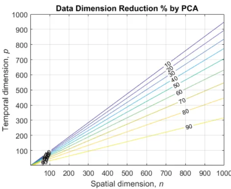
40 In this study the number of PCs from Equation (15) are selected to explain over 99.7% of the total variance in order to minimize losing information of the original data, X. In MSSA, the row length of matrix ܼ gets longer as the road network size increases, compare to SSA. Then, the dimension becomes much larger after being squared in the following step. Figure 2-2 shows the percentage of data dimension reduction by using PCA for MSSA. Compare to the case of using MSSA without PCA, for example, the data dimension in MSSA is reduced by approximately 90% by PCA if the original data dimension of ሺ݊ ൈ ݌ሻ is ሺ͵ͲͲ ൈ ͳͲͲሻ. A different number of PCs can be selected by employing information criteria, such as AIC, ICOMP, etc.

Figure 2-2 Data dimension rate of MSSA by using PCA.

The next step of MSSA is a singular value decomposition (SVD) of the squared trajectory matrix, ܥ_௒ ൌ ܻ_௖௥ܻ_௖௥். The elements of the lagged-covariance matrix ܥ௒ reflect the linear correlation between the all pair of patterns in the

(54)

41 embedding window. Thus, the recurring patterns in the time series result in a relatively high covariance in ܥ_௒ [57]. Through SVD, ܥ_௒ is decomposed into orthogonal eigenvectors as follows.

ܥ_௒ ൌ ܧȦܧ் ሺͳͻሻ

where, ܧ is the eigenvectors of ܥ௒ which are the singular vectors of ܻ௖௥, and ߉ is

a diagonal matrix that consists of ordered values, equal or greater than zero, whose square roots are the singular values of ܻ_௖௥. Then, the L largest

eigenvalues from ߉ and corresponding eigenvectors from ܧ are selected for prediction as Equation (20). In this study L=p is applied which is large enough to contain the most significant eigenvectors. Through this step, the recurring

patterns in the time series can be separate and the noise in the data can be removed [56].

ܹ ൌ ൣܧሺଵሻ_{ǡ ܧ}ሺଶሻ_{ǡ ǥ ǡ ܧ}ሺ௅ሻ_൧ _ሺʹͲሻ

Using the selected ሺܭܯ ൈ ܮሻ eigenvector matrix ܹǡthe estimation of Z is

given as the least-squares problem as follows [51, 52, 60].

ሺܼ െ ்ܹܹܼሻଶ ሺʹͳሻ

This implies that the evolution of the next vector in the trajectory matrix follows the same law of the other adjacent vectors [64].

Then, Z can be decomposed as,

ܼ ൌ ܴܲ ൅ ܳ ሺʹʹሻ

where ܲ ൌ ቂݕ_{௖௥ǡ௣ାଵ}ሺଵሻ ǡ ݕ_{௖௥ǡ௣ାଵ}ሺଶሻ ǡ ǥ ǡ ݕ_{௖௥ǡ௣ାଵ}ሺ୏ሻ ቃ். The ሺܭܯ ൈ ܭሻ and ሺܭܯ ൈ ͳሻ restriction matrices, R and Q are defined as follows.

(55)

42 ܴ ൌ ۏ ێ ێ ێ ێ ێ ۍͳ Ͳ_Ͳ _ڭ _ڮڮ Ͳ_ڭ ڭ ڭ ڭ ͳ ڮ ڭ ڮ ڭ ڭ Ͳ ڭ ڭ ڮ ڭ ڮ ͳ ڭ ڭ ڭ ڭ ڮ Ͳ ڮ ڭ ے ۑ ۑ ۑ ۑ ۑ ې ǡܳ ൌ ቂͲǡ ݕ_௖௥ǡ௣ሺଵሻǡ ǥ ǡ ݕ_{௖௥ǡ௣ିெାଶ}ሺଵሻ ǡ ǥ ǡͲǡ ݕ_௖௥ǡ௣ሺ௄ሻǡ ǥ ǡ ݕ_{௖௥ǡ௣ିெାଶ}ሺ௄ሻ ቃ் ሺʹ͵ሻ

By decomposing Equation (21) with Equation (22), the future component of the time series data can be obtained as Equation (24) [51, 52]

ܲ ൌ ሺܫ െ ்்ܴܹܹܴሻିଵ்்ܴܹܹܳ ሺʹͶሻ

where, I is a ሺܭ ൈ ܭሻ identity matrix.

Finally, the predicted speed is calculated by re-centering the values of P

and multiplying them with the eigenvectors from Equation (14).

Case Study

Data description

The proposed prediction algorithm was applied to speed data for Interstate 40 (I-40) in Tennessee from two data sources: (a) traffic detector data, named Remote Traffic Microwave Sensors (RTMS), which is collected every 30 seconds from over 1,000 traffic detector stations on interstate highways in Tennessee, and (b) probe-based link speed data, named National Performance Management

Research Data Set (NPMRDS). For RTMS, the detector stations are located only in major urban areas of the state. Therefore, 41 stations in the 21.3 mile-long westbound I-40 segment were selected, which is a major corridor in Knoxville, Tennessee. The stations are on average 0.5 miles from each other. Traffic speeds for the intermediate locations in 0.1-mile increments between two

(56)

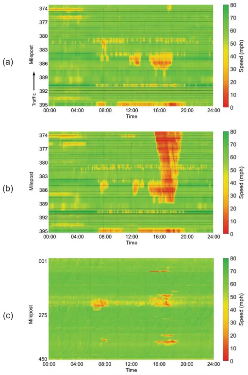
43 consecutive stations were interpolated using the adaptive smoothing method [65] in order to augment the spatial resolution of the data by 213.

The speed data from September 23 and September 30 in 2016, both of which were Fridays, were collected from the detectors and averaged in five minutes, i.e., the data dimension is ሺʹͳ͵ ൈ ʹͺͺሻ for each day. Both days were selected based on the fact that there was no incident in the first day while there was a severe incident on the second day. The incident was verified by the traffic incident data log from the local transportation management center (TMC). Since prediction of unexpected events, such as crashes, adverse weather conditions, etc., in the spatiotemporal domain is highly intractable, it is worth testing how quickly the speed prediction algorithm can adapt or how sensitive it is to sudden changes in traffic conditions.

In order to evaluate the proposed algorithm performance for a longer road segment, i.e., larger data dimension, the NPMRDS data were used. For

NPMRDS, the spatial coverage is the entire interstate highway systems in the state. In this study, the five-minute average speeds of NPMRDS for the 298 road links of a 451-mile-long I-40 westbound segment on February 3rd_{, 2017 were}

collected. Please note that five minutes are the highest resolution for the available NPMRDS dataset, i.e., the data dimension is ሺʹͻͺ ൈ ʹͺͺሻ. Figure 2-3 shows examples of the data visualizations.

Performance measures

To evaluate the prediction performance of the proposed algorithm, three error measures were used, which are the mean absolute error (MAE) and mean absolute percentage error (MAPE). They are defined as follows.

ܯܣܧ ൌ ͳ

ܰ෍ȁݔ௜ െ ݔො௜ȁ ே

௜ୀଵ

(57)

44 (a)

(b)

(c)

Figure 2-3 Speed data visualizations: (a) RTMS – September 23, 2016; (b) RTMS – September 30, 2016; and (c) NPMRDS – February 3, 2017.