Semiparametric multivariate volatility models
Christian M. Hafner
1Jeroen V.K. Rombouts
2Econometric Institute Report EI 2004-21
Abstract
Estimation of multivariate volatility models is usually carried out by quasi max-imum likelihood (QMLE), for which consistency and asymptotic normality have been proven under quite general conditions. However, there may be a substan-tial efficiency loss of QMLE if the true innovation distribution is not multinormal. We suggest a nonparametric estimation of the multivariate innovation distribution, based on consistent parameter estimates obtained by QMLE. We show that under standard regularity conditions the semiparametric efficiency bound can be attained. Without reparametrizing the conditional covariance matrix (which depends on the particular model used), adaptive estimation is not possible. However, in some cases the efficiency loss of semiparametric estimation with respect to full information maximum likelihood decreases as the dimension increases. In practice, one would like to restrict the class of possible density functions to avoid the curse of dimen-sionality. One way of doing so is to impose the constraint that the density belongs to the class of spherical distributions, for which we also derive the semiparametric efficiency bound and an estimator that attains this bound. A simulation experiment demonstrates the efficiency gain of the proposed estimator compared with QMLE.
Keywords: Multivariate volatility, GARCH, semiparametric efficiency, adaptivity. JEL Classification: C14, C22.
1Econometric Institute, Erasmus University Rotterdam, P.O.B. 1738, 3000 DR Rotterdam,
Nether-lands,[email protected]
2CORE and Department of Economics, Universit´e catholique de Louvain, Voie du Roman Pays 34,
1
Introduction
Modelling correlations of multivariate financial time series has attracted considerable in-terest recently, as computing power more and more enables the researcher to model large covariance matrices in flexible ways. For example, two quite general, nonnested classes of models are the so-called VEC GARCH model described by Engle and Kroner (1995), and the dynamic conditional correlation (DCC) model of Engle (2002), including exten-sions allowing e.g. for asymmetries analogous to the univariate GARCH literature. For a comparison and other models, see the survey by Bauwens, Laurent and Rombouts (2004). In this paper we leave the particular form of the conditional covariance matrix un-specified. All we assume is that it depends on a finite dimensional parameter vector, and the objective is to find efficient estimators of this parameter. Estimation by maximum likelihood is straightforward if one supposes a specific parametric distribution of the in-novations. However, the choice of this distribution can be quite problematic. Usually one assumes normality, which provides the so-called quasi maximum likelihood estimator (QMLE). It is now well-known that QMLE is consistent under quite general conditions, even if the true underlying distribution is not normal, see e.g. Bollerslev and Wooldridge (1992) and Jeantheau (1998). However, in the case of misspecification there may be a substantial efficiency loss of QMLE compared with the correctly specified maximum like-lihood estimator (MLE). On the other hand, assuming a non-normal distribution entails the risk of inconsistent parameter estimation if the distribution is misspecified.
In this paper we follow a nonparametric approach in letting the data determine the distribution of the innovations. With the typically large data sets in finance we would expect to obtain density estimates that are sufficiently close to the true distribution of the innovations. As our model consists of a finite dimensional parameter describing the volatility and correlation dynamics and an infinite dimensional parameter describing the innovation distribution, it may be called semiparametric (SP) as in Engle and Gonzalez-Rivera (1991), who consider univariate GARCH models.
The SP approach is typically more efficient than QMLE. The case where SP estimators are asymptotically as efficient as maximum likelihood estimators where the true distribu-tion is known is usually referred to as adaptivity. For example, in a univariate framework, adaptive estimation of ARMA models has been treated by Kreiss (1987). Often, pa-rameters describing the autoregressive dynamics of a model can be estimated adaptively, whereas scale parameters cannot. For univariate GARCH models, Linton (1993) and Drost and Klaassen (1997) show that adaptive estimators of the autoregressive parame-ters can be constructed by reparameterizing the volatility process. The same might be
possible in the multivariate case, but it will depend on the particular model. As we want this to be sufficiently general, the best we can do is to construct estimators that achieve the semiparametric lower bound. It turns out that this is possible. We show that the semiparametric lower bound is in general different from the parametric lower bound, so that adaptive estimation of the parameter vector is not possible. We characterize some selected distributions and the associated semiparametric lower bound with respect to their distance from the parametric lower bound.
To facilitate the applicability of the model, one can for example assume a priorithat the innovation distribution belongs to the class of spherical distributions. This bears the important advantage that a nonparametric estimator of the innovation distribution can be constructed in such a way that it has the univariate convergence rate. Hence, there is no ‘curse of dimensionality’ and the proposed procedure can be applied to highly dimensional systems, if sufficient structure is put on the multivariate volatility model to keep the number of parameters under control. Of course, restricting the class of distributions increases the lower bound of the semiparametric estimator, but it will remain more efficient than QMLE. In a simulation study using a multivariatetdistribution, we show that there are substantial efficiency gains of SP over QMLE.
The paper is organized as follows. First, the model framework and the traditional es-timation method is introduced. The third section discusses the nonparametric eses-timation of the innovation distribution, as well as the efficiency of SP estimators. In the fourth section a simulation study is provided. Some Lemmata used in the proofs are given in Appendix B, and the proofs of the propositions in Appendix C. For convenience we sum-marize some results of matrix algebra and calculus that are used in the paper in Appendix D.
2
The model and assumptions
Consider a vector stochastic process {εt}of dimension N with a countable index set and
an uncountable state space. We assume that εt has the properties of a conditionally
heteroskedastic error term, i.e., it has mean zero and is serially uncorrelated. We can write the basic model as
εt =Ht(θ)1/2vt, (1)
where Ht(θ) is a symmetric and positive definite matrix that may depend on past
infor-mation up to timet−1, and θ is a finite dimensional parameter vector, θ∈Θ⊂RK. As
usual, we condition on the sigma field generated by all the information (here theεt’s) until
Occasionally, we will suppress the dependence ofHt onθ for notational convenience. We
define the square root ofHtas in (62) so thatHt1/2 is also symmetric and positive definite.
In the following we make assumptions about the innovation term vt, where we denote
byIN the identity matrix of dimension N.
Assumption 1 The stochastic error {vt} is an i.i.d. sequence with E[vt] = 0, E[vtvt0] =
IN and finite fourth moments.
Because vt is independent of Ft−1, it follows that the conditional covariance matrix of εt
is Ht. Note that Assumption 1 excludes, for example, a multivariate t distribution with
4 or less degrees of freedom. The assumption of finite fourth moments of vt does not
restrict εt to have finite fourth moments. However, to prove consistency and asymptotic
normality of estimators such as QML one typically needs higher moments conditions for
εt as well. Next we make assumptions about the distribution of vt.
D = ½ g :RN →R ++| Z g(x)dx= 1, Z xg(x)dx= 0, Z xx0g(x)dx=I N,∀isup|g(i)(x)|<∞, Mψψ <∞ ¾ (2) where R++ = (0,∞), g(i)(x) denotes the ith partial derivative of g(·), and Mψψ is the
Fischer information for scale, i.e. Mψψ = E[ψtψ0t]<∞, where
ψt(vt(θ)) =−vec µ IN + ∂logg(vt) ∂vt v0 t ¶ (3) is the score vector with respect to the scale parameters.
Assumption 2 Let vt have density function g(vt)∈ D.
The assumption of a finite Fischer information for scale is standard in the literature on semiparametric scale models, see e.g., Linton (1993) and Drost and Klaassen (1997). Note that g is not required to be in a parametric class of densities, so that it can depend on a possibly infinite dimensional vector η. The vector η can be regarded as a nuisance parameter in our framework, since we are primarily interested in the estimation of θ.
Next, we summarize regularity conditions that are used by Jeantheau (1998) and Comte and Lieberman (2003) to show consistency of quasi maximum likelihood estimators.
Assumption 3 We assume the following conditions.
2. ∀θ0 ∈Θ, model (1) admits a unique strictly stationary and ergodic solution εt.
3. There exists a deterministic constant c >0 such that ∀t, ∀θ ∈Θ, |Ht(θ)| ≥c.
4. ∀θ0 ∈Θ, E[|log(|Ht(θ)|)|]<∞
5. The model is identifiable.
6. Ht(θ) is a continuous function of θ.
Several specifications have been proposed forHt, see Bauwens, Laurent and Rombouts
(2003) for a survey. Our results concerning semiparametric estimation ofθ are sufficiently general to be applicable to any such specification as long as the regularity conditions of Assumption 3 hold. However, in our simulation study of Section 4 we will work with the so–called VEC representation of a multivariate GARCH(p, q) model, which is given by
ht= vech(Ht) =ω+ q X i=1 Aivech(εt−iε0t−i) + p X j=1 Bjvech(Ht−j), (4)
where Ai and Bi are N∗ ×N∗ parameter matrices, and ω is an N∗ parameter vector
with N∗ = N(N + 1)/2. If one imposes restrictions on the parameters ω, A
i and Bj
that guarantee positive definite Ht, such as the so-called BEKK model of Engle and
Kroner (1995), then a sufficient condition for stationarity of εt is that the eigenvalues of
Pq
i=1Ai+
Pp
j=1Bj have modulus smaller than one.
We now turn to the problem of estimating θ. If one supposes that the distribution of
vt is known then maximum likelihood estimation (MLE) is in principle straightforward.
Nevertheless, because the number of parameters is often large, estimation can become a tedious exercise. Ifvtis assumed to be normally distributed with zero mean vector andIN
variance matrix then εt will be conditionally normally distributed with zero mean vector
and Ht as covariance matrix. The likelihood, up to an additive constant, for a sample of
n observations then takes the form
Lqml(θ) =− n X t=1 1 2log|Ht| − 1 2ε 0 tHt−1εt. (5) Defining lqmlt (θ) = −1
2log|Ht| − 12ε0tHt−1εt, we can write Lqml(θ) =
Pn
t=1l qml
t (θ). As
shown by Bollerslev and Wooldridge (1992) in a general conditional heteroskedasticity framework, maximizing (5) provides consistent estimates even if the likelihood is mis-specified under fairly general conditions. Therefore this method has been termed Quasi Maximum Likelihood (QML) estimation. We next assume finiteness of expectations of the Hessian and the outer product of the gradients.
Assumption 4 We assume that 1. I =E h ∂lqmlt ∂θ ∂ltqml ∂θ0 i <∞ 2. J =−E h ∂2lqml t ∂θ∂θ0 i <∞ 3. For all i, j, k, E h supkθ−θ0k≤δ ¯ ¯ ¯ ∂3lt(θ) ∂θi∂θj∂θk ¯ ¯ ¯ i <∞ for all δ >0,
where expectations are taken with respect to the true distribution and are evaluated at the true parameter vector θ0.
Under Assumptions 1 to 4, Comte and Lieberman (2003) prove that the asymptotic distribution of QML parameter estimates ˜θ is given by
√
n(˜θ−θ)−→D N(0, Vqml)
with Vqml = J−1IJ−1. In the case of correct specification, i.e., the distribution of vt
is indeed multinormal, J = I, and Vqml = I−1. Note that our Assumption 1 of vt
being i.i.d. is stronger than Comte and Lieberman’s assumption of vt being a martingale
difference sequence. For much of our paper, Assumption 1 can probably relaxed tovtbeing
a martingale difference, but we prefer to follow most of the semiparametrics literature, which usually assumes i.i.d. errors, because we rely on many results of this literature. On the other hand, Comte and Lieberman (2003) assume that the components ofvt for a
giventare independent, which seems to be a rather strong assumption. We believe that it should be possible to prove their asymptotic result without this independence assumption but leave this open to debate.
While the QML estimator is consistent, it is inefficient if the likelihood is misspecified. Therefore one sometimes considers the multivariatetdistribution as an appropriate choice because of potential fat tails in the innovations. The drawback of this assumption is that if the assumption of a specific non-normal distribution is not correct, then in general the estimator may not even be consistent, see e.g. Bollerslev and Wooldridge (1992). Therefore, we will not pursue the assumption of a specific parametric distribution in our paper. In the next section we formalize our motivation for giving all the weight to the data in search for a suitable distribution.
3
Semiparametric estimation
This section describes the methodology used to obtain semiparametric GARCH estima-tors. We consider two cases. In the first case, no assumption is made about the innovation
density besides the regularity conditions of the previous section. In the second case, we assume that the innovation density belongs to the class of spherical densities. We then describe nonparametric density estimators in the alternative cases.
3.1
Semiparametric estimation in the general case
This section describes first a simple iterative estimation procedure and then considers a more efficient semiparametric estimator.
For a general innovation density g(·), the log likelihood may be written as
L(θ) =−1/2 n X t=1 log|Ht(θ)|+ n X t=1 logg(Ht(θ)−1/2εt). (6)
Note that Assumption 1 requires that g(·) is a density with mean zero and identity covariance matrix. Without this assumption the model would not be identified. In the general case, one idea to estimate g(·) is to first use QMLE (i.e. Gaussiang(·)) to obtain standardized residuals, and then estimate the density g(·) nonparametrically. A simple estimation algorithm is the following.
1. Use QMLE to obtain a consistent estimate of θ, ˜θ, say, that gives ˜Ht=Ht(˜θ).
2. Calculate standardized residuals, ˜vt = ˜Ht−1/2εt. Make sure that they have mean
zero and variance IN.
3. Estimate nonparametrically the density g(·) of ˜vt, giving ˆg(·).
4. Maximize L keeping ˆg(·) fixed.
This procedure can be viewed as a generalization of the one suggested for univariate GARCH models by Engle and Gonzalez-Rivera (1991). For the estimation of g(·) in step 3, one can use any nonparametric estimation method. For example, we use kernel density estimators as described in Section 3.3. However, as already noticed by Engle and Gonzalez-Rivera (1991), this semiparametric estimator is not likely to achieve the semiparametric lower bound in general.
In the following we propose a semiparametric estimator that attains the semiparamet-ric lower bound and is based on well-known results of the literature on semiparametsemiparamet-ric estimation. In the context of GARCH models, standard references are Linton (1993), Drost and Klaassen (1997) and Gonzalez-Rivera and Drost (1999). A detailed description of general semiparametric estimation theory and adaptivity is beyond the scope of this
paper. We refer to Bickel (1982), Newey (1990), Steigerwald (1992) and Drost, Klaassen and Werker (1997) for details.
One can estimate the semiparametric model using a two-step procedure that uses the so-called influence function to correct an initial consistent estimator such as QML. The correction is essentially a one-step Newton-Raphson algorithm based on the score vector of the likelihood. Assume for now that the unknown densityg ofvtis parameterized by some
nuisance parameterη, and write this density asg(vt, η). A particular parametrization ofg
is known as parametric submodel. Let us write the log likelihood as L(θ) =Pnt=1lt(θ, η)
with lt(θ, η) = − 1 2log|Ht(θ)|+ logg(Ht(θ) −1/2ε t, η).
and denote by ˙lt(θ, η) = ∂lt/∂θ the score vector w.r.t. the parameter of interest, and
by st(θ, η) = ∂lt/∂η the score w.r.t. the nuisance parameter. It is easily seen that
E[st(θ, η)] = 0. Also, recall that g is restricted to be density of a mean-zero, identity
covariance matrix random vector, so that st(θ, η) has to be orthogonal to the vector
Ft = (vt,vech(vtvt0 −IN)). In the following we suppress the dependence of lt and ˙lt on η
for notational convenience.
In order to obtain efficient estimates, it is required to eliminate the variation of ˙lt(θ)
that is due to the nuisance parameter η. This is achieved by projecting the score on the so-called tangent set, which is the infinite dimensional Hilbert space spanned by all functions with the same characteristics as st(θ, η), that is, mean zero and orthogonal to
Ft. Thus, the tangent set is defined by
T ={f :RN →RK |E[f(v
t)] = 0,E[f(vt)Ft0] = 0,E[f(vt)f(vt)0]<∞}
To do the projection against T it is often crucial to factorize the score lt(θ) into a
term that only depends on the past and another that depends on the nuisance parameter. The next proposition shows that this is possible for the model under study.
Proposition 1 For the model (1), the score vector takes the form ˙ lt(θ) =Wt(θ)ψt(vt(θ)) (7) where Wt(θ) = ∂vec(Ht)0 ∂θ DND + N(IN ⊗Ht+Ht1/2⊗Ht1/2)−1 and ψt is given by (3).
Note that Wt is Ft−1-measurable and depends only on the specification of Ht(θ). The
stochastically independent. As a corollary, note also that the score vector is a martingale difference sequence, which is typically used for deriving the asymptotic distribution of the maximum likelihood estimator. The reason is that E[ ˙lt(θ) | Ft−1] = WtE[ψt | Ft−1] =
WtE[ψt] = 0 because E[ψt] = 0 as implied by Assumptions 1 and 2.
Let Mψψ = E[ψtψ0t] as in Assumption 2. Furthermore, let MψF = E[ψtFt0], MF ψ =
M0
ψF, and MF F = E[FtFt0]. We can now derive the projection of ˙lt(θ) on the tangent set.
The orthogonal complement of this projection is the so-called efficient score funtion, that can be used to do a one-step Newton-Raphson improvement of the QML estimator.
Proposition 2 The projection of l˙t(θ) on T is given by
Pt(θ) = P(˙lt(θ)| T) =E[Wt(θ)]
¡
ψt−MψFMF F−1Ft
¢
. (8)
We now propose the following efficient semiparametric estimator, ˆ θ= ˜θ+ Ã n X t=1 ˙ `∗ t(˜θ) ˙`∗ 0 t (˜θ) !−1 n X t=1 ˙ `∗ t(˜θ) (9) where ˙`∗
t(θ) = ˙`t(θ)−Pt(θ) is the efficient score function.
Under weak regularity conditions listed by Bickel (1982) and Schick (1986), see also Newey (1990), the asymptotic distribution of the estimator (9) is given by
√
n(ˆθ−θ)−→D N(0, Vsp)
with Vsp = E[ ˙`∗t`˙∗0t]−1.
By definition, adaptive estimation is possible if and only ifPt(θ) = 0, which means that
the semiparametric efficient score, ˙`∗
t, is equal to the parametric score ˙`t and, hence, Vsp
is equal to the parametric lower bound, Vml = E[ ˙`t`˙0t]−1. In the following we characterize
the asymptotic covariance matrices of the three estimation methods in terms of Wt and
ψt.
Proposition 3 Under Assumptions 1 to 4, the information matrices can be expressed as
V−1 ml = E[WtMψψWt0] (10) V−1 sp = E[WtMψψWt0]−E[Wt]QE[Wt0] (11) Vqml−1 = E[WtMψFWt0]E[WtMF FWt0]−1E[WtMF ψWt0] (12) with Q=Mψψ −MψFMF F−1MF ψ (13)
As a corollary, we obtain that the difference of the information between the MLE and the semiparametric estimator is given by the positive semi-definite matrix
V−1
ml −Vsp−1 = E[Wt]QE[Wt0].
The matrix Q determines the inefficiency of the SP estimator w.r.t. MLE. Adaptive estimation is possible if and only if Q = 0. This would clearly be a special case and we show later that in certain sub-classes of D, Q = 0 happens only if vt is Gaussian
distributed. The conclusion is that adaptive estimation of the model in (1) without reparameterization of Ht is not possible. Similar to Gonzalez-Rivera and Drost (1999)
it can also be verified that V−1
sp − Vqml−1 is positive semi-definite, meaning that the SP
estimator is at least as efficient as the QML estimator.
In practice, the moment matrix MF F can be replaced by its empirical counterpart
using the empirical moments of the standardized residuals ˜vt obtained after the first
step. That is, having a consistent estimate ˜θ, one can construct standardized residuals ˜
vt =Ht(˜θ)−1/2εt. Defining further Fbt = (˜vt,vech(˜vtv˜0t−IN)), a consistent estimator MF F
is given byMcF F =n−1
Pn
t=1FbtFbt0. The matrixMψF does not need to be estimated as the
following proposition shows, because an expression is available that holds for any g ∈ D. To calculate Pt(˜θ) in (8), one still needs to estimate ˙`t(˜θ) and ψt(˜θ) which both depend
on the unknown innovation density g, for which nonparametric methods such as those outlined in Section 3.3 are available.
To characterize the distance of the SP estimator from adaptivity, it will be necessary to evaluate the matrices Mψψ and MF F by numerical integration. However, there are
special cases where they take simple forms. In the following we consider two sub-classes of D for which calculation turns out to be particularly simple. The first one is the class of spherical distributions: Ds = © g :RN →R ++|g ∈ D,∃f :g(x) =f(x0x) ª (14) and the second one is the class where the components are independent with identical and symmetric marginal densities:
Di = ( g :RN →R ++ |g ∈ D, g(x) = N Y i=1 h(xi), h(xi) =h(−xi) ) , (15) where h(·) is the marginal density of any component of vt.
The following discussion analyzes the properties of the SP estimator w.r.t. MLE in the case that g happens to be in Ds or in Di without having made this assumption to
construct the estimator. The situation where one has superior knowledge about g and, for example, knows a priori that g is in Ds, is different and is treated in Section 3.2.
The matrix MF F depends on the structure of fourth moments of vt. Lemma 6 implies
that, for spherical distributions, the marginal kurtosis κ = E[v4
ti] is linked to any
co-kurtosis c=E[v2
tiv2tj], j 6=iby κ= 3c, and MF F depends on only one parameter.
Proposition 4 1. If g ∈ D, then MψF = h 0N2×N 2DNDN+D+N0 i 2. If g ∈ Ds, then MF F = " IN 0N×N∗ 0N∗×N 2cDN+DN+0+ (c−1)vech(IN)vech(IN)0 # (16) Mψψ = 2τ DNDN++ (τ−1)vec(IN)vec(IN)0 (17) where τ =E "µ ∂logg(x) ∂x1 ¶2 x21 # /3. (18) 3. If g ∈ Di, then MF F = " IN 0N×N∗ 0N∗×N IN∗+ [IN∗¯ {(κ−2)vech(IN)vech(IN)0}] # (19) Mψψ = τ2DNDN0 +DN[IN∗¯ {(τ1−1−τ2)vech(IN)vech(IN)0}]D0N (20) where τ1 = 3τ, ¯ is the Hadamard product (elementwise multiplication), κ is the
marginal kurtosis, and
τ2 =E "µ ∂logg(x) ∂x1 ¶2# . (21)
Note that Assumption 2 implies thatτ in (17) andτ2 in (20) are finite. The scalar τ2 can
be interpreted as the Fischer information for location which for distributions in Di is the
same for all components.
For illustration consider the bivariate case (N = 2). From Proposition 4 it follows immediately that, for g ∈ Ds,
Q=DN 3τ −1− 3c−1 c(2c−1) 0 τ−1− c(2c1−−c1) 0 τ− 1 c 0 τ −1− 1−c c(2c−1) 0 3τ −1− c(2c3c−−11) DN0 , and for g ∈ Di, Q=DN τ1−κ−41 0 0 0 τ2−1 0 0 0 τ1− κ−41 D0 N.
Clearly, the parametric and semiparametric lower bounds coincide in the Gaussian case since then c= 1, τ = 1 and therefore Q= 0. Whether there are other distributions for which this happens is our next concern. In a univariate framework, Gonzalez-Rivera (1997) has shown that a class of symmetric bimodal distributions allows to attain the parametric lower bound, and for N = 1 this distribution is in Di. The following
propo-sition states that, for higher dimensions, the Gaussian distribution is the only one in Di
and in Ds for which parametric efficiency can be attained. We do not search here for
other, possibly asymmetric, distributions for which the two bounds coincide. It may be possible that such distributions exist, but we leave this as a topic for further research.
Proposition 5 For the estimation of model (1), the multinormal distribution is the only one in Ds for which the parametric and semiparametric lower bounds coincide. If N >1,
then it is also the only distribution in Di for which this occurs.
Let us now look at three examples of distributions in Ds and at two examples of
distributions in Di. Table 1 reports the spectral norm of Qfor these distributions, which
for the case of real, positive semi-definite matrices is equal to the spectral radius ρ(Q), i.e., the largest eigenvalue.
1. The density of a symmetric standardized multivariate t distribution is given by
g(vt) = Γ¡ν+N 2 ¢ {π(ν−2)}N/2Γ(ν/2) µ 1 + v 0 tvt ν−2 ¶−(ν+N)/2 (22) where Γ(p) = R0∞xp−1e−xdxis the gamma function. To ensure finite fourth moments
of vt we will assume in the following that ν >4. Under the density given in (22),
c = (ν −2)/(ν −4) and τ = (ν+N)/(ν +N + 2). Note that for ν −→ ∞, since the limiting distribution is a Gaussian, c = 1, τ = 1, and Mψψ = MψF = MF F =
2D+
ND+N0. For increasing dimensions N, τ converges to 1 and Mψψ converges to
2D+ ND+N0.
2. The second example is a multivariate Laplace distribution with density
g(vt) = (N + 1)N/2Γ(N/2) 2πN/2(N −1)! exp(− p (N + 1)v0 tvt) (23)
For N = 1,2,3 we find c= (N + 3)/(N + 1) and τ = (N + 1)/(N + 2). Although we do not use it here, we conjecture that these formulae forcandτ hold for any N, which would imply that c→1 and τ →1 forN → ∞, which in turn implies using Proposition 4 that the multivariate Laplace density converges to a multinormal distribution with increasing dimension.
3. The third example is an elliptically symmetric (ES) multivariate logistic distribution with density
g(vt) =c1
e−c2v0tvt
(1 +e−c2v0tvt)2 (24)
with constants c1 and c2 such that (24) integrates to one and Var(vit) = 1. We
calculate the valuesc1, c2, the co-kurtosis C, andτ by numerical integration. Note
that the univariate distribution (N = 1) is different from the distribution usually called logistic. For example, the distribution in (24) is platykurtic, whereas the standard logistic is leptokurtic. The ES logistic distribution is mentioned by Jensen (1985).
4. A product of standardized logistics:
g(vt) = 3N/2 πN N Y i=1 e−vit (1 +e−vit)2 (25)
In the univariate case, Q = τ1−1−4/(κ−1) = 0.18. We find that this value is
larger than τ2 −1 ≈ 0.10, so that the largest eigenvalue remains 0.18 for higher
dimensions. 5. A product of bimodals: g(vt) = µ λ 2 ¶N λ/2 Γ(λ/2)−N N Y i=1 |vit|λ−1e− λ 2v2it, (26)
where either λ = 1 (the multinormal case) or λ > 2 to ensure continuity and differentiability. ForN = 1, this density has been shown by Gonzalez-Rivera (1997) to giveQ= 0. Table 1 reports the value of ρ(Q) for the case λ= 3.
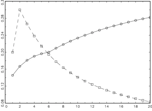
Note that the densities in (22), (23) and (24) are spherical and those in (25) and (26) are in Di. Note also that the results reported in Table 1 generalize those for the case
N = 1 listed by Gonzalez-Rivera (1997). In the univariate case, Q is a positive scalar, so that ρ(Q) is just this scalar itself. Figure 1 displays ρ(Q), viewed as a function of the dimension N, for the Laplace and the t12 distribution. We noticed that, for the tν
distribution, there is a break at N = ν−6, ν ≥ 7, in the sense that ρ(Q) is concave for
N ≤ν−6 and forN ≥ν−6, but not for all N ≥1. We did not try to prove this result but found it curious enough to mention.
3.2
Semiparametric estimation in
D
sThe preceding discussion has not imposed any restriction on the density of vt other than
conditions. Nonparametric estimators of this density will therefore have to be of full generality and have to ensure consistency for any such density. It is well known that nonparametric estimation in high dimensions suffers from the so-called curse of dimen-sionality, that is, the data sparseness problem described by Silverman (1986). In high dimensions, convergence rates become very slow and the number of observations required to obtain reasonable estimates goes beyond what is typically available in economics, even in finance.
One way to impose more structure ongthat solves the dimensionality problem but still leaves sufficient flexibility is to assume thatgbelongs to the class of spherical distributions, which we do in the following.
Assumption 5 For the density g, assume g ∈ Ds, where Ds is defined by (14).
The density g(vt) is said to be spherical if there exists a positive function f such that
g(vt) = f(wt) with wt = vt0vt. Examples of spherical distributions are the multivariate
versions of the normal, the t and Laplace distributions. The relevance of these distribu-tions for empirical work arises from the fact that one often observes fat tails in empirical data, even after correcting for time-varying volatility. They exclude skewness, but in finance this has been of minor interest compared with the leptokurtosis effect. The theo-retical relevance of Assumption 5 lies in the fact that the class of spherical distributions (or elliptical, respectively, if the conditional distribution of εt is considered) is the most
general one that is consistent with the conditional capital asset pricing model, as shown by Berk (1997), see also Hodgson and Vorkink (2003). In our framework, the main advan-tage of Assumption 5 is that it allows for univariate convergence rates of nonparametric estimators of g.
Proposition 6 Under Assumption 5, the score vector is given by (7) whereWtsimplifies
to Wt(θ) = ∂vec(Ht)0 ∂θ (H −1/2 t ⊗Ht−1/2) and ψt is given by (3).
Semiparametric estimators of model (1) that are based on Assumption 5 have a lower bound that is larger than the bound in the general case. The score in the nonparametric direction, s(θ, η), is now a function of vt only through wt, and therefore, the tangent
set contains functions that all depend on wt only. But still, these functions have to be
orthogonal toFtbecauseg is restricted to have mean zero and identity covariance matrix.
Thus, the tangent set under Assumption 5 is defined by
Note also that Ts ⊂ T. We can now derive the projection of ˙lt(θ) on Ts.
Proposition 7 Under Assumption 5, the projection of l˙t(θ) on Ts is given by
St(θ) = P(˙lt(θ)| Ts) =E[Wt(θ)] ³ ˜ ψt−MψF˜ MF F−˜1F˜t ´ , (27) where ψ˜t=E[ψt|wt], F˜t=E[Ft |wt], MψF˜ =E[ ˜ψtFt0] and MF F˜ =E[ ˜FtFt0]
The efficient semiparametric estimator is given by (9) where ˙`∗
t(θ) is replaced by ˙`∗t(θ) =
˙
`t(θ)−St(θ).
Note that ˜Ftcontains the conditional expectations E[vt |wt] and E [vtv0t|wt]. The first
one is zero since for any given wt, the distribution of vt conditional on wt is symmetric
in vt. For the second conditional expectation, E [vtv0t|wt], Hodgson and Vorkink (2003)
describe a simple estimation algorithm after the first estimation step.
Under sphericity, estimation of ˜ψt reduces to the estimation ˜Ft by noting that there
exists a function f such that g(vt) =f(wt) and
E · ∂logg(vt) ∂vt v0 t ¯ ¯ ¯ ¯wt ¸ = E · 2f(wt)−1 ∂f(wt) ∂wt vtv0t ¯ ¯ ¯ ¯wt ¸ = 2f(wt)−1 ∂f(wt) ∂wt E [vtvt0 |wt]
Another restriction of D that may be interesting for practical work is to assume that
g ∈ Di, where Di is given in (15). One would again obtain univariate convergence rates
and avoid the curse of dimensionality. Another advantage is that under componentwise independence of vt it is possible to define impulse response functions for volatility that
avoid typical orthogonalization and ordering problems, as shown by Hafner and Herwartz (2004). It is also obvious that Proposition 6 holds under the assumptiong ∈ Di. However,
we have not further investigated efficient semiparametric estimation in this class but leave it to future research.
3.3
Nonparametric density estimation
For the nonparametric density estimation, we use kernel estimates. A general multivariate kernel density estimator with bandwidth matrix H and multivariate kernel K can be written as ˆ gH(x) = 1 n|H| n X t=1 K(H−1(vt−x))
Since the scale of the variables should be the same (same variance in all directions), it is reasonable to use a scalar bandwidth, H = hIN, with h > 0. It is well known that
by requiring nhN → ∞ and h→ 0 as n → ∞, the multivariate kernel density estimates
bandwidth isn−1/(4+N). We use here a rule of thumb bandwidth as proposed by Silverman
(1986). Furthermore, we use a product kernel K(x) = QNi=1K(xi) and some univariate
kernel functionK such as Gaussian, quartic or Epanechnikov. Thus, our density estimate becomes ˆ gh(x) = 1 nhN n X t=1 N Y i=1 K(vi,t −xi h )
For details on multivariate kernel density estimation see the excellent survey of Scott (1992).
The multivariate density estimation becomes difficult for high dimenensional cases. When
g(x) is spherical then its density must be of the formf(x0x) for some nonnegative function
f(·). Fang, Kotz and Ng (1990, p. 36), show that in this case the density of y =x0x can
be written as
h(y) = π
N/2
Γ(N/2)y
N/2−1f(y). (28)
Thus one can obtain an estimator of g(·) by estimating h(·) and transforming according to (28).
Since y has a positive support, one faces the problem of estimating its density near the boundary. To solve this problem, Hodgson, Linton and Vorkink (2002) and Hodgson and Vorkink (2003) apply a Box-Cox transformation to y and then use the standard kernel density estimator to the transformed variable. We use an alternative method by applying a gamma kernel estimator, see Chen (2000) who shows that gamma kernels are particularly suited for the estimation of density functions which have bounded support. The gamma kernel estimator can be written as
ˆ h(y) = 1 n n X t=1 Gρb(y),b(yt) (29)
where Gp,q is the density function of a Gamma(p, q) random variable, and
ρb(y) = ( y/b if y ≥2b 1 4(y/b)2+ 1 if y ∈[0,2b). (30) Chen (2000) also provides formula for the bandwidthbthat minimize the mean integrated squared error which we will use in our simulation study.
4
Finite sample performance
In this section we are interested in the performance of the proposed SP estimator (9) relative to the QML and ML estimator in finite samples. Intuitively, the semiparametric
method should perform better than QML, but worse than ML, when there are strong departures from normality.
For convenience we consider the VEC model in (4) of order p =q = 1. To calculate
Wt(θ) in (7) one needs to evaluate ∂vec(Ht)
0
∂θ . Deriving with respect to the parameters in
ω, Aand B we get ∂ht ∂ω0 = (IN∗−B) −1 ∂ht ∂vec(A)0 = η 0 t−1⊗IN∗+B ∂ht−1 ∂vec(A)0 ∂ht ∂vec(B)0 = h 0 t−1⊗IN∗+B ∂ht−1 ∂vec(B)0
where ηt−1 = vech(εt−1ε0t−1). The bivariate data generating process is given by
ht = 1 0.7 1 + 0.2 0 0 0 0.1 0 0 0 0.2 ε2 1,t−1 ε1,t−1ε2,t−1 ε2 2,t−1 + 0.5 0 0 0 0.1 0 0 0 0.6 h11,t−1 h12,t−1 h22,t−1 .
For the distributional assumption on vt we take the bivariate t distribution, that is
vt ∼ tν with density given in (22). In this exercise we take ν = 5. We assume that it
is known thatg belongs to the spherical class. For the nonparametric estimation of g(·), this assumption allows us to use the Gamma kernel estimator as explained in Section 3.3. The employed estimator is thus given by (9) where ˙`∗
t(θ) = ˙`t(θ)−St(θ) andSt(θ) is given
by (27). The results are displayed in Table 2.
Concerning the bias, the three estimation procedures perform similarly, perhaps one could notice that SP performs better than QML for most of the parameters. There are, however, substantial differences between the standard deviations. Clearly ML performs best for all the parameters. SP is as expected in between the two other procedures, also for all the parameters. The same holds true for the MSE of ˆθ. One can see that a good part of the loss of the inefficient QML (compared to ML) is recaptured by SP. We also compared the performance of the univariate gamma kernel estimator with the bivariate product kernel estimator when the assumption of sphericity is dropped and the projection Pt(θ) in (8) is used to construct the estimator (9). The latter estimator had
higher MSE’s for all parameters, but still considerably less than the QML mean squared errors. However, the relative performance of the multivariate kernel estimator for N >2 is likely to become worse if the dimension increases and if the true density is close to the spherical class.
5
Conclusions and outlook
This paper shows that efficiency gains of semiparametric univariate volatility models over QMLE carry over to the multivariate case. We suggest two alternative types of semi-parametric estimators. The first one applies to general innovation densities whereas the second one is based on the assumption of sphericity. A practical advantage of the spheric-ity assumption is that a nonparametric densspheric-ity estimator can be constructed that has one-dimensional convergence rate. Thus it does not run into the ‘curse of dimensional-ity’ problem. Both estimators are efficient but the semiparametric and parametric lower bounds are different in general, so that adaptive estimation is not possible. A guideline for future research may be to find, for particular model specifications, reparameteriza-tions of the conditional covariance matrix such that adaptive estimation of a subset of the parameters is possible, analogous to the univariate case. In this paper, this was not our main concern as we wanted to leave the parametric part of the model unspecified as much as possible, because a multitude of possible specifications have been proposed recently. We think that a main drawback of the general approach outlined in Section 3.1 is that, in practice, it will only be feasible in small dimensions. With the typically high dimensions encountered in finance, for example, this is certainly not a nice feature. In high dimensions one would like to reduce the dimensionality and the assumption of sphericity is only one way of doing this. Another one would be to assume that innova-tions are componentwise i.i.d., a case that we have not looked at further. There are still other ways to restrict the class of distributions to facilitate the problem of nonparametric estimation in high dimensions, and we leave this also as a topic for further research.
Finally, it may be possible to relax the assumption of an i.i.d. innovation term to, say, a martingale difference term, but proofs become considerably more complicated already in the univariate case, and one would need to control the possible temporal dependence by making further assumptions.
Acknowledgements
The authors would like to thank Luc Bauwens, Geert Dhaene, Feico Drost, Wolfgang H¨ardle, Jens Peter Kreiss, and Bas Werker for helpful discussions. We also thank partic-ipants of the CORE econometrics seminar, the York annual meeting in econometrics, the annual econometric study group meeting 2002 in Bristol, and the 2003 workshop ‘The art of semiparametrics’ in Berlin for valuable comments.
References
[1] Bauwens, L., S. Laurent & J.V.K. Rombouts (2004) Multivariate GARCH models: A survey. CORE, Universit´e catholique de Louvain, Louvain-la-Neuve, Belgium.
[2] Berk, J. (1997) Necessary conditions for the CAPM. Journal of Economic Theory73, 245–257.
[3] Bickel, P.J. (1982) On adaptive estimation. Annals of Statistics 10, 647-671.
[4] Bickel, P.J., C.A.J. Klaassen, Y. Ritov & J.A. Wellner (1993) Efficient and Adap-tive Statistical Inference for Semiparametric Models. John Hopkins University Press, Baltimore, MD.
[5] Bollerslev, T. & J. Wooldridge (1992) Quasi maximum likelihood estimation and infer-ence in dynamic models with time varying covariances. Econometric Reviews 11 ,143-72.
[6] Box, G.E.P. & J.S. Hunter (1957) Multi-factor experimental designs for exploring response surfaces. Annals of Mathematical Statistics 28, 195–241.
[7] Chen, S.X. (2000) Probability density function estimation using Gamma kernels. An-nals of the Institute of Statistical Mathematics 52, 471–480.
[8] Comte, F. & O. Lieberman (2003) Asymptotic theory for multivariate GARCH pro-cesses. Journal of Multivariate Analysis 84, 61-84.
[9] Drost, F.C., C.A.J. Klaassen & B.J.M. Werker (1997) Adaptive estimation in time series models. Annals of Statistics 25, 786-817.
[10] Drost, C.D. & C.A.J. Klaassen (1997) Efficient estimation in semiparametric GARCH models. Journal of Econometrics 81, 193-221.
[11] Engle, R.F. (2002) Dynamic conditional correlation - A simple class of multivariate GARCH models. Journal of Business and Economic Statistics 20, 339–350.
[12] Engle, R. & K. Kroner (1995) Multivariate simultaneous GARCH.Econometric The-ory 11, 122-150.
[13] Engle, R. & Gonzalez-Rivera, G. (1991), Semiparametric ARCH models. Journal of Business and Economic Statistics 9, 345-359.
[14] Fang, K.T., S. Kotz & K.W. Ng (1990) Symmetric Multivariate and Related Distri-butions. Chapman and Hall: London.
[15] Gonzalez-Rivera, G. (1997) A note on adaptation in ARCH models. Econometric Reviews 16, 55-68.
[16] Gonzalez-Rivera, G. & C.D. Drost (1999) Efficiency comparisons of maximum-likelihood-based estimators in GARCH models. Journal of Econometrics 93, 93-111. [17] Hafner, C.M. & H. Herwartz (2004) Volatility impulse response functions for
mul-tivariate GARCH models: An exchange rate illustration. Journal of International Money and Finance, forthcoming.
[18] Hodgson, D.J. & K.P. Vorkink (2003) Efficient estimation of conditional asset-pricing models. Journal of Business and Economic Statistics 52, 471-480.
[19] Hodgson, D.J., O. Linton & K.P. Vorkink (2002) Testing the capital asset pricing model efficiently under elliptical symmetry: A semiparametric approach. Journal of Applied Econometrics 17, 617-639.
[20] Jeantheau, T. (1998) Strong consistency of estimators for multivariate ARCH models. Econometric Theory 14, 70-86.
[21] Jensen, D.R. (1985) Multivariate Distributions. In Kotz, S., N.L. Johnson & C.B. Read (ed.) Encyclopedia of Statistical Sciences, 6, Wiley, pp. 43-55.
[22] Linton, O. (1993) Adaptive estimation of ARCH models. Econometric Theory 9, 539-569.
[23] Kreiss, J.P. (1987) On adaptive estimation in stationary ARMA processes. The An-nals of Statistics 15, 112-133.
[24] L¨utkepohl, H. (1996) Handbook of Matrices. New York: Wiley.
[25] Magnus, J.R. (1988) Linear Structures. London: Griffin.
[26] Newey, W.K. (1990) Semiparametric efficiency bounds. Journal of Applied Econo-metrics 5, 99-135.
[27] Schick, A. (1986) On asymptotically efficient estimation in semiparametric models. Annals of Statistics 14, 1139-1151.
[28] Scott, D. (1992) Multivariate Density Estimation : Theory, Practice, and Visualisa-tion. New York: Wiley.
[29] Silverman, B.W. (1986) Density Estimation for Statistics and Data Analysis. Chap-man and Hall: London.
[30] Steigerwald, D.G. (1992) Adaptive estimation in time series regression models. Jour-nal of Econometrics 54, 251-275.
Appendix A: Index Set Definitions
Define the index
kN
ij =i+ (j −1)(N −
j
2) (31)
and the index sets
KijN = ( ∅ N = 1 {kN ij |j = 1, . . . , N −1; i=j+ 1, . . . , N} N ≥2 (32) and KN ii ={kNii |i= 1, . . . , N} (33) The indexkN
ij is the position of the (i, j)-th element of an (N×N) symmmetric matrixA
in the vector vech(A). Remember that vech(A) containsN∗ =N(N+ 1)/2 elements. KN ij
contains all indices of the elements below the diagonal ofA in the vector vech(A), this set containsN(N−1)/2 elements. The setKN
ii contains all indices of theN diagonal elements.
For example, for N = 2, K2
ij = {2} and K2ii ={1,3}, and for N = 3, K3ij = {2,3,5} and
K3
ii={1,4,6}. Note that KijN ∪ KiiN ={1, . . . , N∗}and KNij ∩ KNii =∅.
Appendix B: Lemmata
Lemma 1 For given nonsingular matrices A, B(m×m), let Z =B⊗A+A⊗B. Then
DmD+mZ−1DmD+m =DmD+mZ−1 (34)
Proof: Assume the contrary. Then, multiplying both sides of (34) from the right by Z
gives DmD+mZ−1DmDm+Z 6= DmD+m. Using (72), one can write the left hand side of this
inequality as DmDm+Z−1ZDmD+m =DmD+mDmDm+ =DmD+m, making use of the fact that
D+
mDm =Im(m+1)/2. But this yields a contradiction, so that the original equality in (34)
must hold. ¤
Lemma 2 For given matrices A, B(m×m),
D0 m(A⊗B)DmDm+ = 1 2D 0 m(A⊗B+B⊗A) (35)
Proof: Assume the contrary. Vectorizing the left hand side of (35), one obtains (DmD+m⊗
D0
m)vec(A⊗ B). Using (67) and vectorizing the right hand side of (35), one obtains 1
2(Im2⊗Dm0 +Cmm⊗D0mCmm)vec(A⊗B). But using (70), this is equal to 12(Im2 ⊗Dm0 +
Cmm⊗D0m)vec(A⊗B) = 12[(Im2 +Cmm)⊗Dm0 ]vec(A⊗B). Finally, using (69), this is
equal to (DmDm+ ⊗Dm0 )vec(A⊗B), which yields to a contradiction. Therefore, equality
Lemma 3 For a given symmetric, positive definite matrix A(m×m),
2DmD+m(Im⊗A+A1/2⊗A1/2)−1vec(Im) = vec(A−1). (36)
Proof: Assume the contrary. The left hand side of (36) can be written as
2DmD+m £ (Im⊗A1/2)(Im⊗A1/2+A1/2⊗Im) ¤−1 vec(Im) or, using (63), as 2DmD+m(Im⊗A1/2+A1/2⊗Im)−1(Im⊗A−1/2)vec(Im).
Applying Lemma 1, this is equivalent to
2(Im⊗A1/2+A1/2⊗Im)−1DmDm+(Im⊗A−1/2)vec(Im).
As we assumed inequality in (36), we have that
2DmD+m(Im⊗A−1/2)vec(Im)= (6 Im⊗A1/2 +A1/2⊗Im)vec(A−1).
or, using (59),DmDm+vec(A−1/2)6= vec(A−1/2).However, sinceA−1/2is symmetric because
of our definition of a matrix square root in (62), it holds that vec(A−1/2) = D
mvech(A−1/2),
and because D+
mDm =Im(m+1)/2 this inequality leads to a contradiction, so that equality
must hold in (36). Q.E.D.
Lemma 4 The matrix D+
NDN+0 is a (N∗ × N∗) diagonal matrix with 1 at the (i, i)-th
position, i∈ KN
ii, and 1/2 at the (j, j)-th position, j ∈ KNij, where KijN is defined in (32)
and KN
ii in (33).
Proof: The statement holds forD+
1D1+0 = 1. Noting thatkiiN+1 =kiN−1,i−1+N+1, wherekNij
is defined in (31), and using the recursive equation for D+
N+1DN+0+1 in (74), the statement
follows by induction. Q.E.D.
Lemma 5 The matrix vech(IN)vech(IN)0 is a (N∗ ×N∗) matrix with 1 at the (i, j)-th
position, i, j ∈ KN
ii, and 0 elsewhere, where KiiN is defined in (33).
Proof: By definition, KN
ii contains the positions of the diagonal elements of a (N ×N)
matrix A in the vector vech(A). Therefore, KN
ii contains the positions of the ones in
the vector vech(IN). The matrix vech(IN)vech(IN)0 then contains ones at pairs of any
permutations of these positions, and zeros elsewhere. So there is a total ofN2 ones in the
Lemma 6 For any spherical distribution, E " N Y j=1 Xαj j # = (
0 if one (or more) αj is odd
Kα
QN
j=1 αj!
(αj/2)! if all αj are even
where α=PNj=1αj and Kα depends on α only.
Proof: see Box and Hunter (1957).
Appendix C: Proofs
Proof of Proposition 1:
Let us write the likelihood as L(θ) = Pnt=1lt(θ) with
lt=−
1
2log|Ht|+ logg(H
−1/2 t εt).
The score vector is given by
∂lt(θ) ∂θ =− 1 2 ∂log|Ht| ∂θ + ∂logg(Ht−1/2εt) ∂θ
where the first term has components
∂log|Ht| ∂θi = vec(Ht−1)0∂vec(Ht) ∂θi = Tr µ Ht−1∂Ht ∂θi ¶ = Tr µ Ht−1/2∂Ht ∂θi Ht−1/2 
using (80). With the chain rule for matrix differentiation (75), we can write
∂logg(Ht−1/2εt) ∂θi = ∂logg(x) ∂x0 ∂(Ht−1/2εt) ∂vec(Ht)0 ∂vec(Ht) ∂θi
Applying (77) and (79) we can further write
∂(Ht−1/2εt) ∂vec(Ht)0 =−(ε0t⊗IN)(Ht−1/2⊗H −1/2 t ) ∂vec(Ht1/2) ∂vec(Ht)0 (37) Then, ∂vec(Ht1/2)
∂vec(Ht)0 can be appropriately defined by noting thatHt is symmetric and by the
definition of the matrix square root (62)Ht1/2 is symmetric as well. By (78) we know that in this case ∂vech(Ht) ∂vech(Ht1/2)0 = D + N(H 1/2 t ⊗IN +IN ⊗Ht1/2)DN (38) = D+ NZDN (39)
with Z = (Ht1/2⊗IN +IN⊗Ht1/2), where D+N denotes the generalized inverse (64) of the
duplication matrixDN. If the matrixZ is invertible, a natural definition for the derivative
of the matrix square root is
∂vech(Ht1/2)
∂vech(Ht)0
= (DN+ZDN)−1 (40)
= D+
NZ−1DN, (41)
where (41) uses (73). Using (76) we then obtain
∂vec(Ht1/2)
∂vec(Ht)0
= DNDN+Z−1DNDN+ (42)
= DNDN+Z−1 (43)
by Lemma 1.
Plugging (43) into (37), we obtain
∂(Ht−1/2εt) ∂vec(Ht)0 = −(ε0 t⊗IN)(Ht−1/2⊗Ht−1/2)DND+NZ−1 (44) = −(v0 t⊗IN)(Ht1/2⊗IN)(Ht−1/2⊗Ht−1/2)Z−1DND+N (45) = −(vt0⊗IN)(IN ⊗Ht−1/2)Z−1DND+N (46) = −(v0 t⊗IN){Z(IN ⊗Ht1/2)}−1DND+N (47) = −(v0 t⊗IN)(IN ⊗Ht+Ht1/2⊗Ht1/2)−1DND+N (48)
where (45) uses the fact that both Z−1 and D
NDN+ are symmetric and (47) uses (63).
Thus, ∂logg(vt) ∂θi = −∂logg(vt) ∂v0 t (v0 t⊗IN)(IN ⊗Ht+Ht1/2⊗Ht1/2)−1DNDN+ ∂vec(Ht) ∂θi = −vec µ ∂logg(vt) ∂vt vt0 ¶0 (IN ⊗Ht+Ht1/2⊗H 1/2 t )−1DND+N ∂vec(Ht) ∂θi = −vec µ ∂logg(vt) ∂vt v0 t ¶0 W0 t withWt= ∂vec(Ht) 0
∂θ DND+N(IN⊗Ht+Ht1/2⊗Ht1/2)−1. Definingψt=−vec(IN+(∂logg(vt)/∂vt)v0t),
this can be written as
∂logg(vt)
∂θi
=ψ0
tWt0 + vec(IN)0Wt0.
However, by Lemma 3 the term vec(IN)0Wt0 is equal to 12vec(Ht−1)0∂vec∂θ(H0 t). Thus, the score vector can be written as
∂lt(θ) ∂θ = ∂vec(Ht)0 ∂θ ½ −1 2vec(H −1 t )−DNDN+(IN ⊗Ht+Ht1/2⊗Ht1/2)−1vec µ ∂logg(vt) ∂vt v0 t ¶¾
= −1 2 ∂vec(Ht)0 ∂θ vec(H −1 t ) +Wtψt+ 1 2 ∂vec(Ht)0 ∂θ vec(H −1 t ) = Wtψt, as stated. Q.E.D. Proof of Proposition 2
First note that Pt ∈ T because E[Pt] = 0, E[PtFt0] = 0, and E[PtPt0] is finite since
E[ψtψt0]<∞by Assumption 2 and E[FtFt0]<∞by Assumption 1 (finite fourth moments).
Next, we show that the orthogonal complement of the projection is orthogonal to T. It can be written as
˙
`∗t(θ) = ˙`t(θ)−Pt = (Wt−E[Wt])ψt+ E[Wt]MψFMF F−1Ft (49)
The first term on the right hand side of (49) is orthogonal to T since (Wt−E[Wt]) has
mean zero and is independent of vt and, hence, independent of all elements in T. The
second term on the right hand side of (49) is orthogonal to T because it consists of linear combinations of Ft and Ft is, by definition, orthogonal to T. Q.E.D.
Proof of Proposition 3 1. V−1 ml = E[˙ltl˙t0] = E[Wtψtψt0Wt0] = E[WtMψψWt0] 2. V−1 sp = E[˙ltl˙0t]−E[˙ltPt0]−E[Ptl˙0t] + E[PtPt0].
The second term is
E[˙ltPt0] = E £ Wtψt(ψt0 −Ft0MF F−1MF ψ)E(Wt0) ¤ = E[Wt]E[ψtψ0t−ψtFt0MF F−1MF ψ]E[Wt0] = E[Wt] ¡ Mψψ−MψFMF F−1MF ψ ¢ E[W0 t]
Similar calculations show that E[˙ltPt0] = E[Ptl˙0t] = E[PtPt0], which then gives the
stated result.
3. Recall that Vqml =J−1IJ−1, and thusVqml−1 =J I−1J with
J =−E " ∂2lqml t ∂θ∂θ0 # , I = E " ∂lqmlt ∂θ ∂ltqml ∂θ0 # , and ∂lqmlt ∂θ =WtKNFt, whereKN = h 0N2×N DN i . We have I = E[WtKNFtFt0KN0 Wt0] = E[WtKNMF FKN0 Wt0]
and J = − Z IRN g(x)∂2l qml t ∂θ∂θ0dx= Z IRN ∂g(x) ∂θ ∂ltqml ∂θ0 dx (50) = Z IRN g(x)∂logg(x) ∂θ ∂lqmlt ∂θ0 dx= E " ∂logg(x) ∂θ ∂lqmlt ∂θ0 # (51) = E [WtψtFtKN0 Wt0] = E [WtMψFKN0 Wt0] (52) Q.E.D. Proof of Proposition 4
1. MψF: Note first thatψtis orthogonal tovt: E[ψtvt0] =−E[vec{(∂logg(vt)/∂vt)vt0}vt0]
and writing this expectation elementwise one obtains −RIRN(∂g(vt)/∂vit)vjtvktdvt.
Using integration by parts, for i = j = k this is just equal to 2E[vit] = 0, and for
i=j 6=k it is equal to E[vkt] = 0, and the same holds for i=6 j 6=k and i6=j =k.
Hence, the left block of MψF is equal to 0N2×N. The right block can be written as
−E[vec(∂logg(vt)
∂vt
v0
t)vech(vtv0t)0]−vec(IN)vech(IN)0. (53)
Writing the expectation term in (53) elementwise, one obtains−RIRN
∂g(vt)
∂vit vjtvktvltdvt
which for i = j = k = l is equal to 3, for i = j 6= k = l is equal to 1, and zero otherwise. Therefore, we have the following symmetry relation,
Z IRN ∂g(vt) ∂vit vjtvktvltdvt = Z IRN ∂g(vt) ∂vjt vitvktvltdvt,
and, as a consequence, the first term in (53) can be written as DNJt where
Jt =−E · vech µ ∂logg vt vt0 ¶ vech(vtv0t)0 ¸
is, due to the above elementwise calculations, a (N∗ ×N∗) matrix with 3 at the
(i, i)th position, i ∈ KN
ii; a 1 at the positions (i, j), i, j ∈ KNii, i 6= j; a 1 at the
positions (i, i), i ∈ KN
ij; and zeros elsewhere. Thus, using Lemma 4 and 5, Jt =
vech(IN)vech(IN)0+ 2D+NDN+0. Rearranging and multiplying from the left byDN we
obtain DNJt−vec(IN)vech(IN)0 = 2DNDN+D+N0, the stated expression for the right
block of MψF in (53).