A multilevel approach for nonnegative matrix factorization

Contents lists available atSciVerse ScienceDirect

Journal of Computational and Applied

Mathematics

journal homepage:www.elsevier.com/locate/cam

A multilevel approach for nonnegative matrix factorization

✩

Nicolas Gillis

a,b,c,∗

, François Glineur

a,b

a_{Université catholique de Louvain, CORE, B-1348 Louvain-la-Neuve, Belgium} b_{Université catholique de Louvain, ICTEAM Institute, B-1348 Louvain-la-Neuve, Belgium}

c_{University of Waterloo, Department of Combinatorics and Optimization, Waterloo, Ontario N2L 3G1, Canada}

a r t i c l e i n f o Article history:

Received 9 July 2010

Received in revised form 22 September 2011

Keywords:

Nonnegative matrix factorization Multigrid/multilevel methods Image processing

a b s t r a c t

Nonnegative matrix factorization (NMF), the problem of approximating a nonnegative matrix with the product of two low-rank nonnegative matrices, has been shown to be useful in many applications, such as text mining, image processing, and computational biology. In this paper, we explain how algorithms for NMF can be embedded into the framework of multilevel methods in order to accelerate their initial convergence. This technique can be applied in situations where data admit a good approximate representation in a lower dimensional space through linear transformations preserving nonnegativity. Several simple multilevel strategies are described and are experimentally shown to speed up significantly three popular NMF algorithms (alternating nonnegative least squares, multiplicative updates and hierarchical alternating least squares) on several standard image datasets.

©2011 Elsevier B.V. All rights reserved.

1. Introduction

Nonnegative matrix factorization (NMF) consists in approximating a nonnegative matrix as the product of two low-rank nonnegative matrices [1,2]. More precisely, given anm-by-nnonnegative matrixMand a factorization rankr, we would like to find two nonnegative matricesVandWof dimensionsm-by-randr-by-nrespectively such that

M

≈

VW

.

This decomposition can be interpreted as follows: denoting byM:jthejth column ofM, byV:kthekth column ofVand by Wkjthe entry ofWlocated at position

(

k

,

j

)

, we want

M:j

≈

r

−

k=1

WkjV:k

,

1

≤

j

≤

n

,

so that each given (nonnegative) vectorM:jis approximated by a nonnegative linear combination ofrnonnegative basis

elementsV:k. Both the basis elements and the coefficients of the linear combinations have to be found. Nonnegativity of

vectorsV:kensures that these basis elements belong to the same spaceRm+as the columns ofMand can then be interpreted

✩_{This text presents research results of the Belgian Program on Interuniversity Poles of Attraction initiated by the Belgian State, Prime Minister’s Office,} Science Policy Programming. The scientific responsibility is assumed by the authors.

∗_{Corresponding author at: University of Waterloo, Department of Combinatorics and Optimization, Waterloo, Ontario N2L 3G1, Canada. Tel.: +1 888}

4567x37529.

E-mail addresses:[email protected](N. Gillis),[email protected](F. Glineur). 0377-0427/$ – see front matter©2011 Elsevier B.V. All rights reserved.

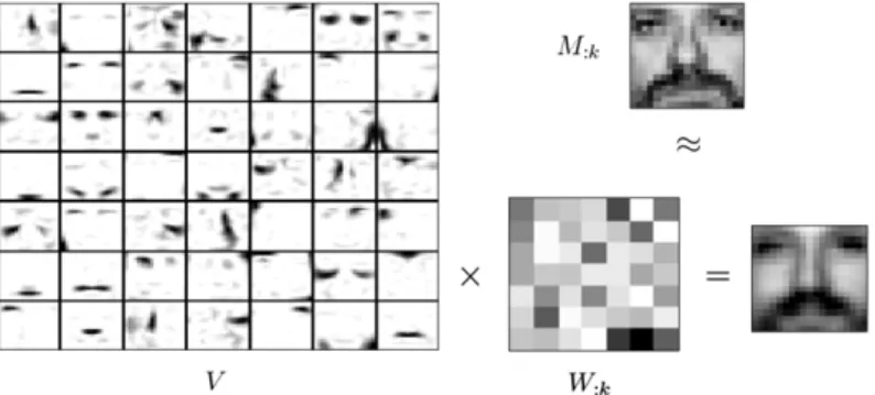
Fig. 1. Illustration of NMF on a face database. Basis elements (matrixV) obtained with NMF on the CBCL Face Database #1, MIT Center For Biological and Computation Learning, available athttp://cbcl.mit.edu/cbcl/software-datasets/FaceData2.html, consisting of 2429 gray-level images of faces (columns) with 19×19 pixels (rows), for which we set the factorization rank equal tor=49.

in the same way. Moreover, the additive reconstruction due to nonnegativity of coefficientsWkj leads to a part-based

representation[2]: basis elementsV:kwill tend to represent common parts of the columns ofM. For example, let each column

ofMbe a vectorized gray-level image of a face using (nonnegative) pixel intensities. The nonnegative matrix factorization ofMwill generate a matrixVwhose columns are nonnegative basis elements of the original images, which can then be interpreted as images as well. Moreover, since each original face is reconstructed through a weighted sum of these basis elements, the latter will provide common parts extracted from the original faces, such as eyes, noses and lips.Fig. 1illustrates this property of the NMF decomposition.

One of the main challenges of NMF is to design fast and efficient algorithms generating the nonnegative factors. In fact, on the one hand, practitioners need to compute rapidly good factorizations for large-scale problems (e.g., in text mining or image processing); on the other hand, NMF is a NP-hard problem [3] and we cannot expect to find a globally optimal solution in a reasonable computational time. This paper presents a general framework based on a multilevel strategy leading to faster initial convergence of NMF algorithms when dealing with data admitting a simple approximate low-dimensional representation (using linear transformations preserving nonnegativity), such as images. In fact, in these situations, a hierarchy of lower-dimensional problems can be constructed and used to compute efficiently approximate solutions of the original problem. Similar techniques have already been used for other dimensionality reduction tasks such as PCA [4].

The paper is organized as follows: NMF is first formulated as an optimization problem and three well-known algorithms (ANLS, MU and HALS) are briefly presented. We then introduce the concept of multigrid/multilevel methods and show how and why it can be used to speed up NMF algorithms. Finally, we experimentally demonstrate the usefulness of the proposed technique on several standard image databases, and conclude with some remarks on limitations and possible extensions of this approach.

2. Algorithms for NMF

NMF is typically formulated as a nonlinear optimization problem with an objective function measuring the quality of the low-rank approximation. In this paper, we consider the sum of squared errors:

min V∈Rm×r

W∈Rr×n

‖

M

−

VW

‖

2_F s.t. V

≥

0

,

W

≥

0

,

(NMF)

i.e., use the squared Frobenius norm

‖

A

‖

2

F

=

∑

i,jA2ijof the approximation error. Since this standard formulation of(NMF)

is NP-hard [3], most NMF algorithms focus on finding locally optimal solutions. In general, only convergence to stationary points of(NMF)(points satisfying the necessary first-order optimality conditions) is guaranteed.

2.1. Alternating nonnegative least squares (ANLS)

Although(NMF) is a nonconvex problem, it is convex separately in each of the two factorsV and W, i.e., finding the optimal factorVcorresponding to a fixed factorW reduces to a convex optimization problem, and vice-versa. More precisely, this convex problem corresponds to a nonnegative least squares (NNLS) problem, i.e., a least squares problem with nonnegativity constraints. The so-called alternating nonnegative least squares (ANLS) algorithm for(NMF)minimizes (exactly) the cost function alternatively over factorsVandWso that a stationary point of(NMF)is obtained in the limit [5]. A frequent strategy to solve the NNLS subproblems is to use active-set methods [6] (seeAppendix) for which an efficient implementation1_{is described in [9,5]. We refer the reader to [10] for a survey about NNLS methods.}

1 Available athttp://www.cc.gatech.edu/~hpark/. Notice that an improved version based on a principal block pivoting method has been released recently, see [7,8], and for which our multilevel method is also applicable, see Section7.1.

Algorithm 1Alternating nonnegative least squares

Require: Data matrixM

∈

_Rm₊×nand initial iterateW

∈

_Rr₊×n. 1: whilestopping criterion not metdo

2: V

←

argmin_V≥0

‖

M

−

VW

‖

2F; 3: W

←

argmin_W≥0

‖

M

−

VW

‖

2F. 4: end while

2.2. Multiplicative updates (MU)

In [11] Lee and Seung propose multiplicative updates (MU) for(NMF)which guarantee nonincreasingness of the objective function (cf. Algorithm 2). They also alternatively updateVforWfixed and vice versa, using a technique which was originally proposed by Daube-Witherspoon and Muehllehner to solve nonnegative least squares problems [12]. The popularity of this algorithm came along with the popularity of NMF. Algorithm 2 does not guarantee convergence to a stationary point (although it can be slightly modified in order to get this property [13,14]) and it has been observed to converge relatively slowly, see [15] and the references therein.

Algorithm 2Multiplicative Updates

Require: Data matrixM

∈

_Rm₊×nand initial iterates

(

V

,

W

)

∈

_Rm₊×r

×

_Rr₊×n. 1: whilestopping criterion not metdo

2: V

←

V

◦

[MWT]

[V(WWT_)];

3: W

←

W

◦

[VTM] [(VT_V)W].

4: end while

◦

(resp.[_[._.]_]) denotes the component-wise multiplication (resp. division).

2.3. Hierarchical Alternating Least Squares (HALS)

In ANLS, variables are partitioned at each iteration such that each subproblem is convex. However, the resolution of these convex NNLS subproblems is nontrivial and relatively expensive. If we optimize instead one single variable at a time, we get a simple univariate quadratic problem which admits a closed-form solution. Moreover, since the optimal value of each entry ofV(resp.W) does not depend of the other entries of the same column (resp. row), one can optimize alternatively whole columns ofVand whole rows ofW. This method was first proposed in [16,17] and independently by [18–20], and is herein referred to as Hierarchical Alternating Least Squares (HALS), see Algorithm 3. Under some mild assumptions, every limit point is a stationary point of(NMF), see [21].

Algorithm 3Hierarchical Alternating Least Squares

Require: DataM

∈

_Rm₊×nand initial iterates

(

V

,

W

)

∈

_Rm₊×r

×

_Rr₊×n. 1: whilestopping criterion not metdo

2: ComputeA

=

MWT_andB

₌

_WWT_. 3: fork

=

1

:

rdo 4: V:k

←

max



0

,

A:k− ∑r l=1,l̸=kV:lBlk Bkk



; 5: end for 6: ComputeC

=

VTMandD

=

VTV. 7: fork

=

1

:

rdo 8: Wk:

←

max



0

,

Ck:− ∑r l=1,l̸=kDklWl: Dkk



; 9: end for 10: end while 3. Multigrid methods

In this section, we briefly introduce multigrid methods. The aim is to give the reader some insight on these techniques in order to comprehend their applications for NMF. We refer the reader to [22–25] and the references therein for detailed discussions on the subject.

Multigrid methods were initially used to develop fast numerical solvers for boundary value problems. Given a differential equation on a continuous domain with boundary conditions, the aim is to find an approximation of asmoothfunctionf

satisfying the constraints. In general, the first step is to discretize the continuous domain, i.e., choose a set of points (a

grid) where the function values will be approximated. Then, a numerical method (e.g., finite differences, finite elements) translates the continuous problem into a (square) system of linear equations:

findx

∈

_Rn s.t. Ax

=

b

,

withA

∈

_Rn×n

,

b

∈

_Rn

,

(1)

where the vectorxwill contain the approximate values off on the grid points. Linear system(1)can be solved either by direct methods (e.g., Gaussian elimination) or iterative methods (e.g., Jacobi and Gauss–Seidel iterations). Of course, the computational cost of these methods depends on the number of points in the grid, which leads to a trade-off between precision (number of points used for the discretization) and computational cost.

Iterative methods update the solution at each step and hopefully converge to a solution of(1). Here comes the utility of multigrid: instead of working on a fine grid during all iterations, the solution isrestrictedto a coarser grid2_{on which the}

iterations are cheaper. Moreover, the smoothness of functionf allows to recover its low-frequency components faster on coarser grids. Solutions of the coarse grid are thenprolongatedto the finer grid and iterations can continue (higher frequency components of the error are reduced faster). Because the initial guess generated on the coarser grid is a good approximation of the final solution, less iterations are needed to converge on the fine (expensive) grid. Essentially, multigrid methods make iterative methods more efficient, i.e., accurate solutions are obtained faster.

More recently, these same ideas have been applied to a broader class of problems, e.g., multiscale optimization with trust-region methods [26] and multiresolution techniques in image processing [27].

4. Multilevel approach for NMF

The three algorithms presented in Section2(ANLS, MU and HALS) are iteratively trying to find a stationary point of (NMF). Indeed, most practical NMF algorithms areiterative methods, such as projected gradient methods [28] and Newton-like methods [29,30] (see also [31–33,18] and the references therein). In order to embed these algorithms in a multilevel strategy, one has to define the different levels and describe how variables and data are transferred between them. In this section, we first present a general description of the multilevel approach for NMF algorithms, and then apply it to image datasets.

4.1. Description

Let each column of the matrixMbe a element of the dataset (e.g., a vectorized image) belonging toRm+. We define the restriction operatorRas a linear operator

R

:

_Rm₊

→

_Rm₊′

:

x

→

R

(

x

)

=

Rx

,

withR

∈

_R+m′×mandm′

_<

_{m, and the prolongationPas a linear operator} P

:

_Rm₊′

→

_Rm₊

:

y

→

P

(

y

)

=

Py

,

withP

∈

_Rm₊×m′. Nonnegativity of matricesRandPis a sufficient condition to preserve nonnegativity of the solutions when they are transferred from one level to another. In fact, in order to generate nonnegative solutions, one requires

R

(

x

)

≥

0

,

∀

x

≥

0 and P

(

y

)

≥

0

,

∀

y

≥

0

.

We also define the corresponding transfer operators on matrices, operating columnwise: R(

[

x1x2

· · ·

xn

]

)

= [

R(x1

)R(

x2

)

· · ·

R(xn

)

]

,

and

P

(

[

y1y2

· · ·

yn

]

)

= [

P

(

y1

)

P

(

y2

)

· · ·

P

(

yn

)

]

,

forxi

∈

Rm+

,

yi

∈

Rm ′

+

,

1

≤

i

≤

n.

In order for the multilevel strategy to work, information lost when transferring from one level to another must be limited, i.e., data matrixMhas to be well represented byR(M

)

in the lower dimensional space, which means that the reconstruction P

(

R

(

M

))

must be close toM. From now on, we say thatMis smooth with respect toRandPif and only if

sM

=

‖

M

−

P

(R(

M

))

‖

_F

‖

M

‖

_F is small

.

QuantitysMmeasures how wellMcan be mapped byRinto a lower-dimensional space, then brought back byP, and

still be a fairly good approximation of itself.

Based on these definitions, elaborating a multilevel approach for NMF is straightforward: 1. We are givenM

∈

_Rm₊×nand

(

V0

,

W0

)

∈

Rm+×r

×

Rr

×n + . 2. ComputeM′

₌

_R

₍

_M

₎

₌

_RM

_∈

Rm ′_×n + andV0′

=

R

(

V0

)

=

RV0

∈

Rm ′_×r

+ , i.e., restrict the elements of the dataset and the basis elements of the current solution to a lower dimensional space.

3. Compute a rank-rNMF

(

V′

_,

_W

₎

_ofM′_using

₍

_V′

0

,

W0

)

as initial matrices, i.e.,

V′W

≈

M′

=

R

(

M

).

This can be done using any NMF iterative algorithm or, even better, using the multilevel strategy recursively (cf. Section4.3).

4. Since

M

≈

P

(

R

(

M

))

=

P

(

M′

)

≈

P

(

V′W

)

=

PV′W

=

P

(

V′

)

W

=

VW

,

whereV is the prolongation ofV′

_{, (}

_V

_,

_W

₎

_{is a good initial estimate for a rank-rNMF ofM,provided that Mis smooth} with respect toRandP(i.e.,sMis small) and thatV′W is a good approximation ofM′

=

R

(

M

)

(i.e.,

‖

M′

−

V′W

‖

Fis

small); in fact,

‖

M

−

P

(

V′

)

W

‖

_F

≤ ‖

M

−

P

(

R

(

M

))

‖

_F

+ ‖

P

(

R

(

M

))

−

P

(

V′W

)

‖

_F

≤

sM

‖

M

‖

F

+ ‖

P

(

R

(

M

)

−

V′W

)

‖

F

≤

sM

‖

M

‖

F

+ ‖

P

‖

F

‖

M′

−

V′W

‖

F

.

5. Further improve the solution

(

V

,

W

)

using any NMF iterative algorithm.

Computations needed at step 3 are cheap (sincem′

<

m) and, moreover, the low-frequency components of the error3 are reduced faster on coarse levels (cf. Section4.4). Therefore this strategy is expected to accelerate the convergence of NMF algorithms.

We now illustrate this technique on image datasets, more precisely, on two-dimensional gray-level images. In general, images are composed of several smooth components, i.e., regions where pixel values are similar and change continuously with respect to their location (e.g., skin on a face or the pupil, or sclera,4 of an eye). In other words, a pixel value can often be approximated using the pixel values of its neighbors. This observation can be used to define the transfer operators (Section4.2). For the computation of a NMF solution, the multilevel approach can be used recursively; three strategies (called multigrid cycles) are described in Section4.3. Finally, numerical results are reported in Section5.

4.2. Coarse grid and transfer operators

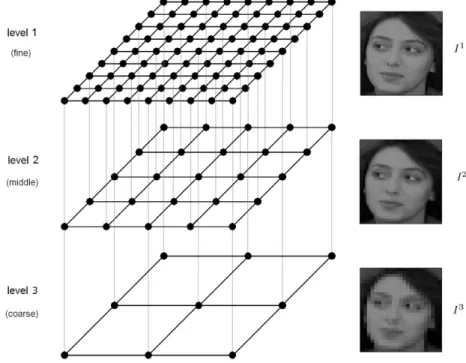
A crucial step of multilevel methods is to define the different levels and the transformations (operators) between them. Fig. 2is an illustration of a standardcoarse griddefinition: we noteI1the matrix of dimension

(

2a

+1

)

×

(

2b

+1

)

representing the initial image andIl_{the matrix of dimension}

₍

₂a−l+1

₊

₁

₎

_×

₍

₂b−l+1

₊

₁

₎

_{representing the image at levellobtained by}

keeping, in each direction, only one out of every two points of the grid at the preceding level, i.e.,Il−1_.

The transfer operators describe how to transform the images when going from finer to coarser levels, and vice versa, i.e., how to compute the values (pixel intensities) of the imageIl_{using values from imageI}l−1_{at the finer level (restriction)}

or from imageIl+1at the coarser level (prolongation). For therestriction, thefull-weightingoperator is a standard choice: values of the coarse grid points are the weighted averages of the values of their neighbors on the fine grid (seeFig. 3for an illustration). NotingIl

i,jthe intensity of the pixel

(

i

,

j

)

of imageIl, it is defined as follows:

I_il_,+_j1

=

1 16



I₂l_i−1,2j−1

+

I l 2i−1,2j+1

+

I l 2i+1,2j−1

+

I l 2i+1,2j+1

+

2

(

I l 2i,2j−1

+

I l 2i−1,2j

+

I l 2i+1,2j

+

I l 2i,2j+1

)

+

4I l 2i,2j



,

(2) except on the boundaries of the image (wheni

=

0

,

j

=

0

,

i

=

2a−l+1and/orj

=

2b−l+1) where the weights are adapted correspondingly. For example, to restrict a 3

×

3 image to a 2

×

2 image,Ris defined with

R

=

1 9







4 2 0 2 1 0 0 0 0 0 2 4 0 1 2 0 0 0 0 0 0 2 1 0 4 2 0 0 0 0 0 1 2 0 2 4







(3

×

3 images needing first to be vectorized to vectors inR9, by concatenation of either columns or rows).

3 The low-frequency components refer to the parts of the data which are well-represented on coarse levels. 4 The white part of the eye.

Fig. 2. Multigrid Hierarchy. Schematic view of a grid definition for image processing (image from ORL face database, cf. Section5).

Fig. 3. Restriction and prolongation.

For theprolongation, we set the values on the fine grid points as the average of the values of their neighbors on the coarse grid: I_il_,j

=

meani′ ∈rd(i/2) j′ ∈rd(j/2)



I_il′+_,j1′



,

(3) where rd

(

k

/

2

)

=



{

k

/

2} keven,

{

(

k

−

1

)/

2

, (

k

+

1

)/

2} kodd

.

For example, to prolongate a 2

×

2 image to a 3

×

3 image,Pis defined with

PT

=

1 4







4 2 0 2 1 0 0 0 0 0 2 4 0 1 2 0 0 0 0 0 0 2 1 0 4 2 0 0 0 0 0 1 2 0 2 4







.

Note that these transformations clearly preserve nonnegativity.

4.3. Multigrid cycle

Now that grids and transfer operators are defined, we need to choose the procedure that is applied at each grid level as it moves through the grid hierarchy. In this section, we propose three different approaches: nested iteration, V-cycle and full multigrid cycle.

In our setting, the transfer operators only change the number of rowsmof the input matrixM, i.e., the number of pixels in the images of the database: the size of the images are approximatively four times smaller between each level:m′

≈

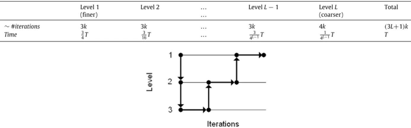
1

Table 1

Number of iterations performed and time spent at each level when allocating amongLlevels a total computational budgetT, corresponding to 4kiterations at the finest level.

Level 1 Level 2 . . . LevelL−1 LevelL Total

(finer) . . . (coarser) ∼#iterations 3k 3k . . . 3k 4k (3L+1)k Time 3 4T 3 16T . . . 3 4L−1T 1 4L−1T T

Fig. 4. Nested iteration. Transition between different levels for nested iteration.

When the number of images in the input matrix is not too large, i.e., whenn

≪

m, the computational complexity per iteration of the three algorithms (ANLS, MU and HALS) is close to being proportional tom(cf.Appendix), and the iterations will then be approximately four times cheaper (see also Section6.1). A possible way to allocate the time spent at each level is to allow the same number of iterations at each level, which seems to give good results in practice.Table 1shows the time spent and the corresponding number of iterations performed at each level.

Note that the transfer operators requireO

(

mn

)

operations and, since they are only performed once between each level, their computational cost can be neglected (at least forr

≫

1 and/or when a sizable amount of iterations are performed).

4.3.1. Nested iteration (NI)

To initialize NMF algorithms, we propose to factorize the image at the coarsest resolution and then use the solution as initial guess for the next (finer) resolution. This is referred to asnested iteration, seeFig. 4for an illustration with three levels and Algorithm 4 for the implementation. The idea is to start off the final iterations at the finer level with a better initial estimate, thus reducing the computational time required for the convergence of the iterative methods on the fine grid. The number of iterations and time spent at each level is chosen according toTable 1, i.e., three quarters of the alloted time for iterations at the current level preceded by one quarter of the time for the recursive call to the immediately coarser level. Algorithm 4Nested Iteration

Require: L

∈

_N(number of levels),M

∈

_Rm₊×n(data matrix),

(

V0

,

W0

)

∈

Rm+×r

×

Rr ×n

+ (initial matrices) andT

≥

0 (total time allocated to the algorithm).

Ensure:

(

V

,

W

)

≥

0 s.t.VW

≈

M. 1: ifL

=

1then 2:

[

V

,

W

] =

NMF algorithm

(

M

,

V0

,

W0

,

T

)

; 3: else 4: M′

₌

_R

₍

_M

₎

_;V′ 0

=

R

(

V0

)

; 5:

[

V′

,

W

] =

Nested Iteration

(

L

−

1

,

M′

,

V₀′

,

W0

,

T

/

4

)

; 6: V

=

P

(

V′

₎

_; 7:

[

V

,

W

] =

NMF algorithm

(

M

,

V

,

W

,

3T

/

4

)

; 8: end if

Remark 1. When the ANLS algorithm is used, the prolongation ofV′_{does not need to be computed since that algorithm} only needs an initial value for theWiterate. Note that this can be used in principle to avoid computing any prolongation, by settingVdirectly as the optimal solution of the corresponding NNLS problem.

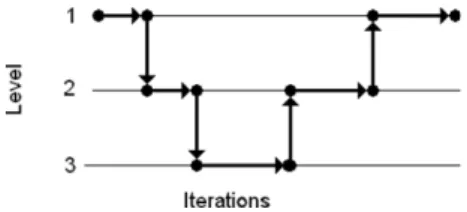
4.3.2. V-cycle (VC)

One can often empirically observe that multilevel methods perform better if a few iterations are performed at the fine level immediately before going to coarser levels. This is partially explained by the fact that these first few iterations typically lead to a relatively important decrease of the objective function, at least compared to subsequent iterations. A simple application of this strategy is referred to as V-cycle and is illustrated onFig. 5with three levels; see Algorithm 5 for the implementation. Time allocation is as follows: one quarter of the alloted time is devoted to iterations at the current level,

Fig. 5. V-cycle. Transition between different levels for V-cycle.

followed by one quarter of the time for the recursive call to the immediately coarser level, and finally one half of the time again for iterations at the current level (we have therefore three quarters of the total time spent for iterations at current level, as for nested iteration).

Algorithm 5V-cycle

Require: L

∈

_N(number of levels),M

∈

_Rm₊×n(data matrix),

(

V0

,

W0

)

∈

Rm+×r

×

Rr ×n

+ (initial matrices) andT

≥

0 (total time allocated to the algorithm).

Ensure:

(

V

,

W

)

≥

0 s.t.VW

≈

M. 1: ifL

=

1then 2:

[

V

,

W

] =

NMF algorithm

(

M

,

V0

,

W0

,

T

)

; 3: else 4:

[

V

,

W

] =

NMF algorithm

(

M

,

V0

,

W0

,

T

/

4

)

; 5: M′

=

R

(

M

)

;V′

=

R

(

V

)

; 6:

[

V′

_,

_W

_{] =}

_V-cycle

₍

_L

₋

₁

_,

_M′

_,

_V′

_,

_W

_,

_T

_/

₄

₎

_; 7: V

=

P

(

V′

₎

_; 8:

[

V

,

W

] =

NMF algorithm

(

M

,

V

,

W

,

T

/

2

)

; 9: end if 4.3.3. Full multigrid (FMG)

Combining ideas of nested iteration and V-cycle leads to a full multigrid cycle defined recursively as follows: at each level, a V-cycle is initialized with the solution obtained at the underlying level using a full-multigrid cycle. This is typically the most efficient multigrid strategy [25]. In this case, we propose to partition the time as follows (Tis the total time):T₄for the initialization (call of the full multigrid on the underlying level) and3₄T for the V-cycle at the current level (cf. Algorithm 6). Algorithm 6Full Multigrid

Require: L

∈

_N(number of levels),M

∈

_R+m×n(data matrix),

(

V0

,

W0

)

∈

Rm+×r

×

Rr+×n(initial matrices) andT

≥

0 (total time allocated to the algorithm).

Ensure:

(

V

,

W

)

≥

0 s.t.VW

≈

M. 1: ifL

=

1then 2:

[

V

,

W

] =

NMF algorithm

(

M

,

V0

,

W0

,

T

)

; 3: else 4: V′

₌

_R

₍

_V 0

)

;M′

=

R

(

M

)

; * 5:

[

V′

_,

_W

_{] =}

_{Full Multigrid}

₍

_L

₋

₁

_,

_M′

_,

_V′

_,

_W 0

,

T

/

4

)

; 6: V

=

prolongation

(

V′

)

; 7:

[

V

,

W

] =

V-cycle

(

L

,

M

,

V

,

W

,

3T

/

4

)

; 8: end if

*Note that the restrictions ofMshould be computed only once for each level and saved as global variables so that the call of the V-cycle (step 7) does not have to recompute them.

4.4. Smoothing properties

We explained why the multilevel strategy was potentially able to accelerate iterative algorithms for NMF: cheaper computations and smoothing of the error on coarse levels. Before giving extensive numerical results in Section5, we illustrate these features of multilevel methods on the ORL face database.

Comparing three levels,Fig. 6 displays the error (after prolongation to the fine level) for two faces and for different numbers of iterations (10, 50 and 100) using MU. Comparing the first row and the last row ofFig. 6, it is clear that, in this example, the multilevel approach allows a significant smoothing of the error. After only 10 iterations, the error obtained

Fig. 6. Smoothing on coarse levels. Example of the smoothing properties of the multilevel approach on the ORL face database. Each image represents the absolute value of the approximation error (black tones indicate a high error) of one of two faces from the ORL face database. These approximations are the prolongations (to the fine level) of the solutions obtained using the multiplicative updates on a single level, with factorization rankr=40 and the same initial matrices. From top to bottom: level 1 (fine), level 2 (middle) and level 3 (coarse); from left to right: 10 iterations, 50 iterations and 100 iterations.

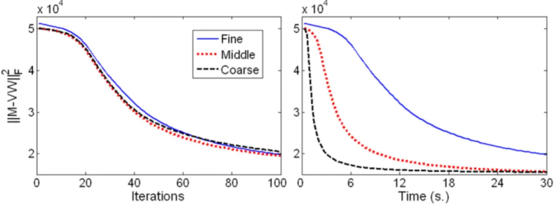
Fig. 7. Evolution of the error on each level, after prolongation on the fine level, with respect to (left) the number of iterations performed and (right) the computational time. Same setting as inFig. 6.

Table 2 Image datasets. Data # pixels m n r ORL facea _{112×92 10 304 400 40} Umist faceb _{112×92 10 304 575 40} Irisc _{960×1280 1 228 800 8 4} Hubble telescope [34] 128×128 16 384 100 8 a_{http://www.cl.cam.ac.uk/research/dtg/attarchive/facedatabase.html.} b_{http://www.cs.toronto.edu/~roweis/data.html.} c_{http://www.bath.ac.uk/elec-eng/research/sipg.}

with the prolongated solution of the coarse level is already smoother and smaller (seeFig. 7), while it is computed much faster.

Fig. 7 gives the evolution of the error with respect to the number of iterations performed (left) and with respect to computational time (right). In this example, the initial convergence on the three levels is comparable, while the computational cost is much cheaper on coarse levels. In fact, compared to the fine level, the middle (resp. coarse) level is approximately 4 (resp. 16) times cheaper.

5. Computational results

To evaluate the performance of our multilevel approach, we present some numerical results for several standard image databases described inTable 2.

Table 3

Comparison of the mean error on the 100 runs with ANLS.

# lvl ORL Umist Iris Hubble

NMF 1 14 960 26 013 28 934 24.35 NI 2 14 683 25 060 27 834 15.94 3 14 591 24 887 27 572 16.93 4 14 580 24 923 27 453 17.20 VC 2 14 696 25 195 27 957 16.00 3 14 610 24 848 27 620 16.12 4 14 599 24 962 27 490 16.10 FMG 2 14 683 25 060 27 821 16.10 3 14 516 24 672 27 500 16.56 4 14 460 24 393 27 359 16.70 Table 4

Comparison of the mean error on the 100 runs with MU.

# lvl ORL Umist Iris Hubble

NMF 1 34 733 131 087 64 046 21.68 NI 2 23 422 87 966 37 604 22.80 3 20 502 67 131 33 114 18.49 4 19 507 59 879 31 146 16.19 VC 2 23 490 90 064 36 545 10.62 3 20 678 69 208 32 086 9.77 4 19 804 62 420 30 415 9.36 FMG 2 23 422 87 966 37 504 22.91 3 19 170 58 469 32 120 15.06 4 17 635 46 570 29 659 11.71 Table 5

Comparison of the mean error on the 100 runs with HALS.

# lvl ORL Umist Iris Hubble

NMF 1 15 096 27 544 31 571 17.97 NI 2 14 517 25 153 29 032 17.37 3 14 310 24 427 28 131 16.91 4 14 280 24 256 27 744 16.92 VC 2 14 523 25 123 28 732 17.37 3 14 339 24 459 28 001 17.02 4 14 327 24 364 27 670 17.04 FMG 2 14 518 25 153 29 120 17.39 3 14 204 23 950 27 933 16.69 4 14 107 23 533 27 538 16.89

For each database, the three multigrid cycles (NI, V-cycle and FMG) of our multilevel strategy are tested using 100 runs initialized with the same random matrices for the three algorithms (ANLS, MU and HALS), with a time limit of 10 s. All algorithms have been implemented in MATLAB⃝r _{7.1 (R14) and tested on a 3 GHz Intel}⃝r _CoreTM_{2 Dual CPU PC.}

5.1. Results

Tables 3–5give the mean error attained within 10 s using the different approaches. In all cases, the multilevel approach generates much better solutions than the original NMF algorithms, indicating that it is able to accelerate their convergence. The full multigrid cycle is, as expected, the best strategy while nested iteration and V-cycle give comparable performances. We also observe that the additional speedup of the convergence when the number of levels is increased from 3 to 4 is less significant; it has even a slightly negative effect in some cases. In general, the ‘optimal’ number of levels will depend on the smoothness and the size of the data, and on the algorithm used (cf. Section6.1).

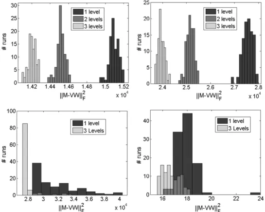
HALS combined with the full multigrid cycle is one of the best strategies.Fig. 8displays the distribution of the errors for the different databases in this particular case. For the ORL and Umist databases, the multilevel strategy is extremely efficient: all the solutions generated with 2 and 3 levels are better than the original NMF algorithm. For the Iris and Hubble databases, the difference is not as clear. The reason is that the corresponding NMF problems are ‘easier’ because the factorization rankris smaller. Hence the algorithms converge faster to stationary points, and the distribution of the final errors is more concentrated.

Fig. 8. Distribution of the error among the 100 random initializations using the HALS algorithm with a full multigrid cycle: (top left) ORL, (top right) Umist, (bottom left) Iris, and (bottom right) Hubble.

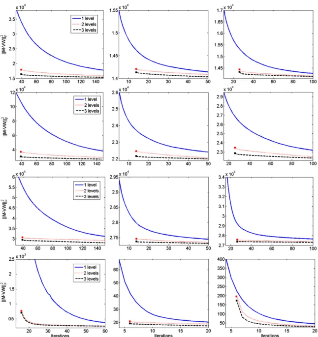
In order to visualize the evolution of the error through the iterations,Fig. 9plots the objective function with respect to the number of iterations independently for each algorithm and each database, using nested iteration as the multigrid cycle (which is the easiest to represent). In all cases, prolongations of solutions from the lower levels generate much better solutions than those obtained on the fine level (as explained in Section4.4).

These test results are very encouraging: the multilevel approach for NMF seems very efficient when dealing with image datasets and allows a significant speedup of the convergence of the algorithms.

6. Limitations

Although the numerical results reported in the previous section demonstrate significant computational advantages for our multilevel technique, we point out in this section two limitations that can potentially affect our approach.

6.1. Size of the data matrix

The approach described above was applied to only one dimension of the input data: restriction and prolongation operators are applied to columns of the input matrixMand of the first factorV. Indeed, we assumed that each of these columns satisfies some kind of smoothness property. In contrast, we did not assume that the columns ofMare related to each other in any way, so that no such property holds for the rows ofM. Therefore we did not apply our multilevel strategy along the second dimension of the input data, and our approach only reduced the row dimension of matrixMat each level frommtom′

_≈

m

4, while the column dimensionnremained the same.

The fact that the row dimension of factorVbecomes smaller at deeper levels clearly implies that the computational cost associated with updatingVwill decrease. This reduction is however not directly proportional to the reduction fromm

tom′, as this cost also depends on the factorization rankrand the dimensions of the other factor, which are not affected. Similarly, although the dimensions of factorWremain the same regardless of the depth, its updates could become cheaper because dimensionmalso plays a role there. The relative extent of those effects depends on the NMF algorithm used, and will determine in which situations a reduction in the dimensionmis clearly beneficial with respect to the whole computational cost of the algorithm.

We now analyze in detail the effect of a reduction ofmon the computational cost of one iteration of the algorithms presented in Section2:

Fig. 9. Evolution of the objective function. From left to right: MU, ANLS and HALS. From top to bottom: ORL, Umist, Iris and Hubble databases. 1levelstands for the standard NMF algorithms. The initial points for the curves 2levelsand 3levelsare the prolongated solutions obtained on the coarser levels using nested iteration, cf. Section4.3. All algorithms were initialized with the same random matrices.

Table 6

Number of floating point operations needed to updateVandWin ANLS, MU and HALS.

ANLS MU and HALS

Update ofV O(mnr+ms(r)r3_+nr2_{) O(mnr+(m+n)r}2₎

Update ofW O(mnr+ns(r)r3_+mr2_{) O(mnr+(m+n)r}2₎

Both updates O(m(nr+s(r)r3_)+ns(r)r3_{) O(m(nr+r}2_)+nr2₎

(Functions(r)is 2r_{in the worst case, and typically much smaller, seeAppendix.)}

Table 6gives the computational cost for the updates ofVandWseparately, as well as their combined cost (seeAppendix). Our objective is to determine for which dimensions

(

m

,

n

)

of the input matrix and for which rankrour multilevel strategy (applied only to the row dimensionm) is clearly beneficial or, more precisely, find when a constant factor reduction inm, say_mm′

=

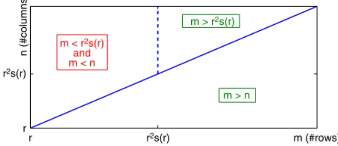
4, leads to a constant factor reduction in the total computational cost of both updates. We make the following

r2_s(r) r2_s(r) r r m (#rows) n (#columns) m < r 2_s(r) and m < n m > n m > r2_s(r)

Fig. 10. Regions for input dimensions(m,n)where a multilevel strategy is beneficial in all cases (m≥min{n,r2_{s(r)}, lower and upper right parts) or only}

for MU and HALS (m≤min{n,r2_{s(r)}, upper left part).} observations, illustrated onFig. 10.

•

We need only consider the region where bothmandnare greater than the factorization rankr(otherwise the trivial factorization with an identity matrix is optimal).

•

Looking at the last row of the table, we see that all terms appearing in the combined computational cost for both updates are proportional tom, except for two terms:ns

(

r

)

r3_{for ANLS andnr}2_{for MU and HALS. If the contributions of those}

two terms could be neglected compared to the total cost, any constant factor reduction in dimensionmwould lead to an equivalent reduction in the total complexity, which is the ideal situation for our multilevel strategy.

•

Whenm

≥

n, termsns

(

r

)

r3 _{for ANLS andnr}2 _{for MU and HALS are dominated respectively byms}

₍

_r

₎

_r3 _{and mr}2

(i.e.,ns

(

r

)

r3

_≤

_ms

₍

_r

₎

_r3_andnr2

_≤

_mr2_{), so that they cannot contribute more than half of the total computational}

cost. Therefore a reduction in dimensionmwill guarantee a constant factor reduction in the total complexity. Let us illustrate this on the MU (a similar analysis holds for ANLS and HALS) for which the exact total computational cost is 2m

(

nr

+

r2

₎

₊

_2nr2_{(seeAppendix). The factor reductionf}

MUin the total complexity satisfies

1

≤

fMU

=

m

(

nr

+

r2

)

+

nr2 m′

₍

_nr

₊

_r2

₎

₊

_nr2

≤

m

m′

=

4

,

and, form

≥

n

≥

rand_mm′

=

4, we have that

fMU

≥

mnr

+

mr2

₊

_mr2 m′_nr

₊

_m′_r2

₊

_mr2

=

4m′_nr

₊

_8m′_r2 m′_nr

₊

_5m′_r2

≥

4m′_r2

₊

_8m′_r2 m′_r2

₊

_5m′_r2

=

2

,

i.e., the total computational cost of the MU updates on the coarse level is at least twice cheaper than on the fine level. Moreover, whenmis much larger thann

(

m

≫

n

)

, as is the case for our images, the terms inncan be neglected, and we find ourselves in the ideal situation described previously (withfMU

≈

4). In conclusion, whenm

≥

n, we always have an

appreciable reduction in the computational cost.

•

Looking now at MU and HALS whenmis smaller thann, we see that the termnr2is always dominated bymnr(i.e.,

nr2

_≤

_{mnr), becausem}

_≥

_{ralways holds. We conclude that a constant factor reduction in the total complexity can also}

be expected whenmis reduced. For example, for MU, we have

fMU

≥

mnr

+

mr2

+

mnr m′_nr

₊

_m′_r2

₊

_mnr

=

8m′nr

+

4m′r2 5m′_nr

₊

_m′_r2

≥

8 5

.

•

Considering now ANLS whenmis smaller thann, we see that the termns

(

r

)

r3_{is dominated bymnras soon asm}

_≥

_s

₍

_r

₎

_r2_.

Again, in that situation, a constant factor reduction in the total complexity can be obtained5. Finally, the only situation where the improvement due to the multilevel technique is modest when using ANLS when bothm

<

nandm

<

s

(

r

)

r2

hold, in which case the termns

(

r

)

r3_{can dominate all the others, and a reduction in dimensionmis not guaranteed to}

lead to an appreciable reduction in the total complexity.

To summarize, applying multilevel techniques to the methods presented in this paper is particularly beneficial on datasets for whichmis sufficiently large compared tonandr(for MU and HALS) and tonands

(

r

)

r2(for ANLS). Some gains can always be expected for MU and HALS, while ANLS will only see a significant improvement ifm

≥

min{n

,

s

(

r

)

r2

_}

_holds.

In Section5, we have presented computational experiments for image datasets satisfying this requirement: the number of imagesnwas much smaller than the number of pixelsmin each image. In particular, we observed that the acceleration

5 It is worth noting that whenm≥s(r)r2_{the initial computation required to formulate the NNLS subproblem inW:}

min W≥0 n − i=1 ‖M:i−VW:i‖2F = n − i=1 ‖M:i‖2F−2(M T :iV)W:i+W:Ti(V T_V)W :i, (4)

provided by the multilevel approach to the ANLS algorithm was not as significant as for HALS: while in most cases ANLS converged faster than HALS when using the original NMF algorithms, it converged slower as soon as the multilevel strategy was used (seeTables 3and5).

To end this section, we note that, in some applications, rows of matrixMcan also be restricted to lower-dimensional spaces. In these cases, the multilevel method could be made even more effective. This is the case for example in the following situations:

•

In hyperspectral images, each column of matrixMrepresents an image at a given wavelength, while each row represents the spectral signature of a pixel, see, e.g., [35,36]. Since spectral signatures feature smooth components, the multilevel strategy can be easily generalized to reduce the number of rowsnof the data matrixM.

•

For a video sequence, each column of matrixMrepresents an image at a given time so that consecutive images share similarities. Moreover, if the camera is fixed, the background of the scene is the same among all images. The multilevel approach can then also be generalized to reduce the number of columns ofMin a meaningful way.

•

In face datasets (e.g., used for face recognition), a person typically appears several times. Hence one can imagine using the multilevel strategy by merging different columns corresponding to the same person.

6.2. Convergence

In classical multigrid methods, when solving a linear system of equationsAx

=

b, the current approximate solution

xcis not transferred from a fine level to a coarser one, because it would imply the loss of its high-frequency components;

instead, the residual is transferred, which we briefly explain here. Defining the current residualrc

=

b

−

Axcand the error e

=

x

−

xc, we have the equivalent defect equationAe

=

rcand we would like to approximateewith a correctionecin

order to improve the current solution withxc

←

xc

+

ec. The defect equation is solved approximately on the coarser grid

by restricting the residualrc, the correction obtained on the coarser grid is prolongated and the new approximationxc

+

ec

is computed, see, e.g., [25, p. 37]. If instead the solution is transferred directly from one level to another (as we do in this paper), the corresponding scheme is in general not convergent, see [25, p. 156]. In fact, even an exact solution of the system

Ax

=

bis not a fixed point, because the restriction ofxis not an exact solution anymore at the coarser level (while, in that case, the residualris equal to zero and the correctionewill also be equal to zero).

Therefore, the method presented in this paper should in principle only be used as apre-processingorinitializationstep before another (convergent) NMF algorithm is applied. In fact, if one already has a good approximate solution

(

V

,

W

)

for NMF (e.g., a solution close to a stationary point), transferring it to a coarser grid will most likely increase the approximation error because high frequency components (such as edges in images) will be lost. Moreover, it seems that the strategy of transferring a residual instead of the whole solution is not directly applicable to NMF. Indeed, a ‘local linearization’ approach, which would consist in linearizing the equation

M

−

(

V

+

1V

)(

W

+

1W

)

≈

0

⇐⇒

R

=

M

−

VW

≈

V1W

+

1VW

,

where1Vand1Ware the corrections to be computed on the coarser grids, causes several problems. First, handling non-negativity of the coarse versions of the factors becomes non-trivial. Second, performing this approximation efficiently also becomes an issue, since for example computing the residualRis as expensive as computing directly a full MU or HALS iteration on the fine grid (O

(

mnr

)

operations). Attempting to fix these drawbacks, which seems to be far from trivial, is a topic for further research.

To conclude this section, we reiterate that, despite these theoretical reservations, it seems our technique is still quite efficient (see Section5). One reason that explains that good behavior is that NMF solutions are typicallypart-basedand

sparse[2], seeFig. 1. Therefore, columns of matrixV contains relatively large ‘constant components’, made of their zero

entries, which are perfectly transferred from one level to another, so thatsV

=

‖V−P(R(V))‖F

‖V‖F will typically be very small (in general much smaller thansM).

7. Concluding remarks

In this paper, a multilevel approach designed to accelerate NMF algorithms has been proposed and its efficiency has been experimentally demonstrated. Applicability of this technique relies on the ability to design linear operators preserving nonnegativity and transferring accurately data between different levels. To conclude, we give some directions for further research.

7.1. Extensions

We have only used our multilevel approach for a specific objective function (sum of squared errors) to speed up three NMF algorithms (ANLS, MU and HALS) and to factorize 2D images. However, this technique can be easily generalized to different objective functions, other iterative algorithms and applied to various kinds of smooth data. In fact, the key characteristic we exploit is the fact that a reduction of the dimension(s) of the input matrix (in our numerical examples,m) leads to cheaper

iterations (on coarse levels) for any reasonable algorithm, i.e., any algorithm whose computational cost depends on the dimensions of the input matrix (see also the more detailed analysis in Section6.1).

Moreover, other types of coarse grid definition (e.g., red–black distribution), transfer operators (e.g., wavelets transform) and grid cycle (e.g., W-cycle or flexible cycle) can be used and could potentially further improve efficiency.

This idea can also be extended to nonnegative tensor factorization (NTF), see, e.g., [32,34] and the references therein, by using multilevel techniques for higher-dimensional spaces.

7.2. Initialization

Several judicious initializations for NMF algorithms have been proposed in the literature which allow to accelerate convergence and, in general, improve the final solution [37,38]. The computational cost of these good initial guesses depends on the matrix dimensions and will then be cheaper on a coarser grid. Therefore, it would be interesting to combine classical NMF initializations techniques with our multilevel approach for further speedups.

7.3. Unstructured data

When we do not possess any kind information about the matrix to factorize (and a fortiori about the solution), applying a multilevel method seems out of reach. In fact, in these circumstances, there is no sensible way to define the transfer operators.

Nevertheless, we believe it is not hopeless to extend the multilevel idea to other types of data. For example, in text mining applications, the term-by-document matrix can be restricted by stacking synonyms or similar texts together, see [4] where graph coarsening is used. This implies some a priori knowledge or preprocessing of the data and, assuming it is cheap enough, the application of a multilevel strategy could be expected to be profitable in that setting.

Acknowledgments

We thank Quentin Rentmeesters, Stephen Vavasis and an anonymous reviewer for their insightful comments which helped us to improve the paper.

This work was carried out when the first author was a Research fellow of the Fonds de la Recherche Scientifique (F.R.S.-FNRS) at Université catholique de Louvain.

Appendix. Computational cost of ANLS, MU and HALS

A.1. MU and HALS

The main computational cost for updatingVin both MU and HALS resides in the computation ofMWTand6V

(

WWT

)

, which requires respectively 2mnrand 2

(

m

+

n

)

r2_{operations, cf. Algorithms 2 and 3. UpdatingWrequires the same number}

of operations, so that the total computational cost isO

(

mnr

+

(

m

+

n

)

r2

₎

_{operations per iteration, almost proportional to}

m(only thenr2term is not, but is negligible compared to the other terms, cf. Section6.1), see also [21, Section 4.2.1].

A.2. Active-set methods for NNLS

In a nutshell, active-set methods for nonnegative least squares work in the following iterative fashion [6, Algorithm NNLS, p. 161]

0. Choose the set of active (zero) and passive (nonzero) variables.

1. Get rid of the nonnegativity constraints and solve the unconstrained least squares problem (LS) corresponding to the set of passive (nonzero) variables (the solution is obtained by solving a linear system, i.e., the normal equations).

2. Check the optimality conditions, i.e., the nonnegativity of passive variables, and the nonnegativity of the gradients of the active variables. If they are satisfied, stop.

3. Exchange variables between the set of active and the set of passive variables in such a way that the objective function is decreased at each step; and go to 1.

In(NMF), the problem of computing the optimalV for a given fixedW can be decoupled intomindependent NNLS subproblems inrvariables:

min

Vi:∈Rr+

‖

Mi:

−

Vi:W

‖

2_F

,

1

≤

i

≤

m

.

Each of them amounts to solving a sequence of linear subsystems (with at mostrvariables, cf. step 1 above) of

Vi:

(

WWT

)

=

Mi:WT

,

1

≤

i

≤

m

.

In the worst case, one might have to solve every possible subsystem, which requiresO

(

g

(

r

))

operations with7_g

₍

_r

₎

₌

∑

r

i=1



r i



i3

₌

_Θ

₍

₂r_r3

₎

_{. Note thatWW}T_andMWT_{can be computed once for all, which requiresO}

₍

_mnr

₊

_nr2

₎

_{operations (see}

previous section on MU and HALS). UpdatingVthen requiresO

(

mnr

+

ms

(

r

)

r3

₊

_nr2

₎

_{operations, while updatingWsimilarly}

requiresO

(

mnr

+

ns

(

r

)

r3

₊

_mr2

₎

_{. Finally, the total computational cost of one ANLS step isO}

₍

_mnr

₊

₍

_m

₊

_n

₎

_r2

₍

_rs

₍

_r

₎

₊

₁

₎₎

₌

O

(

mnr

+

(

m

+

n

)

s

(

r

)

r3

)

operations per iteration, wheres

(

r

)

≤

2r. The number of stepss

(

r

)

isΘ

(

2r

)

in the worst case, but in practice is typically much smaller (as is the case for the simplex method for linear programming).

References

[1] P. Paatero, U. Tapper, Positive matrix factorization: a non-negative factor model with optimal utilization of error estimates of data values, Environmetrics 5 (1994) 111–126.

[2] D. Lee, H. Seung, Learning the parts of objects by nonnegative matrix factorization, Nature 401 (1999) 788–791. [3] S. Vavasis, On the complexity of nonnegative matrix factorization, SIAM Journal on Optimization 20 (2009) 1364–1377.

[4] S. Sakellaridi, H.-R. Fang, Y. Saad, Graph-based multilevel dimensionality reduction with applications to eigenfaces and latent semantic indexing, in: Proc. of the 7th Int. Conf. on Machine Learning and Appl., 2008.

[5] H. Kim, H. Park, Non-negative matrix factorization based on alternating non-negativity constrained least squares and active set method, SIAM Journal on Matrix Analysis and Applications 30 (2) (2008) 713–730.

[6] C. Lawson, R. Hanson, Solving Least Squares Problems, Prentice-Hall, 1974.

[7] J. Kim, H. Park, Toward faster nonnegative matrix factorization: a new algorithm and comparisons, in: Proc. of IEEE Int. Conf. on Data Mining, 2008, pp. 353–362.

[8] J. Kim, H. Park, Fast nonnegative matrix factorization: an active-set-like method and comparisons, SIAM Journal on Scientific Computing (2011) (in press).

[9] M. Van Benthem, M. Keenan, Fast algorithm for the solution of large-scale non-negativity constrained least squares problems, Journal of Chemometrics 18 (2004) 441–450.

[10] D. Chen, R. Plemmons, Nonnegativity constraints in numerical analysis, in: A. Bultheel, R. Cools (Eds.), Symposium on the Birth of Numerical Analysis, World Scientific Press, 2009.

[11] D. Lee, H. Seung, Algorithms for non-negative matrix factorization, in: Advances in Neural Information Processing, vol. 13, 2001.

[12] M.E. Daube-Witherspoon, G. Muehllehner, An iterative image space reconstruction algorithm suitable for volume ect., IEEE Transactions on Medical Imaging 5 (1986) 61–66.

[13] C.-J. Lin, On the convergence of multiplicative update algorithms for nonnegative matrix factorization, IEEE Transactions on Neural Networks (2007). [14] N. Gillis, F. Glineur, Nonnegative factorization and the maximum edge biclique problem, CORE Discussion Paper 2008/64, 2008.

[15] J. Han, L. Han, M. Neumann, U. Prasad, On the rate of convergence of the image space reconstruction algorithm, Operators and Matrices 3 (1) (2009) 41–58.

[16] A. Cichocki, R. Zdunek, S. Amari, Hierarchical ALS algorithms for nonnegative matrix and 3D tensor factorization, in: Lecture Notes in Computer Science, vol. 4666, Springer, 2007, pp. 169–176.

[17] A. Cichocki, A.-H. Phan, Fast local algorithms for large scale nonnegative matrix and tensor factorizations, IEICE Transactions on Fundamentals of Electronics E92-A (3) (2009) 708–721.

[18] N.-D. Ho, Nonnegative matrix factorization—algorithms and applications, Ph.D. Thesis, Université Catholique de Louvain, 2008.

[19] N. Gillis, F. Glineur, Nonnegative matrix factorization and underapproximation, in: Communication at 9th International Symposium on Iterative Methods in Scientific Computing, Lille, France, 2008.

[20] L. Li, Y.-J. Zhang, FastNMF: highly efficient monotonic fixed-point nonnegative matrix factorization algorithm with good applicability, Journal of Electronic Imaging 18 (2009) 033004.

[21] N. Gillis, Nonnegative matrix factorization: complexity, algorithms and applications, Ph.D. Thesis, Université Catholique de Louvain, 2011. [22] J.H. Bramble, Multigrid Methods, in: Pitman Research Notes in Mathematic Series, vol. 294, Longman Scientific & Technical, UK, 1995.

[23] A. Brandt, Guide to multigrid development, in: W. Hackbusch, U. Trottenberg (Eds.), Multigrid Methods, in: Lecture Notes in Mathematics, vol. 960, Springer, 1982, pp. 220–312.

[24] W.L. Briggs, A Multigrid Tutorial, SIAM, Philadelphia, 1987.

[25] U. Trottenberg, C. Oosterlee, A. Schüller, Multigrid, Elsevier, Academic Press, London, 2001.

[26] S. Gratton, A. Sartenaer, P. Toint, On recursive multiscale trust-region algorithms for unconstrained minimization, Oberwolfach Reports: Optimization and Applications.

[27] D. Terzopoulos, Image analysis using multigrid relaxation methods, Journal of Mathematical Physics, PAMI 8 (2) (1986) 129–139. [28] C.-J. Lin, Projected gradient methods for nonnegative matrix factorization, Neural Computation 19 (2007) 2756–2779. MIT Press.

[29] A. Cichocki, R. Zdunek, S. Amari, Non-negative matrix factorization with quasi-Newton optimization, in: Lecture Notes in Artificial Intelligence, vol. 4029, Springer, 2006, pp. 870–879.

[30] I. Dhillon, D. Kim, S. Sra, Fast Newton-type methods for the least squares nonnegative matrix approximation problem, in: Proc. of SIAM Conf. on Data Mining, 2007.

[31] M. Berry, M. Browne, A. Langville, P. Pauca, R. Plemmons, Algorithms and applications for approximate nonnegative matrix factorization, Computational Statistics and Data Analysis 52 (2007) 155–173.

[32] A. Cichocki, S. Amari, R. Zdunek, A. Phan, Non-Negative Matrix and Tensor Factorizations: Applications to Exploratory Multi-Way Data Analysis and Blind Source Separation, Wiley-Blackwell, 2009.

[33] A. Cichocki, R. Zdunek, S. Amari, Nonnegative matrix and tensor factorization, IEEE Signal Processing Magazine (2008) 142–145.

[34] Q. Zhang, H. Wang, R. Plemmons, P. Pauca, Tensor methods for hyperspectral data analysis: a space object material identification study, Journal of the Optical Society of America A 25 (12) (2008) 3001–3012.

[35] P. Pauca, J. Piper, R. Plemmons, Nonnegative matrix factorization for spectral data analysis, Linear Algebra and its Applications 406 (1) (2006) 29–47. [36] N. Gillis, R. Plemmons, Dimensionality reduction, classification, and spectral mixture analysis using nonnegative underapproximation, Optical

Engineering 50 (2011) 027001.

[37] J. Curry, A. Dougherty, S. Wild, Improving non-negative matrix factorizations through structured initialization, The Journal of Pattern Recognition 37 (11) (2004) 2217–2232.

[38] C. Boutsidis, E. Gallopoulos, SVD based initialization: a head start for nonnegative matrix factorization, The Journal of Pattern Recognition 41 (2008) 1350–1362.