Zhang, Ping (2019) Forecasting financial outcomes using variable selection
techniques. PhD thesis.
https://theses.gla.ac.uk/41019/
Copyright and moral rights for this work are retained by the author
A copy can be downloaded for personal non-commercial research or study,
without prior permission or charge
This work cannot be reproduced or quoted extensively from without first
obtaining permission in writing from the author
The content must not be changed in any way or sold commercially in any
format or medium without the formal permission of the author
When referring to this work, full bibliographic details including the author,
title, awarding institution and date of the thesis must be given
Enlighten: Theses
https://theses.gla.ac.uk/ [email protected]
Forecasting Financial Outcomes Using Variable
Selection Techniques
By
Ping Zhang
Submitted in Fulfilment of the Requirements of the Degree of Doctor of Philosophy
Adam Smith Business School College of Social Science
University of Glasgow
Abstract
Since the activities of market participants can be influenced by financial outcomes, providing accurate forecasts of these financial outcomes can help participants to reduce the risk of adjusting to any market change in the future. Predictions of financial outcomes have usually been obtained by conventional statistical models based on researchers’ knowledge. With the development of data collection and storage, an extensive set of explanatory variables will be extracted from big data capturing more economic theories and then applied to predictive methods, which can increase the difficulty of model interpretation and produce biased estimation. This may further reduce predictive ability. To overcome these problems, variable selection techniques are frequently employed to simplify model selection and produce more accurate forecasts. In this PhD thesis, we aim to combine variable selection approaches with traditional reduced-form models to define and forecast the financial outcomes in question (market implied ratings, Initial Public Offering (IPO) decisions and the failure of companies). This provides benefits for market participants in detecting potential investment opportunities and reducing credit risk.
Making accurate predictions of corporate credit ratings is a crucial issue for both investors and rating agencies, since firms’ credit ratings are associated with financial flexibility and debt or equity issuance. In Chapter 2, we attempt to determine implied credit ratings in relation to financial ratios, market-driven factors and macroeconomic indicators. We conclude that applying variable selection techniques, the least absolute shrinkage and selection operator (LASSO) and its extension (Elastic net) can improve predictive power. Moreover, the predictive ability of LASSO-selected models is clearly better than that of the benchmark ordered probit model in all out-of-sample predictions. Finally, fewer predictors can be selected into LASSO models controlled by BIC-type tuning parameter to produce more accurate out-of-sample prediction than its counterpart AIC-type selector.
Next, the LASSO technique is further applied to binary event prediction. A bank’s decision to go public by issuing an Initial Public Offering (IPO) is the binary object in Chapter 3, which transforms the operations and capital structure of a bank. Much of the empirical investigation in this area focuses on the determinants of
the IPO decision, applying accounting ratios and other publicly available information in non-linear models. We mark a break with this literature by offering methodological extensions as well as an extensive and updated US dataset to predict bank IPOs. Combining the least absolute shrinkage and selection operator (LASSO) with a Cox proportional hazard, we uncover value in several financial factors as well as market-driven and macroeconomic variables, in predicting a bank’s decision to go public. Importantly, we document a significant improvement in the model’s predictive ability compared to standard frameworks used in the literature. Finally, we show that the sensitivity of a bank’s IPO to financial characteristics is higher during periods of global financial crisis than in calmer times.
Moving to another line of variable selection techniques, Bayesian Model Averaging (BMA) is combined with reduced-form models in Chapter 4. The failure of companies is closely related to the health of the whole economy, since the beginning of the most recent global crisis was the bankruptcy of Lehman Brothers. In this chapter, we forecast the failure of UK private firms incorporating with financial ratios and macroeconomic variables. Since two important financial crises and firm heterogeneities are covered in our dataset, the predictive powers of candidate models in different periods and cross-sections are validated. We first detect that applying BMA to the discrete hazard models can improve the predictive performance in different sub-periods. However, comparing the results with classified models, it should be noted that the Naive Bayes (NB) classifier provides slightly higher predictive accuracy than BMA models of discrete hazard models. Moreover, the predictive performance of the discrete hazard model and its BMA version are more sensitive to adding time or industry dummy variables than other competing models. Considering financial crisis or firm heterogeneity can influence the predictive power of each candidate model in the out-of-sample prediction of failure.
Table of Contents
Abstract ... ii List of Tables ... vi Acknowledgements ... viii Author’s Declaration ... ix Chapter 1 Introduction ... 1 1.1 General background ... 1 1.2 Structure ... 3 References ... 7Chapter 2 Modelling market implied ratings using LASSO variable selection techniques 9 Abstract ... 9
2.1 Introduction ... 10
2.2 Literature ... 12
2.3 Data and summary statistics ... 18
2.3.1 Data sources ... 18
2.3.2 Choice of explanatory variables... 20
2.3.3 Summary statistics ... 22
2.4 Methodology ... 27
2.4.1 OP ... 27
2.4.2 OP with LASSO ... 29
2.4.3 OP with Elastic net ... 30
2.4.4 CR with LASSO ... 32
2.4.5 CR with Elastic net ... 34
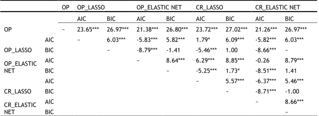
2.5 Empirical results ... 34 2.5.1 Accuracy ... 34 2.5.2 Statistical significance ... 36 2.5.3 Robustness tests ... 37 2.5.4 Discussion ... 44 2.6 Conclusion ... 45 References ... 47 Appendix ... 52
Chapter 3 What influences a bank’s decision to go public?... 68
Abstract ... 68
3.1 Introduction ... 69
3.2 Literature ... 71
3.3 Data and summary statistics ... 78
3.3.1 Data description ... 78
3.3.2 Choice of explanatory variables... 79
3.3.3 Summary statistics ... 79
3.4.1 Cox proportional hazard model (CPH) ... 82
3.4.2 Discrete hazard model (DH) ... 83
3.4.3 Logistic model ... 83
3.4.4 LASSO ... 83
3.4.5 L1 Penalized Semi-Parametric Cox Proportional Hazard Model (Penalized CPH model) ... 85
3.4.6 L1 Penalized Discrete Hazard Model (Penalized DH model) ... 85
3.4.7 L1 Penalized Logistic Model (Penalized Logistic Model) ... 86
3.5 Predictive ability ... 87
3.5.1 CPH and penalized CPH ... 87
3.5.2 Predictive Deciles ... 88
3.6 An empirical application using US data ... 89
3.6.1 The pre-crisis period ... 90
3.6.2 The crisis period ... 93
3.6.3 The post-crisis period ... 96
3.7 Conclusion ... 98
References ... 99
Appendix ... 104
Chapter 4 Predicting failure: evidence from UK firms ... 109
Abstract ... 109
4.1 Introduction ... 110
4.2 Literature ... 113
4.3 Data and summary statistics ... 119
4.3.1 Data sources ... 119
4.3.2 Choice of explanatory variables... 121
4.3.3 Summary statistics ... 124
4.4 Methodology ... 127
4.4.1 Discrete Hazard (DH) model ... 127
4.4.2 The Bayesian Model Averaging (BMA) version of DH models ... 129
4.4.3 Naive Bayes (NB) Classifier ... 133
4.4.4 K-nearest neighbours (k-NN) classifier ... 135
4.5 Empirical results ... 136
4.5.1 Whole period (1991-2009) ... 137
4.5.2 The sub-sample periods ... 140
4.5.3 The sub-samples in cross sections ... 147
4.6 Conclusion ... 154
References ... 156
List of Tables
Table 2-1 Rating categories ... 19
Table 2-2 CDSIRs of firms by year ... 23
Table 2-3 EQIRs of firms by year ... 23
Table 2-4 Descriptive statistics-CDSIRs ... 24
Table 2-5 Descriptive statistics-EQIRs ... 26
Table 2-6 Accuracy Ratios and selected variables ... 35
Table 2-7 Accuracy Ratios and selected variables (10-fold cross validation) ... 38
Table 2-8 PCA combined with OP ... 39
Table 2-9 Accuracy Ratios and selected variables (scaled LASSO) ... 40
Table 2-10 CP Ratios and selected variables ... 41
Table 2-11 Equal performance tests of out-of-sample prediction of CDSIRs ... 42
Table 2-12 Equal performance tests of out-of-sample prediction of EQIRs ... 42
Table 2-13 Accuracy Ratios and selected variables (investment-grade ratings) . 43 Table 2-14 Accuracy Ratios and selected variables (random effects) ... 44
Table 3-1 The distribution of banks ... 78
Table 3-2 Summary statistics ... 81
Table 3-3 Accuracy ratios and the number of surviving variables in the CPH model and its penalized versions ... 87
Table 3-4 IPO decision by out-of-sample prediction decile ... 89
Table 3-5 The estimates of candidate models in the pre-crisis period ... 91
Table 3-6 The estimates of candidate models in the crisis period ... 94
Table 3-7 The estimates of candidate models in the post-crisis period ... 96
Table 4-1 Expected signs and variables definition... 122
Table 4-2 Firms by year ... 124
Table 4-3 Descriptive statistics ... 126
Table 4-4 Sample means ... 127
Table 4-5 AUC and brier scores for all competing models during 1991-2009 .... 138
Table 4-6 Defaults by out-of-sample prediction decile among model related to the DH model during 1991-2009 ... 140
Table 4-7 Defaults by out-of-sample prediction decile in the NB classifier and the k-NN classifier during 1991-2009 ... 140
Table 4-8 AUC and brier scores for all competing models during 1994-2009 .... 141
Table 4-9 Defaults by out-of-sample prediction decile among model related to the DH model during 1994-2009 ... 141
Table 4-10 Defaults by out-of-sample prediction decile in the NB classifier and the k-NN classifier during 1994-2009 ... 142
Table 4-11 AUC and brier scores for all competing models during 1991-2007 ... 143
Table 4-12 Defaults by out-of-sample prediction decile among model related to the DH model during 1991-2007 ... 143
Table 4-13 Defaults by out-of-sample prediction decile in the NB classifier and the k-NN classifier during 1991-2007 ... 143
Table 4-14 AUC and brier scores for all competing models during 1994-2007 ... 145
Table 4-15 Defaults by out-of-sample prediction decile among model related to the DH model during 1994-2007 ... 145
Table 4-16 Defaults by out-of-sample prediction decile in the NB classifier and the k-NN classifier during 1994-2007 ... 145
Table 4-17 AUC and brier scores for all competing models during 1991-2009_small firms ... 148
Table 4-18 Defaults by out-of-sample prediction decile among model related to the DH model during 1991-2009_small firms ... 148
Table 4-19 Defaults by out-of-sample prediction decile in the NB classifier and the k-NN classifier during 1991-2009_small firms ... 148 Table 4-20 AUC and brier scores for all competing models during 1991-2009_large firms ... 149 Table 4-21 Defaults by out-of-sample prediction decile among model related to the DH model during 1991-2009_large firms ... 150 Table 4-22 Defaults by out-of-sample prediction decile in the NB classifier and the k-NN classifier during 1991-2009_large firms ... 150 Table 4-23 AUC and brier scores for all competing models during
1991-2009_young firms ... 151 Table 4-24 Defaults by out-of-sample prediction decile among model related to the DH model during 1991-2009_young firms ... 151 Table 4-25 Defaults by out-of-sample prediction decile in the NB classifier and the k-NN classifier during 1991-2009_young firms ... 151 Table 4-26 AUC and brier scores for all competing models during 1991-2009_old firms ... 152 Table 4-27 Defaults by out-of-sample prediction decile among model related to the DH model during 1991-2009_old firms ... 152 Table 4-28 Defaults by out-of-sample prediction decile in the NB classifier and the k-NN classifier during 1991-2009_old firms ... 153
Acknowledgements
I would like to express my deepest gratitude to my principal supervisor Professor Serafeim Tsoukas. Without his continuous faith, encouragement and academic support, I would have had difficulty starting a PhD, let alone completing it. He is a dedicated mentor and I am also thankful for all the wonderful opportunities in academia he has given me. The PhD has been an unforgettable experience. Similarly, my profound thanks go to my second supervisor Professor Georgios Sermpinis for his guidance and support. I am deeply appreciative all discussions with him, which gave me valuable suggestions for my work. It will keep fond memories of my PhD time.
I am also appreciative to the editors and anonymous referees of the Journal of Empirical Finance for their comments and suggestions, which have greatly helped to improve my research. Additionally, I acknowledge the financial support provided by the China Scholarship Council (CSC) and the academic environment created by staff at the Adam Smith Business School.
Special mentions go to my friends and colleagues. In particular, I extend thanks to Li Pan and Jingxuan Zhang for all the experiences we have had together. Last but not least, I am greatly indebted to my mum, dad and younger brother. Without their inspiration, love and support, I would not be the person I am today. My every success belongs to them as well.
Author’s Declaration
I declare that, except where explicit reference is made to the contribution of others, that this dissertation is the result of my own work and has not been submitted for any other degree at the University of Glasgow or any other institution.
Printed Name: Ping Zhang
Chapter 1
Introduction
1.1
General background
Financial forecasting has significant ability to influence future activities for market participants. Providing accurate forecasts generally helps market participants to reduce uncertainty around costs, identify market tendencies, and manage efficient plans, which can frequently be achieved by statistical models in financial research. Such models can be explanatory or predictive, and serve to evaluate and develop theories in terms of causality or prediction (Shmueli 2010). Compared with explanatory models, predictive models have some attractive characteristics (Shmueli and Koppius 2011). First, more underlying patterns and relationships in a large, complex dataset can be captured by predictive analytics, and hence new causality would be suggested. As data storage and computing techniques advance, many individuals can be recorded and the substantial features of each individual can be tracked simultaneously in the dataset (Giraud 2015). Thus, an extensive set of potential variables capturing diverse economic theories can be extracted from the dataset and applied to building a model. Predictive models are able to reduce the interference from superabundant outliers in the dataset and simplify the constructed model. Moreover, predictive models can evaluate the predictive ability of predictors with high explanatory ability. Finally, more accurate forecasts can be provided by predictive models. In this thesis, we focus on exploring the properties of predictive models in empirical analysis to clarify important predictors and produce more accurate prediction for specific financial outcomes.
Considering bias-variance trade-off, two types of techniques are developed to provide more accurate forecasts and a sparser representation in predictive models (Shmueli and Koppius 2011). The first is called the shrinkage approach, which contains principal components regression, ridge regression and its extensions and so on. In this approach the bias is allowed, and the variance is reduced, and the major patterns are therefore captured to produce improved prediction. The second is related to ensemble technique in machine learning, for example bagging (Breiman 1996), boosting (Schapire 1999) and Bayesian derivatives. This method tends to combine several predictions from different models to generate more accurate prediction. We choose in particular in this thesis two variable selection
techniques from these predictive models, where the least absolute shrinkage and selection operator (LASSO) is related to shrinkage approach and Bayesian model averaging (BMA) is derived from Bayesian theory.
The least absolute shrinkage and selection operator (LASSO), developed by Tibshirani (1996), can be regarded as a hybrid of variable selection and shrinkage estimators. It enables estimation and variable selection simultaneously in the non-orthogonal setting. If the tuning parameter exceeds a threshold value in LASSO, the coefficients of non-relevant independent variables are forced to zero in the model and the less shrinkage is allowed to be placed on the important predictors. Therefore, the multi-collinearity problem can be solved, and a more interpretable and sparser model can be generated after the LASSO estimator. Moreover, due to the smooth form of the penalty function, LASSO can select fewer independent variables and is a more stable model in comparison with best-subset and stepwise selection methods. Since LASSO can successfully be applied with an extensive set of predictors, the outstanding flexibility of LASSO can adjust to any changes to variables in the application. In addition, due to the exclusion of interfering information, the predictive performance will be better than in the conventional models.
Before LASSO was developed, best-subset (Hocking and Leslie 1967) and stepwise selection (Draper and Smith 1966) methods as representatives of variable selection techniques in predictive models were developed in the 1960s and generally implemented into scientific research due to their simple application and ease of interpretation. However, these methods have some disadvantages compared with LASSO. Tibshirani (1996) and Zou (2006) demonstrate that subset variable selection is not stable during the discrete process, even if the dataset changes slightly. When potential independent variables are large, the computation of subset selection is complex, which is always substituted by the stepwise subset selection (Tian et al. 2015). Fan and Li (2001) further mention that stochastic errors are omitted, and estimation is biased in the application of stepwise selection, since it is just based on correlation between latent variables.
Moving to the other type of variable selection techniques in this thesis, Bayesian Model Averaging (BMA) is one part of the averaging approach, which is extended from the usual Bayesian inference methods. It captures parameter uncertainty in
Chapter 1 1.2 Structure
one model through the prior distribution and solves model uncertainty by posterior parameter using Bayes’ theorem (Fragoso et al. 2018). It should be noted that variable selection procedure in BMA is entirely different from LASSO. If researchers focus on variable or model selection, the variable or model with the highest posterior probability will be chosen and then this will be used to generate predictions. This compromise between selection and prediction can be easily completed by the Stochastic Search Variable Selection (SSVS) (Lamon and Clyde 2000) or the Reversible Jump Markov Chain Monte Carlo (RJMCMC) algorithm (Jacobson and Karlsson 2004). In other words, it allows for direct model selection, combined estimation and prediction together, and further suggests that parameter and model uncertainty are taken into account in inferences and predictions. Considering the model evaluation, Madigan and Raftery (1994) confirm that the BMA approach can produce predictions with lower risk under a logarithmic scoring rule than using a single model.
In this thesis, we aim to apply these variable selection techniques to determine and forecast some corporate events such as Market Implied Ratings (MIRs), Initial Public Offering (IPO) decisions and the failure of a firm. It is known that even financial analysts or outsider investors cannot get the full information about companies from published information. This implies that these market participants are likely to miss investment chances or take more credit risks in the financial market. To reduce these risks and assess a company from various points of view, specific events in a firm’s life (such as equity or debt issuance) are now considered as the primary signal of the firm’s operating information available to outsiders (Sena 2002). An increasing number of researchers have emphasised specific corporate events to evaluate the financial health of companies (Eckbo 2009).
1.2
Structure
In order to better organize this thesis, we divide the systematically empirical forecast exercise into three main chapters. In Chapter 21, we investigate the determinants of market implied ratings (MIRs) in relation to firm-specific factors,
1 This chapter is based on a research paper co-authored with my supervisors Serafeim Tsoukas and Georgios Sermpinis, where is published on Journal of Empirical Finance.
market-driven indicators and macroeconomic predictors, and then forecast them. Graham and Harvey (2001) demonstrate that credit ratings have considerable influence on debt issuance and capital structure. Making accurate predictions of corporate credit ratings is a crucial issue to both investors and rating agencies. Compared with conventional long-term credit ratings, MIRs can be published with high frequency, incorporating market information into data-intensive rating models, which provide more timely information about credit quality at short and medium term horizons (Rösch 2005, Tsoukas and Spaliara 2014). Hence, we employ the literature of credit ratings as foundations to evaluate the predictive performance of all candidate models that capture volatile market changes. Since MIRs are assigned into ordinal categories, ordered probit models are applied as the benchmark to define and forecast MIRs (Pasiouras et al. 2006, Hwang et al. 2010, Mizen and Tsoukas 2012, Hwang 2013). The variable selection technique (LASSO) and its extension (the Elastic net) are then added into the ordered probit model and continuation ratio model to determine and forecast MIRs.
From the conclusions of Chapter 2, we first indicate that MIRs can be affected by several firm-specific, market-driven and macroeconomic variables. Meanwhile, we confirm LASSO models can provide better predictive performance on the out-of-sample MIRs than the ordered probit model and simultaneously the most important predictors can be selected in LASSO models. We also demonstrate that the more accurate out-of-sample prediction and fewer predictors can be produced in the LASSO models with BIC-type tuning parameter selector than their LASSO counterparts with AIC-type selector. To validate our results, different robustness tests are applied, and our main results are robust to the above modifications. Thus, LASSO-selected models provide better predictive performance in ordinal financial outcomes.
In Chapter 3, a bank’s IPO decision is chosen as a targeted event for empirical investigation. A bank is a financial intermediary whose core activity is to provide loans to borrowers and collect deposits from savers. The operating status of a bank is associated with the allocation of financial resources and the growth of investment in financial markets, which influence the cost of financial intermediation and the stability of the whole financial market. Since equity finance in the USA has become an important source of funding for banks, a bank’s decision to go public has been attracting more attention from academics. We
Chapter 1 1.2 Structure
apply accounting ratios and other publicly available information in Cox proportional hazard model and its penalized model to identify the factors that influence a bank’s IPO decision and predict the IPO decision. Since our dataset extends from 1996 to 2016, covering the key years of the banking crisis (2007-2009), we separate the dataset into pre-crisis, crisis and post-crisis periods and assess how market conditions influence the probability of banks going public. According to the results, we first document that selected variables are indicators affecting the probability of a bank’s IPO decision and further detect that a bank’s IPO decision is more sensitive to the change in its financial health in extreme economic events than in non-crisis periods. Moving to the analysis of predictive performance, we observe a significant increase in the percentage of correct out-of-sample forecasts of IPO decisions for banks by adding the LASSO estimator into the Cox proportional hazard model. On the other hand, we indicate that the Cox proportional hazard model underperforms discrete hazard and logistic models and the Cox model with LASSO estimator outperforms discrete hazard, logistic models and their LASSO version. This highlights the effect of LASSO on our algorithms. In line with the conclusion in Chapter 2, the LASSO models controlled by BIC-type tuning parameter selector can provide a sparser model and higher predictive power in out-of-sample forecasts than their counterpart with AIC-type selector. Both Chapters 2 and 3 confirm that the LASSO technique can identify the most relevant predictors from an extensive set of candidate variables without considering a pre-selection of these potential variables (van de Geer 2008), enhance the predictive ability (Fan and Li 2001, Tian et al. 2015) and sidestep the problem of multi-collinearity (Tibshirani 1996).
Next, in Chapter 4 we forecast the failure of private firms by firm-specific and macroeconomic indicators in the UK. The UK as a developed European country entered into economic recession from 2008 with the signal that the real Gross Domestic Product (GDP) growth rate was extremely low. According to the US market performance after the financial crisis, increased credit risk for UK firms can be supposed. Therefore, providing precise forecasts of UK firms’ failure is necessary for their managers, potential investors or policy makers, helping them reduce the probability of being exposed to credit risk and preventing economic depression. To distinguish this work from the literature, we choose private firms with small and medium-scale operating in several industries in the UK, because
the growth of these firms has become the main power in economic development (Beck et al. 2005). The data period from 1991 to 2009 covers two important financial crises in UK economic history: the 1991–1993 European Exchange Rate Mechanism (ERM) currency crisis and the 2008-2009 global financial crisis (GFC). This provides an opportunity for us to detect whether the predictive powers of all candidate models are sensitive to financial crises. Meanwhile, we divide our dataset into two cross-sections, to capture two dimensions of firm heterogeneity (size and age). This could help us detect whether the cross-sectional differences affect the predictive ability of each model. To evaluate the predictive ability, we apply a combined model by discrete hazard model and BMA model to solve the parameter and model uncertainty and assess the predictive performance of firms’ failure compared with the discrete hazard model and traditional classifiers, the Naive Bayes (NB) classifier and the k-nearest neighbours (k-NN) classifier.
From the main conclusions, the top two models providing higher predictive ability in firms’ failure are the BMA of discrete hazard models and the NB classifier. The NB classifier outperforms the BMA version of discrete hazard model in some sub-samples while the predictive ability of the BMA version of discrete hazard model is comparable with that of the NB classifier. It should be noted that adding BMA into the discrete hazard models can increase the predictive accuracy in out-of-sample prediction and solve parameter and model uncertainty. The results also suggest that financial crisis and firm heterogeneity can affect the predictive power of each candidate model. We also observe that considering time effects or industry effects can improve the accuracy of out-of-sample prediction in different periods, especially for discrete hazard model and its BMA version.
In the last chapter, we conclude all empirical work and suggest some topics for future research.
Chapter 1 References
References
Beck, T., Demirguc-Kunt, A. and Levine, R. (2005) 'SMEs, Growth, and Poverty: Cross-Country Evidence', Journal of Economic Growth, 10(3), 199-229.
Breiman, L. (1996) 'Bagging Predictors', Machine Learning, 24(2), 123-140.
Draper, N. R. and Smith, H. (1966) Applied Regression Analysis, New York: John Wiley & Sons.
Eckbo, B. E. (2009) Handbook of Corporate Finance: Empirical Corporate Finance. Vol. 1,
Amsterdam: Elsevier North-Holland.
Fan, J. and Li, R. (2001) 'Variable Selection via Nonconcave Penalized Likelihood and Its Oracle Properties', Journal of the American Statistical Association, 96(456), 1348-1360.
Fragoso, T. M., Bertoli, W. and Louzada, F. (2018) 'Bayesian Model Averaging: A Systematic Review and Conceptual Classification: BMA: A Systematic Review', International Statistical Review, 86(1), 1-28.
Giraud, C. (2015) High-dimensional Statistics, Boca Raton: CRC Press.
Graham, J. R. and Harvey, C. R. (2001) 'The Theory and Practice of Corporate Finance: Evidence from the Field', Journal of Financial Economics, 60(2), 187-243.
Hocking, R. R. and Leslie, R. N. (1967) 'Selection of the Best Subset in Regression Analysis',
Technometrics, 9(4), 531-540.
Hwang, R.-C., Chung, H. and Chu, C. K. (2010) 'Predicting Issuer Credit Ratings Using a Semiparametric Method', Journal of Empirical Finance, 17(1), 120-137.
Hwang, R. C. (2013) 'Forecasting Credit Ratings with the Varying-Coefficient Model', Quantitative Finance, 13(12), 1947-1965.
Jacobson, T. and Karlsson, S. (2004) 'Finding Good Predictors for Inflation: A Bayesian Model Averaging Approach', Journal of Forecasting, 23(7), 479-496.
Lamon, E. C. and Clyde, M. A. (2000) 'Accounting for Model Uncertainty in Prediction of Chlorophyll in Lake Okeechobee', Journal of Agricultural, Biological, and Environmental Statistics, 5(3), 297-322.
Mizen, P. and Tsoukas, S. (2012) 'Forecasting US Bond Default Ratings Allowing for Previous and Initial State Dependence in an Ordered Probit Model', International Journal of Forecasting,
28(1), 273-287.
Pasiouras, F., Gaganis, C. and Zopounidis, C. (2006) 'The Impact of Bank Regulations,
Supervision, Market Structure, and Bank Characteristics on Individual Bank Ratings: A Cross-Country Analysis', Review of Quantitative Finance and Accounting, 27(4), 403-438.
Rösch, D. (2005) 'An Empirical Comparison of Default Risk Forecasts from Alternative Credit Rating Philosophies', International Journal of Forecasting, 21(1), 37-51.
Schapire, R. E. (1999) 'A Brief Introduction to Boosting', in Proceedings of the 16th international joint conference on Artificial intelligence - Volume 2, Stockholm, Sweden, 1624417: Morgan Kaufmann Publishers Inc., 1401-1406.
Sena, V. (2002) 'Empirical Corporate Finance: Volumes I, II, III and IV. Edited by Brennan (Michael J.)', 112(Generic), F358-F360.
Shmueli, G. (2010) 'To Explain or to Predict?', Statistical Science, 25(3), 289-310.
Shmueli, G. and Koppius, O. R. (2011) 'Predictive Analytics in Information Systems Research', MIS Quarterly, 35(3), 553-572.
Tian, S., Yu, Y. and Guo, H. (2015) 'Variable Selection and Corporate Bankruptcy Forecasts',
Journal of Banking and Finance, 52, 89-100.
Tibshirani, R. (1996) 'Regression Shrinkage and Selection via the Lasso', Journal of the Royal Statistical Society. Series B (Methodological), 58(1), 267-288.
Tsoukas, S. and Spaliara, M.-E. (2014) 'Market Implied Ratings and Financing Constraints: Evidence from US Firms: Market Implied Ratings and Financing Constraints', Journal of Business Finance & Accounting, 41(1-2), 242-269.
van de Geer, S. A. (2008) 'High-Dimensional Generalized Linear Models and the Lasso', The Annals of Statistics, 36(6), 614.
Zou, H. (2006) 'The Adaptive Lasso and Its Oracle Properties', Journal of the American Statistical Association, 101(476), 1418-1429.
Chapter 2
Modelling market implied ratings
using LASSO variable selection techniques
Abstract
Both investors and rating agencies are interested in the accurate forecasting of corporate credit ratings to manage credit risk. In this chapter, financial factors, market-driven indicators and macroeconomic predictors are applied to determine market implied credit ratings. Adding a variable selection technique, the least absolute shrinkage and selection operator (LASSO) into reduced-form models can significantly improve predictive power. Moreover, when we compare our LASSO models with the benchmark ordered probit model, it can be shown that the former models have superior predictive ability and outperform the latter model in all out-of-sample predictions.
2.1
Introduction
Credit ratings are regarded as a measurement of the creditworthiness of a firm, and they are widely used to quantify the credit risk for the firm’s external investors. They show the likelihood that a given borrower will default. They are generally issued by rating agencies such as Standard and Poor’s, Moody’s and Fitch according to the assessment of a firm’s ability and willingness to fulfil debt servicing obligations in a specific period. This ability has significant potential to affect the pricing of credit risk and the allocation of investment strategies. According to the Financial Crisis Inquiry (2011), credit rating agencies as a key factor added to the most recent financial crisis in the US, since the updating of ratings was unable to adjust quickly to market changes. The users of credit ratings blindly rely on these ratings as early warning signals to identify credit risks in financial markets, which become the other element of this financial turmoil. Hence, rating accuracy and the process by which firms are assigned their ratings have been widely contested in the US. Fitch has recently developed a new model to derive Market Implied Ratings (MIRs) from bond and equity prices. The appealing advantage of these ratings in comparison with the conventional agency ratings is that they adjust instantaneously to market changes.
In this chapter, we aim to develop methodological extensions by adding a variable selection approach, the least absolute shrinkage and selection operator (LASSO), and its most promising derivation, the Elastic net, to ordered probit and continuation ratio models. The task in hand involves forecasting Fitch’s CDS and Equity implied ratings (CDSIRs and EQIRs respectively hereafter). The major research contribution is to exploit LASSO properties and define the underlying structure of CDSIRs and EQIRs.1 Firm-specific ratios from accounting reports and other publicly available information have been implemented in previous studies to predict credit ratings. The most important determinants for predicting bond ratings are identified by various techniques (OLS, multinomial and ordered logit/probit models) in this work (see for instance the early studies by Pogue and Soldofsky 1969, Pinches and Mingo 1973, Kaplan and Urwitz 1979, Kao and Wu 1990). The results suggest that a firm’s financial situation and the economic
1 With respect to the latter aim of this study, for reasons of space we do not report estimated coefficients of the prediction models. These results are available upon request.
Chapter 2 2.1 Introduction
environment can influence its ratings and the forecasting of default. Mizen and Tsoukas (2012) confirm the importance of capturing dynamic settings in ratings during model estimation and demonstrate that controlling state dependence can increase the percentage of correct prediction by the models.
In another line of credit ratings research, an increasing number of applied rating predictors as input in a model can be observed in literature, since researchers tend to capture more economic theories to define or forecast ratings. This gives us the opportunity to ask whether the predictors used are relevant in a piece of work. On the one hand, if only the subset of applied factors is related to ratings, it means that potentially important determinants of ratings are omitted, leading to a decrease in prediction accuracy. On the other hand, when the extensive set of predictors can explain rating, the multi-collinearity problem is likely to be met, resulting in biased estimation. If the multi-collinearity problem is not at work, a sparse representation cannot be provided due to a large number of applied predictors, which means that these models cannot be easily explained and readily used by market participants and rating agencies.
Our methodology carefully follows the literature that examines the determinants of credit ratings, but we add to it in two important ways. First, a methodological contribution is made by deriving a simple and more intuitive, yet innovative model, which is based on the variable selection technique, developed by Tibshirani (1996)—the least absolute shrinkage and selection operator (LASSO). Fan and Li (2001) and Tian et al. (2015) indicate that the most important predictors can be automatically selected from an extensive set of candidate variables and the predictive performance can simultaneously be improved in LASSO. Furthermore, LASSO does not depend on strict presumptions such as a pre-selection of the variables considered, and it is statistically consistent even under infinity observations (van de Geer 2008). It should be noted that LASSO can solve the problem of multi-collinearity that is fairly common in probit/logit models. In addition, LASSO technique is computationally efficient even when a large set of potential predictors are used. Our study is the first to provide a systematic empirical analysis of LASSO techniques in MIRs forecasts. In doing so, we investigate the relative importance of several time-varying covariates from an extensive set of firm-specific factors, market-specific predictors and macro-economic indicators applied to predict market implied ratings. After model
estimation, a parsimonious set of predictors will be produced which can be readily employed by investors, managers and credit risk agencies.
Second, our panel dataset is constructed by market implied ratings instead of the standard long-term ratings. Compared with long-term ratings, MIRs represent an innovation to the ratings industry to address the issue of staleness in their long-term counterparts. Rösch (2005) and Tsoukas and Spaliara (2014) state that MIRs depend on proprietary and data-intensive rating models that incorporate market information into a model-based credit assessment. The most attractive characteristic of these ratings is that they can adjust immediately to market changes. Hence, we build on the foundations of the literature on implied ratings by investigating the forecasting power of models that capture volatile market changes.
To preview our findings, market implied ratings can be explained by several financial factors along with market-driven and macroeconomic indicators. Importantly, applying the LASSO techniques can considerably enhance the predictive power of our models in out-of-sample predictions compared to the benchmark (ordered probit model) which is commonly adopted in the literature. Moreover, the predictive performance of the LASSO models controlled by BIC-type tuning parameter selector are superior to their LASSO counterparts with AIC-type selector for the dataset and periods under our study. Thus, we suggest that LASSO-selected models can be implemented in future research to produce improved rating prediction.
The rest of the chapter is structured as follows. The literature of forecasting credit ratings and variable selection techniques is presented in section 2. We discuss the data and summary statistics in section 3. Following that, we describe our methodology in section 4. The empirical results and robustness tests are reported in section 5. The main conclusion is demonstrated in the final section.
2.2
Literature
The ways in which rating agencies use public information in setting quality ratings and researchers provide accurate prediction of ratings in the literature are contentious issues. Verifying the categories of credit ratings of companies is the
Chapter 2 2.2 Literature
extended work of identifying the default probabilities of companies in credit risk management. Horrigan (1966) first introduced the work of predicting bond ratings through accounting data and financial ratios from balance sheets and subordination. To provide a better set of financial ratios explaining credit ratings, Horrigan tested different combinations of predictor and kept the best one with the highest value of R-squared. This set was constructed by total assets, net worth to the book value of total debt, net operating profit to sales, working capital to sales adjusted industrial effects, and sales to net worth adjusted industrial effects. A dummy variable represented the subordination status of bond ratings, which produces about 60% correct out-of-sample prediction of newly issued and changed ratings. Unlike Horrigan's study (1966), Pogue and Soldofsky (1969) estimated the conditional probability that a bond would be assigned the higher rating by employing financial ratios and then converted the estimated probability into different rating categories to assess the predictive performance. In their conclusion, they demonstrate that leverage, the variation of earnings, the size of firm and profitability can influence bond ratings. Since bond ratings are related to the default risk, West (1970) adopted the four components of risk premiums (earnings volatility, capital structure, reliability and marketability) from Fisher's study (1959) into Horrigan’s study to predict bond ratings again. He showed that the predictive accuracy of the Fisher model is higher than that of Horrigan’s model.
With the development of econometrics, some researchers emphasised using multiple discriminant analysis (MDA) to categorize bonds into different rating levels. Based on the theory of MDA, there is no need to transform ordinal data into interval scale since the analysis of MDA focuses on differences in each category in dependent variables. In other words, MDA ignores the ordinal properties of ratings and just regards different rating categories as various segmentations of a single risk dimension. Pinches and Mingo (1973) implemented two methodological steps to categorize the ratings of bond issues. The factor analysis was used first to identify relatively important predictors and then these predictors were employed in multiple discriminant analysis to evaluate newly issued bond ratings. They concluded that about 70% correct predictions in actual ratings can be observed and around 60% correct forecasts in newly issued bonds. To find more potential relationships between credit ratings and financial ratios,
Altman and Katz (1976) included 30 independent variables in MDA to determine the bond ratings of electric firms and confirmed that 14 predictors survived in the model and the predictive power in out-of-sample dataset increased to around 75%. Ang and Patel (1975) compared the predictive performance of methodologies applied in the studies of Horrigan (1966), Pogue and Soldofsky (1969), West (1970) and Pinches and Mingo (1973) in bond ratings. They confirmed that these models could be used in the prediction of short-term financial loss probability but they did not perform well in long-term prediction.
McKelvey and Zavoina (1975) developed a model known as the ordered probit model, for ordinal dependent variables, which assumed that the unobserved dependent variables were on an interval scale that could be measured by a linear model. They then divided these dependent variables with different cut-points to detect the ordinal dependent variable. This model provided a new opportunity for researchers to determine the ordinal ranks of credit ratings, and it is frequently used as a benchmark model to analyse credit ratings. Kaplan and Urwitz (1979) argued the disadvantages of using OLS and MDA models for analysing bond ratings and then implemented the probit models to estimate bond ratings. They point out that the results of financial ratios are similar to the conclusions reached by Pinches and Mingo (1973) and the market beta is one determinant of ratings. The predictive ability of the probit model is not significantly different from previous studies. Ederington (1985) further compared the application of four models on bond ratings, which contained a linear regression model, an ordered probit model, a linear discriminant model and a multinomial logit model. He confirmed that the ordered probit model clearly outperformed the regression model and the unordered logit model clearly dominated the discriminant model. Gentry et al. (1988) confirmed the predictive power of cash flow ratios during bond ratings categorization by using the probit model and suggested that involved inventories, other current liabilities, dividends, long-term financing and fixed coverage charges should be considered in the future prediction of bond ratings.
Previous research frequently emphasised analysing credit ratings under the assumption that rating standards are consistent. With an increasing number of downgrades in bond ratings, the performance of the debt market is gradually attracting researchers’ attention. Blume et al. (1998) tried to confirm whether the credit quality of corporate debt had worsened over time. They used
three-Chapter 2 2.2 Literature
year averages of financial ratios in an ordered probit model and detected that rating standards had become stricter. In this situation, they reported that firms were less likely to be assigned higher ratings levels in the mid-1980s and early 1990s. Following the variable selection criterion in the work of Blume et al. (1998), Poon (2003) constructed the global sample dataset by averaging three-year financial ratios and then applying the ordered probit model to detect the indicators of credit ratings. He demonstrated that a government’s credit risk is an important determinant of long-term ratings and it has a positive relationship with long-term ratings.
From the abovementioned literature, it can be seen that different statistical models capturing the characteristics of a dataset provide various ratings predictions and researchers cannot successfully suggest a preferred model. Kamstra et al. (2001) applied ordered logit regression (similar to the ordered probit model) combining methods to improve the predictive accuracy of bond ratings in the transportation and industrial sectors and confirmed that combined forecasts outperform their input forecasts. More recently, ordered probit methodologies have been commonly applied by for instance Amato and Furfine (2004) Hwang et al. (2009) and Hwang et al. (2010) to forecast credit ratings. Amato and Furfine (2004) confirmed that credit ratings change based on the state of the business cycle, by analysing US firms in the ordered probit model. Moreover, they demonstrated procyclicality in the ratings of investment grade firms or newly assigned firms. Hwang et al. (2009) documented an analysis on the S&P’s long-term issuer credit rating. They used a stepwise selection model on 24 latent independent variables to select relatively important ones before applying a mollified ordered probit model. In particular, there were two market-driven variables, three accounting variables and industry effect variables in the final list of independent variables. The estimated coefficients of final predictors met expectations. The predictive accuracy of long-term ratings can reach up to around 72.84% and 77.16% using different cut-off values in the ordered probit model. Hwang et al. (2010) constructed a prediction model by changing the linear regression function in the common ordered probit model into a semiparametric function and confirmed this developed model can outperform the original one in out-of-sample prediction. It was identified in both studies that some indicators
are essential in forecasting credit ratings, such as the size of the company, balance sheet position, stock market performance and industry effects.
Altman and Kao (1992) report strong evidence that there was some serial correlation of ratings changes if the primary change was a downgrade, but no autocorrelation when the primary change was an upgrade, according to the two time periods examined, from 1970 to 1979, and from 1980 to 1985. As previously indicated, the balance sheet always shows the performance of a firm in a specific previous time period. This means that current credit ratings may be related to previous credit ratings and other previous accounting information about the corresponding firm. Parnes (2007) confirmed this changing tendency using several nonlinear models, which illustrate a clear positive autocorrelation among downgrade probabilities. By using the internal correlations model he also showed that time-series fluctuation is a more significant property in credit ratings than cross-ratings correlations.
Hwang (2013b) considered the autocorrelation of credit ratings in the dynamic ordered probit model (DOPM). In the empirical results, the out-of-sample total error rate was smaller and there was lower volatility compared with the simple DOPM under independence assumption. Hwang (2013a) further modified the DOPM by using smooth functions of macroeconomic variables to represent coefficients of firm-level independent variables in the DOPM, which is called the dynamic ordered varying-coefficient probit model (DOVPM). The latent coefficient functions in DOVPM can be measured by applying a local maximum likelihood method. The conclusion of this paper illustrated that the macroeconomic situation definitely influences the changing tendency of firm-level predictors. At the same time, the performance of DOVPM is obviously better than DOPM when it comes to predictive accuracy and total error rates of the prediction in the out-of-sample dataset. Both studies provide evidence that capturing the dynamic features of long-term ratings can increase predictive accuracy (see Hwang 2013b, Hwang 2013a). This conclusion is further supported by Mizen and Tsoukas (2012), who documented that the predictive performance in long-term ratings can be improved by considering the persistence of ratings. Tsoukas and Spaliara (2014) attempted to discover the relation between market implied ratings and financial constraints by adopting the ordered probit model. Their conclusion was that financial ratios are critical in ratings forecasts if a firm is likely to encounter financial difficulties.
Chapter 2 2.2 Literature
Moving to the literature of implied ratings, almost all studies focus on detecting the differences between long-term agency ratings and market implied ratings. Breger et al. (2003) indicated that bond spreads have explanatory ability to define the cut-off points of categorized bonds and suggested that implied ratings perform better in identifying default probability compared with other ratings. After that, Rösch (2005) confirmed this finding and demonstrated that the default probability can be appropriately reflected by implied ratings in comparison with standard ratings. Castellano and Giacometti (2012) observed that the changes in credit ratings could be predicted by market implied ratings.
The variables selection techniques are not widely applied in determining or predicting credit ratings. Only a small amount of work can be found that studies bankruptcy. Amendola et al. (2012) first employed the LASSO approach to estimate the default probabilities of Italian companies in the limited liability sector. According to their conclusion, the LASSO approach can provide a superior predictive performance and more stable error rates than previous default models. Härdle and Prastyo (2013) aimed to forecast the default probability of Southeast Asian firms by adding LASSO and elastic net in the logit model and confirmed that adding these penalty functions into the model can clearly improve the predictive accuracy. To provide general evidence supporting the predictive ability of LASSO on default risk, Tian et al. (2015) studied a comprehensive U.S. bankruptcy database and concluded that accuracy in out-of-sample prediction is superior than in previous models (like reduced-form models with the distance to default) in estimating default by combining reduced model with the LASSO technique.
Importantly, the first study of LASSO was developed by Tibshirani (1996). He suggested two reasons why LASSO should be created on the basis of Ordinary Least Squares (OLS). First, OLS estimates have low bias but large variance. However, in LASSO, non-relevant variables in the regression would be forced to 0, which allows bias and reduces the variance of predicted value. It can improve the predictive power of OLS. The second reason is the power of interpretation. Faced with vast predictors in OLS estimates, there exist complex and important elements illustrating how predictors affect the dependent variable. In LASSO, due to zero coefficients of some predictors, the strongest effects can be determined objectively, which make the analysis more reasonable.
Zou and Hastie (2005) combined LASSO with ridge regression to produce the Elastic net, which is a good hybrid of sparsity and regulation. There exist some advantages of using the Elastic net. First, it can select correlated independent variables in the grouping effect. In addition, the penalty function is strictly convex, thus a unique global minimum would be calculated. Finally, it is useful to solve the problem that the number of predictors is bigger than the number of observations. Although the Elastic net is not very widely used in econometrics, it has been employed on microarray data and in gene selection.
From the above review, the determinants of credit ratings prediction are provided, which is helpful to identify relevant predictors in market implied ratings. Meanwhile, the development of econometric methods in credit ratings is shown, which gives us the opportunity to make a methodological contribution. We will discuss the applied dataset and estimation strategy in the following sections.
2.3
Data and summary statistics
2.3.1
Data sources
Fitch’s database is employed to extract the data on market implied ratings, which refers to solicited ratings for all traded companies in the US. This database provides information on the CDS and Equity implied ratings assigned to each issuer as well as the date that the rating became available. From 2002 to 2008, both CDS and Equity implied ratings are reported on a monthly basis.2 Following normal practice in the literature, we categorize our firms into rating buckets without consideration of notches (i.e. + or -). According to the studies of Amato and Furfine (2004) and Mizen and Tsoukas (2012), this classification considers large cumulative changes of ratings rather than small movements notch by notch and avoids very few observations in one rating category. Therefore, seven rating
2 The research aims to study the structure and predictability of the implied ratings in the years preceding the recent global financial crisis. Our choice to focus on a time window ending in 2008 is motivated by two important considerations. First, the global financial crisis and the collapse of Lehman Brothers constituted a shock that may have acted as a confusing factor in the determination of credit ratings. In fact, it can be argued that the misinterpretation of the credit ratings by investors was one of the main contributors to the crisis. Second, the data were downloaded early in 2010 from a research project supported by Fitch: the coverage period is therefore 2002-2008.
Chapter 2 2.3 Data and summary statistics
categories are created, ranging from AAA to Below CCC, which are assigned numerical values in Table 2-1, starting with 1 to AAA, 2 to AA…, 7 to Below CCC.3
Table 2-1 Rating categories
Market Implied Ratings Corresponding numerical values
AAA 1 AA 2 A 3 BBB 4 BB 5 B 6 Below CCC 7
Notes: The table presents the rating categories and the corresponding numerical values.
In our work, the independent variables can be divided into three parts: accounting variables, market-driven indicators and macroeconomic predictors. Firm-specific accounting data are taken from Fitch’s Peer Analysis Tool. Quarterly corporate historical data for all companies rated by Fitch can be accessed in this database. MIRs of firms are linked with Fitch’s balance sheet statements and profit and loss
accounts of corresponding firms. Hence, we merge the monthly MIRs data and quarterly firm-level accounting data to construct our dataset.4 For the final dataset, each firm with CDSIRs and EQIRs data and financial and market data can be observed every month. Following applied selection criteria in the literature, we keep companies with complete records on our explanatory variables and firm-months without negative sales and assets. To reduce the potential influence of outliers, the regression variables are winsorized at the 1st and 99th percentiles. Monthly data on market indicators and macroeconomic variables are downloaded from Bloomberg. Our combined sample ultimately comprises data for 211 firms operating in all sectors of the US economy except agriculture, forestry and fishing and public administration. The number of observations on each firm in this unbalanced panel vary between 1 and 63. Two features of our dataset make our
3 In EQIRs we do not observe any ratings in the last category, hence six groups are generated for this type of implied ratings.
4 For each firm, the quarterly data is repeated every month during the same quarter if the monthly data is not observed.
work attractive. First, both investment and speculative grades ratings are included in our dataset, which covers the whole spectrum of firms in line with previous studies (see for instance Amato and Furfine 2004). Second, there is no significant difference between the distribution of standard long-term ratings in CDS data and the distribution of agency ratings in the general bond population (see Reyngold et
al. 2007). Thus, our empirical analysis from both the CDSIRs and the EQIRs
databases has a representative base.
2.3.2
Choice of explanatory variables
Both business and financial risks are incorporated into previous empirical research to determine credit ratings. The business risk is a measure of industry characteristics, firm size, management capability and organizational indicators. Financial risk is related to the quality of a firm’s accounting procedures, profitability, cash flow situation and its overall financial policy. Market-related information is also considered in candidate models. Meanwhile, we check the material issued by rating agencies, especially Fitch, to verify what matters when assigning a market implied rating. In other words, the extensive selection of our explanatory variables is guided both from the existing empirical literature (see for example Kaplan and Urwitz 1979, Ederington 1985, Poon 2003, Chava and Jarrow 2004, Amendola et al. 2012, Mizen and Tsoukas 2012, Hwang 2013a, Creal et al. 2014, Doumpos et al. 2015, Tian et al. 2015), and the common practice of rating agencies (see Liu et al. 2007, Reyngold et al. 2007).5
2.3.2.1 Firm-specific variables
We apply 16 firm-specific accounting variables as potential predictors of ratings, which measure different aspects of firms’ financial health such as size, leverage, coverage, cash flow, profitability and liquidity. Specifically, the firm size (DETA) is calculated by the natural logarithm of firms’ real total assets, which indicates the scale of the firm. When firm size increases, the rating of the firm would be expected to improve. Next, we measure leverage using a number of ratios: The ratio of total assets over equity (AE), the ratio of long-term debt over total assets (LDA), the ratio of short-term debt to total assets (SDA), the ratio of total debt to
5 The expected relationship between these variables and MIRs is presented in Table A1 in Appendix A. The Table also provides a detailed description of the variables used in this study.
Chapter 2 2.3 Data and summary statistics
total assets (TDA), and the ratio of total debt to earnings before interest, taxes, depreciation, amortization, and restructuring or rent costs (TDEBITDA). The negative relationship between leverage and MIRs would be expected, since higher values for these ratios are likely to increase financial risk and hence should worsen the rating. The next two measures proxy the creditworthiness of the firm, as they show the firm’s ability to generate income to meet interest rate obligations: the ratio of earnings before interest and tax over interest expenses (EBITINT) and the ratio of earnings before interest, taxes, depreciation, amortization and restructuring or rent costs to interest expenses (EBITDAINT). If these ratios increase, this firm would have more ability to cover its obligations and reduce default risk, which would improve its rating. Further, cash flow is measured by the following ratios: cash flow from operating activities over total assets (CFOA), and cash and equivalent over total assets (CASHEQA). The positive relationship between these ratios and rating upgrades would be expected, since more cash flow would reduce liquidity risk and then improve ratings. The next five ratios explain the profitability of a firm: the ratio of operating income to net sales (OM), the ratio of net income without dividends over total capital (ROC), the ratio of net income over shareholders’ equity (ROE), the ratio of net income over total assets (ROA) and the ratio of the funds from operations to total debt (FFD). With the improvement in operation performance, more profitability should be expected, which implies an improvement of ratings. Finally, liquidity is expressed by the ratio of cash from operations to liabilities (LIQ), which shows the ability of a firm to satisfy its short-term obligations as they become due. A firm operating with higher levels of liquidity is likely to be assigned the higher-level rating.
2.3.2.2 Market-driven indicators
Since stock prices have the ability to reflect publicly available information, it is reasonable that market-driven variables can affect the rating of a company as indicated previously. Thus, we apply the following market indicators: excess return (EXRET) as calculated by the monthly stock return on a firm minus the S&P 500 index return and the relative size of a firm in the market (RSIZE) measured by each firm’s market equity value over the total market equity value. Both variables are expected to be positively associated with the improvement of ratings. Next, the volatility of stock return (STD) is expressed by the standard deviation of each company’s monthly stock returns. The systematic risk of each firm (BETA) is
employed, which is extracted from the Capital Asset Pricing Model for each firm. Finally, the 1-year and 5-year default probabilities (PD1 and PD5) are taken from Fitch’s Peer Analysis Tool. An increase in these variables indicates the growth of default probability, which would worsen ratings.
2.3.2.3 Macroeconomic influences
An extensive set of macro-economic variables as potential predictors is applied to determine market implied ratings. Specifically, returns on the S&P 500 index (RLSP) are calculated as the evaluation of the stock market performance. Short-term interest rates are measured by the three-month commercial paper rate (CPFFM), three-month Treasury bill rate minus federal funds rate (TB3) and the one-year constant maturity treasury rate (GS1). The general price level is employed, as measured by the growth rate in the narrow money stock (MB) and inflation rate (INFL). Aggregate economic activity is proxied by the rate of change in industrial production (DLIP), the index of the growth rate of real GDP (DLGDP), the average of monthly Chicago Fed National Activity Index over the year (CFNA), the average monthly unemployment rate over the year (UNRATE) and the Chicago Board Options Exchange (CBOE) volatility index (VIX). All macro-variables, apart from VIX, are reported in percentages. The eleven macroeconomic variables measure different aspects of the aggregate economy’s performance. Their relationship with the market implied ratings could be either positive or negative since ratings tend to improve during good times, but agencies have been observed to tighten their standards during these periods. Hence, the relationship between ratings and macro-economic variables is an issue that will be determined empirically.
2.3.3
Summary statistics
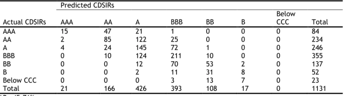
The distribution of firms by rating categories for CDSIRs and EQIRs are reported in Table 2-2 and Table 2-3 respectively. Based on these tables, there is no significant difference in the distribution of firms across the rating categories and most firms are assigned A and BBB ratings.
Chapter 2 2.3 Data and summary statistics Table 2-2 CDSIRs of firms by year
AAA AA A BBB BB B Below CCC Number of Observations 2002 4 35 46 32 20 1 0 138 2003 10 44 68 65 32 7 0 226 2004 11 41 60 70 35 10 0 227 2005 9 34 57 71 29 10 1 211 2006 9 24 52 63 26 4 1 179 2007 14 45 54 63 28 13 6 223 2008 12 19 13 33 13 3 1 94 Number of Observations 69 242 350 397 183 48 9 1298
Note: This table presents the distribution of firms by rating category for CDSIRs by year.
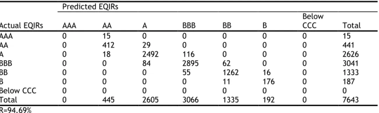
Table 2-3 EQIRs of firms by year
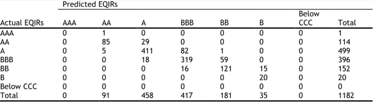
AAA AA A BBB BB B Below CCC Number of Observations 2002 1 13 55 103 76 16 0 264 2003 2 19 91 106 43 5 0 266 2004 1 20 100 99 42 6 0 268 2005 0 10 70 87 38 4 0 209 2006 0 11 80 74 29 4 0 198 2007 1 19 91 80 41 8 0 240 2008 0 5 29 37 23 1 0 95 Number of Observations 5 97 516 586 292 44 0 1540
Note: This table presents the distribution of firms by rating category for EQIRs by year.
At the next stage, summary statistics for our explanatory variables are documented in Table 2-4 and Table 2-5. To capture any differences across ratings categories, the sample is separated into investment grades and non-investment grades and then statistics are presented. We report p-values for the tests of equality of means across the above-mentioned groups in the last columns of the tables. It can be observed that firms in the investment grade group experience better financial conditions, as measured by the accounting ratios from the balance sheet. This is consistent with our expectations. The significant differences between the two groups can be confirmed from tests, which suggest that there exists a link between better financial health and an improved rating. In other words, the cross-sectional variation can be observed in market implied ratings.
Moving to the market indicators, it can be confirmed that improved market conditions are associated with the rating changes, which also suggests a relation between the market climate and the ratings.
Table 2-4 Descriptive statistics-CDSIRs
Variable Mean
Standard
Deviation Minimum Maximum p-value
(1) (2) (3) (4) (5) DETA Investment grade 9.6388 1.0132 7.2272 12.2084 0.0000 Non-investment grade 8.9536 0.9959 6.2539 12.2087 AE Investment grade 3.2256 3.6336 1.3324 73.7340 0.0000 Non-investment grade 5.0224 8.8729 1.3283 123.5602 LDA Investment grade 20.2416 11.2733 0.0000 79.3983 0.0000 Non-investment grade 30.1868 19.4641 0.0000 110.4453 SDA Investment grade 3.5941 3.9838 0.0000 23.5410 0.0000 Non-investment grade 3.2961 4.1573 0.0000 23.4635 TDA Investment grade 24.3546 11.9238 1.3017 87.0595 0.0000 Non-investment grade 37.4629 20.8746 0.6518 126.8760 TDEBITDA Investment grade 2.3395 1.2107 0.3200 19.6400 0.0000 Non-investment grade 4.1208 2.8918 0.3200 23.0700 EBITINT Investment grade 13.3805 19.0270 0.1541 209.3023 0.0000 Non-investment grade 7.2685 15.2730 0.1248 210.4054 EBITDAINT Investment grade 16.0444 21.9950 0.6500 235.4000 0.0000 Non-investment grade 9.0872 14.5213 0.3100 196.7000 CFOA Investment grade 6.9186 6.2625 -41.0623 38.4372 0.0000 Non-investment grade 7.1077 7.2097 -13.4106 65.9955 CASHEQA Investment grade 8.6116 9.6531 0.0238 71.8277 0.0000 Non-investment grade 6.5258 8.1009 0.0030 64.0272 OM Investment grade 13.9496 9.7304 -13.5155 53.0189 0.0000 Non-investment grade 10.3893 9.9617 -20.2276 52.6046 ROC Investment grade 3.7919 5.3598 -34.1330 35.7771 0.0000 Non-investment grade 2.1389 7.0866 -36.3880 34.5209 ROE