Supervised and unsupervised weight and delay adaptation learning in temporal coding spiking neural networks

CARDIFF

C

RDY|§>

Su p ervised and u n su p ervised

w eight and delay a d a p ta tio n learning

in tem p o ra l cod in g

spiking neural netw orks

A thesis submitted to the Cardiff University,

for the degree of

D octor o f P h ilosop h y

by

E ugene Y ougarajah A ndrew Charles

Manufacturing Engineering Centre

Cardiff University

UMI Number: U584933

All rights reserved

INFORMATION TO ALL USERS

The quality of this reproduction is dependent upon the quality of the copy submitted. In the unlikely event that the author did not send a complete manuscript and there are missing pages, these will be noted. Also, if material had to be removed,

a note will indicate the deletion.

Dissertation Publishing

UMI U584933

Published by ProQuest LLC 2013. Copyright in the Dissertation held by the Author. Microform Edition © ProQuest LLC.

All rights reserved. This work is protected against unauthorized copying under Title 17, United States Code.

ProQuest LLC

789 East Eisenhower Parkway P.O. Box 1346

A bstract

Artificial neural networks are learning paradigms which mimic the biological neu­ ral system. The temporal coding Spiking Neural Network, a relatively new artifi­ cial neural network paradigm, is considered to be computationally more powerful than the conventional neural network. Research on the network of spiking neurons is an emerging field and has potential for wider investigation. This research ex­ plores alternative learning models with temporal coding spiking neural networks for clustering and classification tasks.

Neurons are known to be operating in two modes namely, as integrators and coincidence detectors. Previous temporal coding spiking neural networks, realis­ ing spiking neurons as integrators, were utilised for analytical studies. Temporal coding spiking neural networks applied successfully for clustering and classifica­ tion tasks realised spiking neurons as coincidence detectors and encoded input in­ formation in the connection delays through a weight adaptation technique. These learning models select suitably delayed connections by enhancing the weights of those connections while weakening the others. This research investigates the learning in temporal coding spiking neural networks with spiking neurons as integrators and coincidence detectors. Focus is given to both supervised and unsupervised learning through weight as well as through delay adaptation.

Three novel models for learning in temporal coding spiking neural networks are presented in this research. The first spiking neural network model, Self- Organising Weight Adaptation Spiking Neural Network (SOWA_SNN) realises the spiking neuron as integrator. This model adapts and encodes input informa­ tion in its connection weights. The second learning model, Self-Organising Delay Adaptation Spiking Neural Network (SODA_SNN) and the third model, Super­ vised Delay Adaptation Spiking Neural Network (SDA_SNN) realise the spiking

iii

neuron as coincidence detector. These two models adapt the connection delays in order to detect temporal patterns through coincidence detection. The first two models were developed for clustering applications and the third for classifica­ tion tasks. All three models employ Hebbian-based learning rules to update the network connection parameters by utilising the difference between the input and output spike times.

The proposed temporal coding spiking neural network models were imple­ mented as discrete models in software and their characteristics and capabilities were analysed through simulations on three bench mark data sets and a high dimensional data set. All three models were able to cluster or classify the anal­ ysed data sets efficiently with a high degree of accuracy. The performance of the proposed models, was found to be better than the existing spiking neural network models as well as conventional neural networks. The proposed learning paradigms could be applied to a wide range of applications including manufacturing, business and biomedical domains.

to the loving memory of my father

A cknow ledgem ents

I would like to express my deep and sincere gratitude to my supervisor, Dr. M. S. Packianather. His wide knowledge and logical way of thinking have been of great value for me. His understanding, encouraging and personal guidance have provided a good basis for the present thesis. I am deeply grateful to my supervisor, Professor D. T. Pham, for his detailed and constructive comments, and for his important support throughout this work. My sincere thanks also goes to Professor S. S. Dimov for his suggestions and comments throughout this work.

I wish to express my warm and sincere thanks to Dr. S. Mahesan for his tireless and generous effort which gave me the opportunity to do this research. My sincere thanks also belong to Dr. S. Kanaganathan. I wish to express my thanks to all the staff, colleagues and friends of University of Jaffna, Sri Lanka.

I would like to thank all my colleagues specially for the Data mining group mem­ bers, for their guidance and company. My sincere thanks also to all the staff of the Manufacturing Engineering Centre. I wish to express my special thanks to all my friends in Cardiff, London and elsewhere.

My special gratitude is due to my mother, aunty, brother and my sister for their love and encouragement.

D eclaration

This work has not previously been accepted in substance for any degree and is not concurrently submitted in candidature for any degree.

Signed . . (Eugene Yougarajah Andrew Charles - Candidate) D ate.

Statem ent 1

This thesis is being submitted in partial fulfilment of the requirements for the degree of PhD.

Signed . YqW . (Eugene Yougarajah Andrew Charles - Candidate)

Statem ent 2

This thesis is the result of my own independent work/investigation, except where otherwise stated. Other sources are acknowledged by explicit references.

Date . A J : P.1: A ™ * .

Statem ent 3

I hereby give consent for my thesis, if accepted, to be available for photocopy­ ing and for inter-library loan, and for title and summary to be made available to outside organisations.

Date . : °.cf. A?Pf>

(Eugene Yougarajah Andrew Charles - Candidate)

Signed (Eugene Yougarajah Andrew Charles - Candidate) Date . A 7^'. Pf^: P~P? ^

Contents

List o f Figures xiii

List o f Tables xvi

List o f Sym bols xviii

1 Introduction 1

1.1 Preliminaries ... 2

1.2 Research o b jectiv es... 5

1.3 Structure of the t h e s i s ... 6

2 T he basics o f Spiking Neural Networks 8 2.1 Artificial Neural N e tw o rk s... 9

2.1.1 Structure of the artificial neural n e tw o rk ... 9

2.1.2 The artificial n e u r o n ... 10

C O N T E N T S_____________________________________________________ viii 2.2 Biological background ... 16 2.2.1 The n e u r o n ... 17 2.2.2 The sy n ap se... 18 2.2.3 Electrical properties of n e u r o n s ... 20 2.2.4 Neuronal f i r i n g ... 22 2.3 Neuronal coding... 23 2.3.1 Rate c o d in g ... 24

2.3.2 Temporal coding (Spike c o d in g )... 24

2.3.3 Population coding... 26

2.3.4 On the coding of neural inform ation... 26

2.4 Neuron models ... 27

2.4.1 Conductance-based neuron models ... 28

2.4.2 Spiking neuron m o d e ls ... 30

2.4.3 Spike response m o d e l... 30

2.5 The spiking neural network ... 32

2.5.1 Definition of the spiking neural network ... 32

2.5.2 Computing with spiking neural network ... 35

2.5.2.1 Realising a p e rc e p tro n ... 35

2.5.2.2 Computing a weighted s u m ... 36

2.5.2.3 Coincidence d e te c t i o n ... 37

2.5.3 Spiking neural network sim ulators... 40

2.5.4 Discrete spiking neural network m o d e l ... 41

2.5.5 Learning in spiking neural netw orks... 43

2.6 Research a p p lic a tio n ... 47

2.6.1 Clustering and classification... 48

2.6.2 Description of the data s e t s ... 49

C O N T E N T S______________________________________________________ ix 3 Self-Organising W eight A daptation

Spiking Neural Network (SOW A_SNN) 54

3.1 In tro d u ctio n ... 54

3.2 Kohonen’s self-organising m a p ... 55

3.3 Research on unsupervised SNN models and biological neural net­ works 59 3.3.1 Weight-based l e a r n in g ... 60

3.3.2 Delay based le a r n in g ... 61

3.3.3 Research on biological neural n e tw o rk s ... 67

3.3.3.1 Learning in biological neural n e tw o rk s ... 67

3.3.3.2 Spike-time-based le a r n in g ... 69

3.3.3.3 Stabilising the Hebbian learning... 70

3.4 Proposed self-organising weight adaptation SNN for clustering . . 74

3.4.1 Network a rc h ite c tu re ... 74

3.4.2 Spike time based learning ... 75

3.4.3 Self-organisation ... 75

3.4.4 Stabilising the weight a d a p ta tio n ... 77

3.4.5 Learning r u l e ... 78

3.4.6 Learning s tr a te g y ... 78

3.4.7 Interpreting the output and cluster identification ... 80

3.5 Implementation d e ta ils ... 81

3.5.1 Initialising the connection weights and d e l a y s ... 83

3.5.2 Setting the threshold v a lu e ... 84

3.5.3 Setting the parameters of the learning r u l e ... 84

3.6 Simulation results and d is c u s s io n ... 85

3.6.1 Clustering c a p a b ility ... 85

3.6.2 S ta b ility ... 96

C O N T E N T S x 4 Self-Organising D elay A daptation

Spiking Neural Network (SO DA_SNN) 103

4.1 In tro d u ctio n ...103

4.2 Neuronal delays and coincidence d e te c tio n ... 104

4.2.1 Neural systems and D elays... 104

4.2.2 Neuron as a coincidence d e t e c t o r ...105

4.2.3 The operating mode of a n e u ro n ... 106

4.2.4 Pattern detection with coincidence detecting spiking neuron 107 4.2.5 Delay adaptation le a r n in g ... 107

4.3 Research on delay adaptation learning ... 110

4.3.1 Delay-based modelling s tu d ie s ... 110

4.3.2 Learning models for conventional networks with delays . . I l l 4.3.3 Delay adaptation learning in S N N s ...112

4.4 Proposed self-organising delay adaptation SNN for clustering . . . 113

4.4.1 Network a rc h ite c tu re ...113

4.4.2 Integration and coincidence detection with a spiking neuron 114 4.4.3 Spike time-based delay adaptation learning...115

4.4.4 Self-organisation ...116

4.4.5 Stabilising the delay a d a p ta tio n ... 118

4.4.6 Learning r u l e ... 119

4.4.7 Interpreting the output and cluster identification ... 120

4.5 Implementation d e ta ils ...120

4.5.1 Initialising the connection weights and delays ... 121

4.5.2 Setting the threshold v a lu e ... 122

4.5.3 Setting the parameters of the learning r u l e ... 123

4.6 Simulation results and d is c u s s io n ...123

4.6.1 Clustering c a p a b ility ...124

C O N T E N T S______________________________________________________ xi

4.6.3 Degree of coincidence... 132

4.6.4 S ta b ility ...141

4.7 Conclusion... 151

5 Supervised D elay A daptation Spiking Neural Network (SD A_SNN) 153 5.1 In troduction... 153

5.2 Supervised learning in artificial neural n e tw o rk s ...154

5.2.1 Supervised learning in conventional neural networks . . . . 155

5.2.2 Supervised learning in spiking neural netw orks...158

5.2.2.1 Error gradient based learning m o d e ls... 159

5.2.2.2 Hebbian rule based learning m odels... 162

5.3 Proposed supervised delay adaptation SNN for classification . . . 164

5.3.1 Network a rc h ite c tu re ... 164

5.3.2 The learning r u l e ... 165

5.3.3 Delay change e s tim a tio n ... 167

5.3.4 Controlling the l e a r n in g ... 168

5.3.5 Interpreting the results and classifying the input data . . . 169

5.3.6 The training p r o c e s s ... 170

5.4 Implementation d e ta ils ... 171

5.5 Simulation results and d is c u s s io n ...171

5.5.1 Classification capability ... 172

5.5.2 Network a c t i v i t y ...175

5.5.3 Degree of coincidence... 175

5.5.4 S ta b ility ...178

5.6 Conclusion... 184

6 C onclusion and future work 185 6.1 C o n trib u tio n s... 185

C O N T E N T S_____________________________________________________ xii

6.2 Conclusion... 188

6.3 Future w o r k ... 190

B ibliography 192 A ppendices 202 A Program source code 203 A.l Class definitions... 203

A. 1.1 Definition of class V ector... 203

A. 1.2 Definition of class m a trix...204

A. 1.3 Definition of class spikeNN ...205

A.2 Source code for implementing the unsupervised m o d e ls ... 207

A.2.1 Source code for implementing the S N N ...207

A.2.2 Source code for implementing SOWA_SNN... 210

A.2.3 Source code for implementing SO D A _SN N ... 212

A.2.4 Section of class spikeNN for testing the data sets ... 215

A.2.5 Source code for clustering Wine data set with SOWAJSNN 217 A.2.6 Source code for clustering Iris data set with SODAJ3NN . 221 A.3 Source code for implementing S D A J3 N N ...224

List o f Figures

2.1 General structure of an artificial neural n e tw o rk ... 11

2.2 Schematic diagram of an artificial n e u ro n ... 12

2.3 Common activation f u n c tio n s ... 13

2.4 Schematic diagram of a neuron ... 19

2.5 S y n a p s e ... 21

2.6 An equivalent circuit for the Hodgkin-Huxley m o d e l... 29

2.7 Spike response f u n c tio n s ... 33

2.8 Coincidence detection by a spiking n e u r o n ... 39

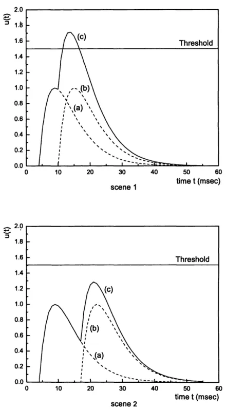
2.9 Control chart p a t t e r n s ... 53

3.1 Kohonen’s self-organising n etw o rk ... 57

3.2 Gerstner et al.s’ learning rule ... 64

3.3 Natschlager and Rufs’ network m o d e l... 65

3.4 Natschlager and Rufs’ learning rule for unsupervised learning . . . 66

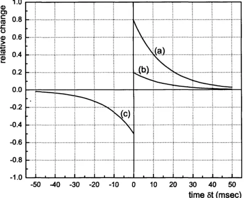
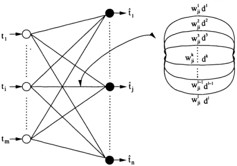
3.5 Song et al.s’ learning rule for unsupervised le a r n in g ... 71

3.6 van Rossum et al.s’ rule for synaptic m o d ificatio n ... 73

3.7 Learning rule for the SOWA_SNN... 76

3.8 Clusters formed within Iris data set using SO W A _SN N ... 88

3.9 Clusters formed within the Cancer data set using SOWA_SNN . . 89

3.10 Clusters formed within Wine data set using SO W A_SNN... 90 3.11 Clusters formed within Control chart data set using SOWA_SNN . 91

LIST OF FIG URES______________________________________________ xiv

3.12 Distribution of the connection weights of the SOWA_SNN trained

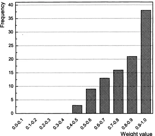
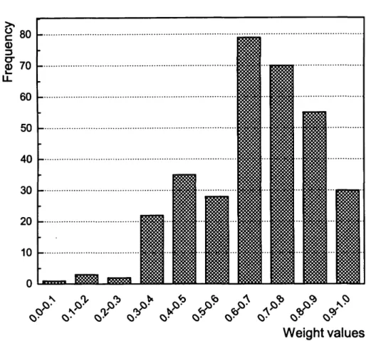
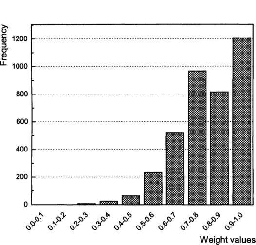
on Iris d ata... 98

3.13 Distribution of the connection weights of the SOWA_SNN trained on Cancer data... 99

3.14 Distribution of the connection weights of the SOWA_SNN trained on Wine data... 100

3.15 Distribution of the connection weights of the SOWA_SNN trained on Control chart d ata... 101

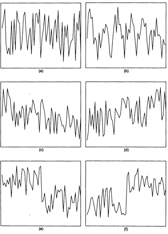
4.1 Pattern detection by spiking neural n e tw o r k ... 108

4.2 Learning rule for delay ad ap tatio n ... 117

4.3 Activity of the SODAJ3NN trained on Iris d a t a ... 133

4.4 Activity of the SODA_SNN trained on Cancer d a t a ...134

4.5 Activity of the SODA_SNN trained on Wine d a t a ...135

4.6 Activity of the SODA_SNN trained on Control chart d a t a 136 4.7 Clusters formed within the Iris data using SODA_SNN with dy­ namic and fixed t h r e s h o ld ...137

4.8 Clusters formed within the Cancer data using SODA_SNN with dynamic and fixed th re s h o ld ...138

4.9 Clusters formed within the Wine data using SODA_SNN with dy­ namic and fixed t h r e s h o ld ...139

4.10 Clusters formed within the Control chart data using SODA_SNN with dynamic and fixed th re s h o ld ... 140

4.11 Degree of coincidence achieved in the SODA_SNN trained on Iris d a t a ...142

4.12 Degree of coincidence achieved in the SODA-SNN trained on Can­ cer d a t a ...143

4.13 Degree of coincidence achieved in the SODA_SNN trained on Wine d a t a ...144

4.14 Degree of coincidence achieved in the SODA_SNN trained on Con­ trol chart d a ta ... 145

4.15 Delay distribution of the SODA_SNN trained on Iris d a t a ... 147

LIST OF FIG U R ES xv

4.17 Delay distribution of the SODA.SNN trained on Wine data . . . . 149 4.18 Delay distribution of the SODA_SNN trained on Control chart data 150

5.1 Schematic diagram of supervised learning...156 5.2 Population coding with overlapping Gaussian receptive fields . . . 161 5.3 Structure of the supervised delay adaptation S N N ... 166 5.4 Distribution of the delays in the SDAJ3NN trained on Iris data . . 180 5.5 Distribution of the delays in the SDA_SNN trained on Cancer data 181 5.6 Distribution of the delays in the SDAJ3NN trained on Wine data 182 5.7 Distribution of the delays in the SDA_SNN trained on Control

List o f Tables

2.1 Description of the data s e t s ... 51

3.1 Number of samples used for training and te s tin g ... 87

3.2 Average clustering accuracy obtained for the SOWA_SNN... 93

3.3 Network parameter values for the SOWA_SNN... 93

3.4 Clustering accuracy obtained for different size of SOWA_SNNs . . 94

3.5 Average clustering accuracy obtained on Control chart data for different size of SOWA_SNNs ... 94

3.6 Average clustering accuracy obtained for Kohonen’s SO M ... 97

3.7 Average highest clustering accuracy obtained for Kohonen’s SOM 97 4.1 Average clustering accuracy obtained for the SO D A .SN N ... 126

4.2 Network parameter values for the SODA_SNN... 126

4.3 Clustering accuracy obtained for different size of SODA_SNNs . . 127

4.4 Average clustering accuracy obtained on Control chart data for different size of SODA_SNNs...127

4.5 Average clustering accuracy obtained for Kohonen’s S O M ...130

4.6 Average highest clustering accuracy obtained for Kohonen’s SOM 130 4.7 Details of the SODA_SNNs for the analysis of network activity . . 131

5.1 Average classification accuracy obtained for the SDA_SNN . . . . 173

5.2 Network parameter values for the SD A J3N N ... 173

5.3 Classification accuracy for Bohte et al.s’ m o d el... 176

5.4 Average classification accuracy obtained for M L P ... 176

LIST OF TABLES______________________________________________ xvii

5.5 Average highest classification accuracy obtained for M L P ...177 5.6 Activity of the SDA.SNN ... 177 5.7 Degree of coincidence achieved by the SDAJ3NN... 179

List o f Sym bols

Sdji The amount of change for delay to the connection from neuron i to j e The spike response function

V Learning rate

To Set of neurons pre-synaptic to neuron j

N Set of all natural numbers

R + Set of all positive real numbers (excluding zero) R Set of all real numbers

Si Set of all previous firing times of neuron i

<t> Activation function

T Time constant for the spike response function

Tstdp Synaptic time constant for potentiation and depression of the learning

rule

0 Refractory function of neuron j

bj Bias value for neuron j

dji Delay value of the connection from neuron i to j dt Time step between the adjacent states of simulation

dwji Change in weight for the connection from neuron i to j E Set of synapses

N A network of neurons

t time

Unputjmndow Input time window

twindow Activation time window

U j { t ) Potential or state variable of neuron j at time t

List o f Sym bols xix

V Set of neurons

Vj Linearly combined output of the weighted input signals to neuron j

Wji Strength or weight of the connection from neuron i to j Xi Input value to neuron i

yj Output of neuron j ||w|| Euclidean norm of w

Chapter 1

Introduction

Artificial neural networks (ANNs) are one of the most powerful and flexible com­ puting paradigms and a well studied area in artificial intelligence. The important property of an ANN is its ability to learn from the environment and to retain in­ formation. The development of ANN was inspired by the principles of biological neural networks which process information in an entirely different way from con­ ventional methods. The modern era of ANNs was initiated with the pioneering work of McCulloch and Pitts [McCulloch and Pitts, 1943]. From then on, the research on ANNs grew in different directions and led to the creation of various artificial neurons, network architectures and learning algorithms. As a result, ANNs have been applied successfully for solving diverse problems in numerous domains [Haykin, 1999].

In recent years, temporal coding Spiking Neural Networks (SNN), networks of more biologically realistic artificial neurons, are receiving wider attention. Re­ sults from past research show that the learning in spiking neural networks can achieve the accuracy of conventional training algorithms with potential room for improvement [Bohte et al., 2002a]. This research explores alternative learning ap­ proaches for temporal coding SNNs for clustering and classification tasks. This chapter presents the preliminaries regarding the SNNs and defines the objectives

1.1 Prelim inaries 2

of this research. The structure of this research is also outlined here.

1.1

Prelim inaries

The human brain, the most interesting and important organ in the world, has revealed only a few of its secrets to humankind. Even though the exploration of the brain began 2500 years ago when Greek philosophers conceived the idea that the human beings have a mind and a soul, researchers managed to shed some light on the true nature of the brain only within the past hundred years. The study on biological neural systems is developing more rapidly and attracts people from various disciplines. The findings from these studies not only provide a better understanding of neural systems but also shape the research on artifi­ cial intelligence. Although the creation and development of ANNs were inspired by biological neural systems, ANNs are considered to be limited due to their simplistic structure and behaviour [Zador, 2000; Maass, 1997a].

The brain is composed of billions of simple computing elements called neu­ rons which are connected in parallel with trillions of interconnections or synapses

[Haykin, 1999]. Artificial neural networks axe also structured similarly, with in­ terconnected computational units. The interconnections between the neurons in a conventional artificial neural network are considered as passive entities. These synapses are regarded as simple linear entities whose essential role is in learn­ ing. But it is claimed by the neuro biologists that the biological synapses are not merely passive entities whose outputs are a linear function of their inputs. Instead, it has been recognised for a long time that the synapses are dynamic elements with complex non-linear behaviour [Zador, 2000].

Computation and communication within the biological networks are based on action potentials or spikes. The spikes are electrical pulses with a potential

1.1 Prelim inaries 3

of around 100 mV and last for one to two msec. The way the information is coded with these spikes is an ongoing debate. In general it is accepted that the coding could be either based on the rate of spikes or on the firing time of each spike. Artificial neural networks were developed based on the idea that the biological neurons communicate via the firing rate of spikes [Bohte, 2003]. Generally, the analogue values responsible for computation and communication in the conventional artificial neural networks are interpreted as the firing rates of biological neurons [Maass, 1997a]. In recent years, however, the notion of rate of spikes is claimed to be inadequate for the operation of fast neuronal events. On the other hand, spike time-based coding or temporal coding are found to be competent and widely accepted [Gerstner and Kistler, 2002].

The disputes over the structure and functionality of conventional artificial neural networks resulted in increased interest in temporally coding spiking neu­ ral networks. These networks incorporate the non-linear nature of the synapses and are capable of dealing with spike-time based coding. It has been proved that the networks of spiking neurons can simulate arbitrary feed-forward sig­ moidal neural networks and thus approximate any continuous function [Maass, 1997a]. It was also proved that neurons that convey information by the timing of individual spikes are computationally more powerful than the classical neurons with sigmoidal activation function [Maass, 1997c]. Another feature of the spiking neurons is that even with a seemingly increased structural complexity they are relatively easier to implement in large neural networks [Bohte et al., 2002a]. Sin­ gle spike-time based computing has also been suggested as a new paradigm for VLSI neural network implementation [Maass, 1996]. It was also observed that there is considerable opportunity for further research on SNN, with potential improvement in various directions [Maass, 2001b].

1.1 Prelim inaries 4

value and a delay mechanism which postpones the arrival of an input spike at the other end of the connection. It is understood that biological neurons operate in two modes, as integrators and as coincidence detectors [Konig et al., 1996]. Generally, artificial neurons are known to be integrators, but due to the connec­ tion delays, the spiking neurons exhibit the coincidence detection functionality

[Maass, 2001a]. In this mode, a spiking neuron is activated only when it receives coinciding inputs. The identification of these two modes of operations of a spiking neuron is supported by several studies on biological neurons [Konig et al., 1996].

Temporal coding SNNs can be applied to the same types of tasks as con­ ventional ANNs. Recently a number of researchers have carried out significant research on learning with spiking neural networks. In general, the learning models adapt the connection weights and attem pt to encode the input information in the connection weights and delays. A significant number of learning models proposed in the past for spiking neural networks are based on the Hebbian rule [Natschlager and Ruf, 1998; Bohte et al., 2002b]. This is a preferred approach due to the nature of the spiking neurons’ functionality and the spike-time based information coding strategy. Error gradient descent approaches have also been proposed and applied successfully [Bohte et al., 2002a]. A significant amount of research has targeted the pattern recognition, clustering and classification tasks as the main application for their proposed models [Ruf and Schmitt, 1997; Natschlager and Ruf, 1998; Ruf and Schmitt, 1998; Bohte et al., 2002b]. In addition, several examples can be found in the literature where the spiking neural networks have been applied to various other learning tasks such as function approximation [Iannella and Back, 2001], associative memory and speech recognition [Bohte and Kok, 2005].

1.2 Research objectives 5

1.2

R esearch objectives

The main objective of this research is to investigate the possible supervised and unsupervised learning strategies for temporal coding spiking neural networks and to develop alternative learning models. The focus of this research is on learning models which adapt network connection weights as well as delays for clustering and classification tasks. More details are given in section 2.7.

Most of the existing learning models for spiking neural networks are based on the learning models for conventional neural networks. But it is here claimed that for spiking neural networks, the learning strategies have to be developed distinctively in order to exploit the full potential of spiking neurons. However, this is relatively difficult to achieve without the knowledge of learning strategies of biological neural networks. Fortunately, there are plenty of research findings on learning in biological networks available which are yet to be incorporated in the development of artificial neural networks. Hence another objective of this research is to combine the knowledge gained from the valuable research on biological neural networks and the knowledge available from the existing ANN learning models in order to develop novel models for learning in spiking neural networks.

SNNs can be implemented in software as well as hardware. In this research, developing a suitable software platform is considered as an objective in which the spiking neural network learning models can be realised and analysed.

The research on learning in spiking neural networks is at a relatively early stage. The analysis on networks of spiking neurons is important for creating better network models and learning strategies. Providing analytical results on various aspects of the network models and learning strategies is also considered as an objective of this research.

1.3 Structure of the thesis 6

1.3

Structure o f th e th esis

This study consists of six chapters and two appendices. Chapter 2 summarises the basics of temporal coding spiking neural network. This chapter starts with a description of artificial neural networks and methods through which they learn. A brief outline of the biological neural network is also included. Aspects of neuronal coding and various neuron models are discussed. The temporal coding spiking neural network is introduced and topics regarding computing with SNNs and re­ alising the network are explained. Previous research on learning in spiking neural networks is summarised. Further, a description of clustering and classification, the main application of this study, is given along with the details of the data sets utilised. Finally, this chapter concludes with an outline of this research.

This research focuses on learning in spiking neural networks through adapting the connection weights as well as delays by supervised and unsupervised learning methods. Chapter 3 focuses on learning through weight adaptation in an un­ supervised manner. This chapter briefly describes the Kohonen’s self-organising map (SOM), which is a popular unsupervised learning model for artificial neural networks. Previous research on SNNs regarding the unsupervised and Hebbian- based learning is summarised along with the key findings on learning in biolog­ ical neural networks. The Self-Organising Weight Adaptation Spiking Neural Network (SOWA_SNN) is introduced and the details regarding its implementa­ tion are given. Finally, the results of the analytical studies conducted on the proposed model are summarised and discussed.

Most of the previous research on learning with spiking neural networks adapts the connection weights. Chapter 4 proposes an unsupervised learning model for SNNs, in which the connection delays are adapted. Here the spiking neurons are realised as coincidence detectors, and delays and coincidence detection are

1.3 Structure of the thesis 7

explained in this chapter. Previous work on delay adaptation learning is sum­ marised. The details about the proposed Self-Organising Delay Adaptation Spik­ ing Neural Network (SODAJSNN) are presented along with the implementation details. Finally, the description of the analytical studies performed on the pro­ posed model is explained and the results obtained are summarised and discussed.

Chapter 5 deals with learning in spiking neural networks in a supervised man­ ner, where the spiking neurons are realised as coincidence detectors, as in chapter 4. This chapter briefly describes supervised learning models in artificial neural networks and summarises previous supervised learning models for spiking neu­ ral networks. The novel Supervised Delay Adaptation Spiking Neural Network

(SDA_SNN) is introduced and the details regarding its implementation are given. The details of the analytical studies conducted are presented and the chapter concludes with the summary of the results obtained along with the discussion.

Each chapter ends with a brief conclusion covering the topics discussed in that chapter. Chapter 6 gives the conclusions drawn form this whole research and presents some suggestions for future work.

Appendix A presents the source code of the software developed to implement the proposed learning models.

Appendix B provides the data sets used for training and testing the proposed models.

Chapter 2

The basics of Spiking Neural

Networks

Spiking neurons are claimed to be the third generation of artificial neurons with

McCulloch-Pitts [Haykin, 1999] neurons as the first generation and neurons with

continuous activation functions (sigmoidal neurons) as the second generation [Maass, 1997b]. This chapter lays the foundation for this study by introduc­ ing the basics of SNNs. In order to get a better understanding of SNNs, topics regarding the neural network models of both artificial and biological systems and other related themes are explained in this chapter.

This chapter is structured as follows: section 2.1 introduces the concept of artificial neural networks and related topics; section 2 . 2 explains the biological neural system and how it forms the basis for artificial neural networks. Neuronal coding, i.e., the way in which the information is coded in biological neural systems is summarised in section 2.3, and neuron models are described in section 2.4. The spiking neural network is defined in section 2.5. This section includes details of computing with SNNs and the realisation of the network. The previous research on learning in SNNs is also summarised in this section. Section 2.6 introduces the application area of this research, namely, clustering and classification. The details of the data sets used for analytical studies are also described in this section.

2.1 Artificial Neural Networks 9

Finally, section 2.7 defines the outline of this research.

2.1

A rtificial N eural N etw orks

An artificial neural network (ANN) is an information processing paradigm made up of simple processing units analogous to a massively parallel distributed proces­ sor. The simple computational units are called neurons after biological neurons, which were the inspiration for this method of information processing [Haykin, 1999]. This relatively new computational tool has found its way into solving many complex problems successfully and efficiently. The important characteris­ tics of ANNs are non-linearity, high parallelism, fault and noise tolerance, learning and generalisation capabilities [Jain et al., 1996].

2.1.1

Stru ctu re o f th e artificial neural netw ork

The structure or topology of an ANN defines the way the neurons are placed in the network and the way in which they are connected to one another. The structure of the network plays an important role in information processing since it is closely linked to the learning algorithm used to train the network. Generally, in an ANN, neurons are placed in layers. A network can have more than one layer of neurons in addition to the input layer. The input layer is simply a set of non-processing nodes from where the inputs are fed to the network. Neurons in each layer are connected to neurons in other layers through a set of links. A typical structure of an ANN is shown in Figure 2.1. Although it is not shown in this figure, neurons within a layer can also be connected one to another through lateral connections. The output from a neuron is passed to the other neurons through these links. Depending on the direction of flow of information, the network is referred to as a feed-forward network or a recurrent network. In the former, the flow is in

2.1 Artificial Neural Networks 10

the forward direction only and in the latter the flow can be both in forward and as well as backward direction. Each link or connection is characterised by a weight value, which is known as the connection strength. These connections are the pathways for the information within the network [Haykin, 1999]. The processing of information is performed by a neuron which is described in the next sub-section.

2.1.2

T h e artificial neuron

A neuron is the fundamental processing unit of an ANN as in a biological neural network. Figure 2.2 shows a formal base model of a neuron. The output of a neuron is the linear weighted sum of its inputs subjected to an activation function. Equations 2.1 and 2.2 define the output of an artificial neuron [Pham and Liu,

where Xi, i = 1 ..n are the input values and bj is the bias value. Wji, i = l..n are the connection weights for neuron j from neuron i. Here n is the number of input neurons. Vj is the intermediate output which is passed to the activation function

(f) to produce the final output yj.

There are several forms of activation functions from which a suitable one can be selected according to the target application. Common activation functions are

threshold function, piecewise linear function and sigmoidal function, which are

shown in figure 2.3 [Haykin, 1999]. The important feature of the artificial neural networks made up of these simple processing units is their ability to learn and retain information from their environment. Learning in ANNs is discussed in the next sub-section.

1999].

n

(2.1)

2.1 Artificial Neural Networks 11 bias input Input jc( Output layer Hidden layer y i Output Input layer

2.1 Artificial Neural Networks 12 input bias b output jn—1 n - i Neuron j

Figure 2 .2 . Schematic diagram of an artificial neuron. Redrawn from [Pham and Liu, 1999].

2.1 Artificial Neural Networks 13 .0 0 M 0.75 0.5 0.25 0.0 0.0 0.5 - 1.5 - 1.0 - 0.5 1.0 1.5 v

(a) Threshold function

1.0 (j) (v) 0.75 0.5 0.25 0.0 - 1.5 - 1.0 - 0.5 0.0 0.5 1.0 1.5 v

(b) Piecewise linear function

<j) (v) 0.75 0.5 0.25 0.0 -12 •8 - 4 0 4 8 12 v (c) Sigmoidal function

2.1 Artificial Neural Networks 14

2.1.3

Learning in artificial neural netw orks

The most significant property of the neural system is its ability to learn from its environment and so improve its performance. In the context of learning in arti­ ficial neural networks, learning can be defined as follows: “Learning is a process by which the free parameters of a neural network are adapted through a process of

simulation by the environment in which the network is embedded” [Mendel and

McLaren, 1970]. Likewise, an ANN also posses this important feature. With the aid of a learning procedure, the ANNs can extract and store information from the data made available to the network. The extracted information is stored in the network through the connection weights, and can be retrieved for future use. The learning in the ANNs can either be with a teacher (supervised learning) or without a teacher (unsupervised learning). In supervised learning the network is presented with a set of input-output examples. Based on the output for a given example, the teacher will specify a desired output which the network is expected to produce. The difference between the actual output and the desired output is called an error signal. The objective of the training procedure is to modify the network parameters in such a way that the network produces an out­ put which is as close as possible to the desired output, thus reducing the error. The modification is based on both the input signal and the error signal [Haykin, 1999].

For unsupervised learning, the examples presented are not labelled and the learning is performed without any external supervision. There are two modes in this form of learning, namely, self-organising learning and reinforcement learn­ ing. In self-organising learning the network undergoes change of its parameters according to its learning rules without any supervision. The modifications to the network parameters are performed in such a way that the network automatically

2.1 Artificial Neural Networks 15

discovers for itself any possibly existing patterns, regularities, separating proper­ ties etc. in the presented data [Zurada, 1999]. Even though the reinforcement learning comes under the category of unsupervised learning, it can be considered as a special case of supervised learning because of the use of a critic to control the learning. Unlike in the case of supervised learning, here the critic evaluates the quality of the output produced by the network for a given input signal. Modifi­ cation to the network parameters are based on this criticism and the input signal [Pham and Liu, 1999].

Supervised and unsupervised learning are known as learning paradigms. In both models the actual modifications to the network parameters are performed through learning-rules. There are five basic learning rules mentioned in the litera­ ture. They are error-correction learning, memory-based learning, Hebbian learn­

ing, competitive learning and Boltzman learning [Haykin, 1999]. Error-correction

learning, as the name suggests, tries to correct an error estimation. For a par­ ticular training sample, the difference between the actual output of the network and a desired output is considered as the error. The learning is performed in such a way that the network is enabled to give an output as close as possible to the desired output, thus reducing the error.

Memory-based learning functions by storing all the past experience or training samples (xi? di) explicitly in a large memory. Here (x*, di) are correctly classified input-output samples. Classification of an unseen sample is done by retrieving and analysing a training sample from the stored memory which falls within the logical neighbourhood of this new sample [Haykin, 1999].

The Hebbian learning rule was proposed in a neuro-biological context. This rule, which was named in honour of Hebb, is the oldest and most popular among the five learning rules. The Hebbian learning rule was introduced to explain

2.2 Biological background 16

learning in biological neural networks, which suggests that a particular connec­ tion will be strengthened if neurons on both ends are active simultaneously and persistently. In mathematical terms, Hebb’s hypothesis can be described by equa­ tion 2.3.:

dwji(n) = r]yj(n)xi(n) (2.3)

where dwji(n) is the change in strength for the connection from neuron i to

j\ yj{n) is the output of neuron j and Xi(n) is an input. 77 is a learning rate

parameter and n specifies some stage in the learning process.

In competitive learning the output neurons compete with each other to be­ come active. Winner-Take-All is a popular example of this type of learning. Generally this learning rule is used for learning the statistical properties of the inputs [Haykin, 1999; Zurada, 1999].

Boltzmann learning is a stochastic process based on statistical mechanics. A neural network with Boltzmann learning is often called as a Boltzmann machine.

Generally, this is a recurrent network and the neurons operate as binary nodes by being either in an on or off state. An energy function is accompanied with the machine which can measure the energy contained by the network. A neuron is selected at random and its state is flipped during the learning process. This is continued until some equilibrium state is reached [Haykin, 1999].

2.2

B iological background

The creation of .the ANNs was inspired by the way biological neural systems process information [Jain et al., 1996]. For a better understanding, it is neces­ sary to explore briefly the biophysical aspects of biological neural networks at a high level of abstraction regarding the processing of information. Over the past

2.2 Biological background 17

hundred years, detailed knowledge about the structure and functionality of the neural system has been acquired due to the valuable research conducted in vari­ ous disciplines. It is known in neuroscience that the brain, the centre of a nervous system, is mainly made up of nerve cells called neurons and neuroglia or simply

glia, a glue like substance. Neurons are the elementary processing units and are connected to each other in a complex pattern. Glia is mainly responsible for giv­ ing the structural stabilisation and providing energy for neurons [Shepherd and Koch, 1990]. It has been estimated that human brain consists of approximately 10 billion neurons and 60 trillion connections [Haykin, 1999].

2.2.1

T h e neuron

Neurons, the structural and functional components of the neural systems, came to light in human history relatively recently. In 1836 Jan Purkinje, a Czech physiologist, published his observations of cells in the cerebellum (a region of brain responsible for the integration of sensory perception and motor output). However, his work showed little more than the nucleus and surrounding jelly-like material called cytoplasm that fills the cell. Otto Deiters of Bonn observed that two kinds of fibres arise from the nerve cell body in 1865. Later, in 1885, Camillo Golgi of Paria found a method to stain a nerve cell in its entirety to enable it to be visible. Based on the work by Golgi, in 1889 Santiago Raymon y Cajal, a Spanish histologist, visualised an entire nerve cell and proved that each nerve cell is an individual entity. In 1891, Wilhelm Waldeyer, a Professor of anatomy and pathology, applied the cell theory to the nerve cells and suggested the name

neuron for the nerve cell. A more detailed description of the history of neurons

can be found in [Shepherd and Koch, 1990].

Neurons differ in size and shape but in general can be described as shown in figure 2.4, which is a schematic diagram of the pyramidal cell, one of the most

2.2 Biological background 18

common cortical neurons [Haykin, 1999]. The main functional components of a typical neuron are the cell body or nucleus, dendrite and axon. Dendrites are the receptors of a neuron. This tree like structure receives signals from other neurons and passes them to the nucleus. Neuronal signals are in the form of short electrical pulses called action potentials or spikes. The nucleus is the functional component which performs non-linear processing on its inputs and generates the output. The output signals, which are in the form of pulses, will propagate through the axon, which is the effector of the neuron. This tube-like component contains many branches and each branch terminates in a special component named a synapse.

The signals carried along the axon will be replicated at each branch and will be passed onto the dendrites of other neurons through the synapses.

2.2.2

T h e synapse

The synapse is the connector of the terminal point of an axon branch and a dendrite. A signal from a pre-synaptic neuron will be passed onto a post-synaptic

neuron through a synapse. It is common to refer to a sending neuron as the pre-

synaptic neuron and the receiving neuron as the post-synaptic neuron. Figure 2.5 shows a chemical synapse, the most common synapse in the vertebrate brain. The terminal point of an axon branch and a dendrite is separated by only a small gap, called the synaptic cleft. When a spike arrives at this point, a series of biochemical steps will be triggered which will eventually pass the signal to the other side [Gerstner and Kistler, 2002]. Depending on the type of the synapse, the effect on the receiving side can be positive or negative. A synapse is not merely a passive device whose output is a linear function of its input, but is a dynamic element with complex non-linear behaviour [Zador, 2000].

Synapses play an important role in the learning and memory of a nervous system. The strength of a synapse determines the amount of excitation induced

2.2 Biological background 19 Dendritic spines Synaptic inputs Apical dendrites Segment of dendrite Cell body Basal dendrites Axon Synaptic terminals

2.2 Biological background 20

by the synapse on a dendrite of a post-synaptic neuron for stimulation from a pre-synaptic neuron. The important aspect is that the strength of a synapse is modifiable through some molecular mechanisms. This phenomenon is known as

synaptic plasticity [Gaiarsa et al., 2002]. Learning in neural systems is achieved

through some mechanism which modifies the synaptic strength. These modifica­ tions will be retained by the synapses for either short term or long term depending on the molecular mechanism involved. This plasticity feature enables the learning and memory storage capability for a neural system [Shi et al., 1999]. Neuronal activity is a complex mechanism which is based on the flow of ions. The next section describes the electrical properties of the neurons and gives brief detail about neuronal activity.

2.2.3

E lectrical properties o f neurons

Neurons or nerve cells and their surrounding contain a huge number of ions and molecules in different varieties similar to other biological cells. Ions such as K +,

7Va+, C a2+, M g2+, Cl~ and organic anions (A~) are the more commonly found components. The nerve cells are covered by a bilayer membrane which is almost impermeable to ions, hence blocking the free movement of ions and anions across the membrane. Generally, due to the difference in the concentration of ions, there is a net negative charge inside the cell and a net positive charge outside the cell. The ions repel each other and accumulate closer to the inside surface of the cell membrane. Due to electrostatic forces, positive ions will be attracted to the outer surface, as in a capacitor. Since the membrane is impermeable for ions, a potential difference will be maintained across it. This potential difference, called

the membrane potential, is necessary to keep the nerve cell functioning. The

neuronal pulses or spikes are the outcome due to the changes in the membrane potential. The entire surface of the cell membrane is not strictly impermeable

2.2 Biological background 21 axon terminal of presynaptic neuron microtubules mitochondrion synaptic v esicles dendnte dendritic

specialization' dendritic spine_{of postsynaptic} neuron

2.2 Biological background 22

to ions. On the surface there are embedded numerous passages. One type of passage, called ion-channels, will allow specific types of ions to pass through them. Another type of ion-channel embedded on the membrane is an ion pump. When activated, this type of ion channel can pump ions through the membrane into or out of the cell. The capacity of the channels for conducting ions can be modified by factors such as membrane potential, intracellular messengers and extracellular neuro-transmitters. When there axe no external excitations, a neuron will be in an equilibrium state. The membrane potential at this state is called reversal

potential, and under normal conditions this is about -70 mV. If the membrane

potential drops below or becomes higher than reversal potential, ions will flow into or out of the cell, to reverse the potential back to the equilibrium state [Dayan and Abbott, 2001].

2.2.4

N euronal firing

Neuronal activity is marked by the firing of neurons. Generally, in a neuron the arrival of inputs from other neurons will result in an excess net inward ion flow. Because of this, a positive charge will build up inside the cell, increasing the neuron potential. Depending on the previous and current inputs, this charge build-up may increase or may dissipate over time. This charge build-up will eventually open more ion channels, which will in turn increase the inward ion flow in a cyclic manner. At the point when the membrane potential reaches a threshold

value, an action potential will occur causing the neuron to fire due to the huge amount of positive charge inside the membrane. An action potential is roughly a 100 mV fluctuation in the electrical potential across the cell membrane with a time duration of about 1 to 2 msec. Although the action potentials can vary in duration, amplitude and shape, they are generally treated as identical stereotyped events in neural encoding studies. After the firing event, the membrane potential

2.3 Neuronal coding 23

will reach a very low value. Due to this low potential and open ion channels, a neuron cannot fire again within a period following a previous firing activity. This time period is known as the refractory period. Eventually, the neuron will return back to its resting state and will be ready again for another episode of firing activity [Shepherd and Koch, 1990; Dayan and Abbott, 2001].

2.3

N euronal coding

Neuronal coding is one of the fundamental issues in neuroscience. It is said that in every small volume of the cortex of a mammalian brain, thousands of spikes are being generated in each millisecond. Each neuron emits spikes continuously as a spike train. Generally it is accepted that the information is coded by means of these spikes [Dayan and Abbott, 2001]. How the information is coded is still an ongoing debate. What information is transmitted and is it possible for an external observer to decode th at information, are the other two fundamental is­ sues of interest [Gerstner, 2001]. Over the recent years, several coding schemes have been proposed and analysed. However, three coding schemes, namely, rate

coding, temporal coding and population coding are most widely used in practice.

Another important issue here is to understand whether the individual action po­ tentials and individual neurons encode independently or the correlations between different spikes from the same or several neurons carry significant information. In a simpler form, the rate coding and temporal coding schemes deal with a single neuron. However, the population coding is based on the spikes from a population of neurons. This scheme considers the correlations among spikes from a single neuron as well as from other neurons [Gerstner and Kistler, 2002].

2.3 Neuronal coding 24

2.3.1

R ate coding

The most commonly used coding scheme is the rate coding method, where the information is transferred by using the mean firing rate of a neuron. However, there is no clear- definition for mean firing rate in the literature. In fact, there are at least three modes of rate coding methods used in practice. Firing rate as a temporal average is the most general notion, which is more applicable when the stimulus is constant or slowly varying. The second rate coding concept is the average as a spike density. In this mode, the average is found over several obser­ vations of an event. This method is more suitable for the evaluation of neuronal activity, particularly where the stimulus varies over time. Although it is accept­ able as an experimental procedure, applicability of this notion is questionable in practical situations. The third form is the rate as population activity, where the average is taken over a population of neurons instead of using a single neuron. Throughout the past several decades there was a wide belief that the information is coded in the neural systems through the mean firing rate of a neuron. Since the measurement of spike rate is relatively easy and straight forward, this coding scheme was used as a standard tool for describing the properties of biological neurons [Gerstner and Kistler, 2002]. Furthermore, the development of the arti­ ficial neural networks was also based on this idea [Zador, 2000], where the analog value generated by an artificial neuron as its output represents the firing rate of a neuron [Maass, 1997a].

2.3.2

T em poral coding (Spike coding)

Unlike rate coding, the temporal coding scheme, also known as spike coding, utilises the timing of individual spikes. Here, information is considered to be coded through the timing of each spike generated by a neuron. This scheme

2.3 Neuronal coding 25

utilises the exact firing times of neurons, which has the potential to convey a huge amount of information [Thorpe et al., 2001; Panchev and Wermter, 2001]. There are several variations of this coding notion. A straight forward scheme

is time-to-first-spike, where the information is coded through the timing of the

first spike for a particular stimulation. In this case, the spikes following the first one are considered as irrelevant and ignored. The idea behind this scheme is that the time difference between the first spike and a reference signal is used for coding the information. The reference signal could be local to the neuron or group of neurons concerned which specifies the commencement of the stimulation. A highly stimulated neuron will tend to fire rapidly while a less stimulated neuron will generate spikes more slowly. Hence a neuron which fires closer to the reference signal would indicate a strong stimulation while a later one could represent a weak stimulation [Gerstner and Kistler, 2002]. This idea of the timing of the first spike contains much of the information conveyed through a spike train, is reinforced by a constraint faced in neural events. It is considered that, due to time constraints, it is unlikely for the brain to be able to evaluate all the spikes but only the first from each neuron per processing step [Thorpe et al., 1996]. Due to the simplicity of this coding scheme, this is deployed in several analytical studies [Maass and Schmitt, 1999; Maass, 2001a] as well as in this research.

The reference signal considered in the coding model discussed here is local to the neuron concerned. Alternatively, global periodic signals, which are common in some areas (Hippocampus, Olfactory) of the brain can be deployed for reference.

Phase coding is a variant of the temporal coding scheme which makes use of the

above mentioned global reference signal. Spikes from some other neurons can also be used as the reference signal for spike codes, which take into consideration the correlation and synchrony of neurons. This can be also viewed as a population coding scheme, which is discussed in the next section.

2.3 Neuronal coding 26

2.3.3

P op u lation coding

Population coding views the problem of neuronal coding in a different way as

compared with the other two schemes mentioned above. The fundamental issue here is whether the individual spike events and individual neurons encode the information independently of each other or does the correlation between different spikes and different neurons carry significant amounts of information? Population coding takes these correlations into account. Here it is not important whether the information is carried through spike rates or spike times [Dayan and Abbott, 2001]. For example, a form of population coding views the coding mechanism as a rate of population activity. Here, instead of the average spike count from a single neuron, the average is found from spikes generated by a group of neurons. The population coding scheme cam also utilise the timing of individual spikes. For example, a reference spike from a neuron can be used to code the information from some other neurons based on the temporal property of their spikes [Gerstner and Kistler, 2002].

2.3.4

On th e coding o f neural inform ation

The nature of the neuronal code is a topic of intense debate within the neuro sci­ ence community.- The rate coding scheme has been successfully applied in various models and studied over the past years due to the relative ease of measuring the spike rate experimentally. However, in recent years the validity of rate coding has been severely questioned [Gerstner and Kistler, 2002]. This coding scheme is thought to be much too simplistic to perform complex tasks. Not only does the temporal averaging of the spike train lose valuable information on the individual spike, but also the process of finding the average firing rate is relatively slow compared to the speed of neural events. It was found in several studies that the

2.4 N euron m odels 27

time window available for a neuron during a neuronal event is too small to find the rate of spikes [Thorpe and Imbert, 1989], In other words, in neural systems where very rapid processing is required, the neurons participating at each level of the processing hierarchy will not have enough time to emit or wait for more than one spike [Thorpe et al., 2001]. In reality, information is likely to be coded both by the rate of spike and the spike timing of single neurons. But the question here is whether the rate coding can be used for fast and complex computation. Experimental evidence is mounting in favour of temporal coding to establish it as the most plausible one in most cases [Thorpe, 1990].

In neural systems, information is likely to be carried by both individual spikes and through correlation. It is evident that the correlation can carry additional information but it was found that this information is rarely larger than 10% of the information carried by independent spikes. Since independent spike codes are much simpler to implement and analyse than population codes, most work on neural coding favour spike independence [Dayan and Abbott, 2001]. For these reasons, temporal coding has been widely deployed in recent research studies on spike-based neural networks.

2.4

N euron m odels

Neuron models are well detailed mathematical models used to describe the be­ haviour of neurons. Based on the knowledge of biophysical mechanisms responsi­ ble for generating neuronal activity, several neuron models have been proposed. These models vary in their level of abstraction, descriptive detail and complex­ ity. Two types of models, namely, conductance-based models and spiking neuron

models are described here. The conductance based models are described here to give a better understanding of a neuron’s physical behaviour. The spiking neuron