Kent Academic Repository
Full text document (pdf)
Copyright & reuse
Content in the Kent Academic Repository is made available for research purposes. Unless otherwise stated all content is protected by copyright and in the absence of an open licence (eg Creative Commons), permissions for further reuse of content should be sought from the publisher, author or other copyright holder.
Versions of research
The version in the Kent Academic Repository may differ from the final published version.
Users are advised to check http://kar.kent.ac.uk for the status of the paper. Users should always cite the published version of record.
Enquiries
For any further enquiries regarding the licence status of this document, please contact:
If you believe this document infringes copyright then please contact the KAR admin team with the take-down information provided at http://kar.kent.ac.uk/contact.html
Citation for published version
Qazi, Abroon and Akhtar, Pervaiz (2018) Risk matrix driven supply chain risk management:
Adapting risk matrix based tools to modelling interdependent risks and risk appetite. Computers
and Industrial Engineering . ISSN 0360-8352. (In press)
DOI
https://doi.org/10.1016/j.cie.2018.08.002
Link to record in KAR
https://kar.kent.ac.uk/75440/
Document Version
Risk Matrix Driven Supply Chain Risk Management: Adapting Risk Matrix
Based Tools To Modelling Interdependent Risks and Risk Appetite
Abstract
There is a major research gap of developing a supply chain risk management process integrating risk appetite of the decision maker and all stages of the risk management process within an interdependent network of systemic risks. We introduce an iterative process, namely risk matrix driven supply chain risk management, to bridge this gap. We make use of the recently introduced concept of utility indifference curves based risk matrix to capture the risk attitude of the decision maker. We also present algorithms for assessing and mitigating interdependent risks for risk-neutral and risk-averse/seeking decision makers and demonstrate the application of our proposed process through a simulation study. Utilising the method of cost-benefit analysis within an interdependent setting of interacting risks and risk mitigation strategies, we also propose a second approach that can help a decision maker determine a set of Pareto-optimal risk mitigation strategies and select optimal solutions subject to the budget constraint and specific risk appetite.
Keywords: Supply chain risk management, systemic risks, risk appetite, utility indifference curves, risk matrix, algorithms
1. Introduction
Risk management is a continuous process comprising sequential stages of risk identification, risk analysis, risk evaluation, risk treatment and risk monitoring (SA, 2009). Supply chain risk manage-ment (SCRM) is the“implementation of strategies to manage both everyday and exceptional risks along the supply chain based on continuous risk assessment with the objective of reducing vulnerability and 5
ensuring continuity” (Wieland & Wallenburg, 2012, pp. 890-891). Adapting the established risk man-agement framework (SA, 2009), researchers have been proposing various SCRM frameworks (Tummala & Schoenherr, 2011; Heckmann et al., 2015; Ho et al., 2015). Besides these frameworks, a number of models and tools have been developed focusing on different stages of the SCRM process (Fahimnia et al., 2015).
10
Supply chain risks have been generally classified into independent categories (Rao & Goldsby, 2009) like physical, financial, information, relational and innovation (Cavinato, 2004; Spekman & Davis, 2004). The same independent categories of risks are adopted and reflected in the conventional risk matrix based tools used by the practitioners (Norrman & Jansson, 2004; Khan et al., 2008). Limited articles in the literature on risk management in general (Ackermann et al., 2014) and SCRM 15
in particular (Garvey et al., 2015; Qazi et al., 2017) have focused on the shortcoming of conventional techniques of risk identification and emphasised the need for capturing systemic interactions between risks. Risk assessment/evaluation and risk treatment following the conventional risk identification techniques yield sub-optimal solutions as these techniques fail to account for complex dynamics across the risks and risk sources (Ackermann et al., 2014).
20
Risk appetite of the decision maker drives the tolerance level with respect to the acceptance of risks. According to Heckmann et al. (2015, p. 127): “The decision maker’s degree of acceptance with respect to the deterioration of target-values defines his attitude towards supply chain risk. Risk-averse supply chain managers only accept a minor deterioration of target values of an efficiency- (or ) based supply chain goal in exchange for the adherence or increase of an effectiveness-25
(or efficiency-) based supply chain goal. Risk-seeking decision makers, however, accept higher degrees of value deterioration of a specific goal in exchange for the adherence or increase of an opposite one. Risk-neutral supply chain managers prefer neither of the two objective types”. Very few frameworks in SCRM have captured the risk appetite of the decision maker (Knemeyer et al., 2009; Lavastre et al., 2012); however, to the best of the authors’ knowledge, no existing study has ever investigated designing 30
a risk management framework within a network setting of interacting risks driven by the risk appetite of the decision maker.
Integration of utility indifference curves within the risk matrix has been recently introduced in the literature on risk management that results in discretising the risk matrix into five risk zones: Negligible –no need for further concern; Acceptable –need for monitoring the risks with no investment; 35
Controllable –need for adopting emergency plans; Critical –need for mitigating risks as long as the benefits exceed the costs; and Unacceptable –need for bringing the risks down to the critical level at any cost (Ruan et al., 2015). However, the following question remains un-answered so far: Whether the concept of utility indifference curves based risk matrix for assessing independent risks can be developed further to account for interdependent risks?
40
Recently, few studies have focused on proposing probabilistic supply chain risks for assessing and managing interdependent risks. Selection of optimal risk mitigation strategies has also gained limited attention both in the literature on risk management in general (Spackova & Straub, 2015) and SCRM in particular (Tuncel & Alpan, 2010; Micheli et al., 2014; Aqlan & Lam, 2015) but the main challenge is to develop these studies further to capture the risk appetite of the decision maker as well. The main 45
research question driving our research project is: How can we design a SCRM process integrating the systemic interaction between risks and the risk appetite of the decision maker?
In this study, we aim to contribute to the field of SCRM by introducing a major research gap that has gained limited attention so far. Furthermore, we introduce a new risk management process, namely risk matrix driven supply chain risk management (RMSCRM), and demonstrate why it is important 50
to close the identified research gap and to follow our proposed process. We present algorithms for assessing and mitigating interdependent risks with regard to the risk-neutral and risk-averse/seeking decision makers. We transform the conventional risk matrix in order to make it compatible for assessing interdependent risks in relation to utility indifference curves specific to the decision maker. We also introduce a second approach to help supply chain risk managers identify the Pareto-optimal set of risk 55
mitigation strategies and select optimal solutions subject to the budget constraint and specific risk appetite.
The remainder of this paper is organised as follows: A brief review of the relevant literature is presented in section 2. Background knowledge about the Expected Utility Theory (EUT) and a motivational example are described in section 3 and section 4, respectively. The proposed risk matrix 60
based process and approach are described in section 5. The application of the proposed risk matrix based process is demonstrated through a simulation study in section 6. The second approach of selecting optimal strategies without using the risk matrix is introduced and illustrated in section 7. Merits and limitations of the proposed approaches are discussed in section 8. Finally, we conclude our paper with important findings and present future research themes in section 9.
65
2. Literature Review
A number of articles focusing on the SCRM process/framework and literature reviews were critically analysed in order to address the research question. In this section, we will present a brief overview of the existing SCRM frameworks and delineate a major research gap meriting extensive research.
Harland et al. (2003) developed a supply network risk management tool and applied it to the 70
electronics industry through conducting four case studies. The main merit of the tool is its exclusive focus on collaborative risk management achieved through engaging the stakeholders across a supply network. Building on the same concept of network-wide management of risks, Hallikas et al. (2004) introduced a risk management process integrating different perspectives of supply chain actors and emphasised the need for adopting systems approach in order to understand the complex dynamics 75
across a network. A systems-oriented SCRM process is also introduced by Oehmen et al. (2009) that captures the interdependency between risks. Advocating the need for adapting the degree of risk management with regard to the contextual factors, Giunipero & Eltantawy (2004) introduced a risk management framework contingent on four determinants: degree of product technology; need for security; importance of the supplier; and purchaser’s prior experience with the situation. The 80
Supply Chain Operations Reference (SCOR) model has been modified and considered as an important framework for managing supply chain risks (Sinha et al., 2004; Rotaru et al., 2014). The main limitation of the aforementioned studies and other risk management frameworks proposed by Manuj & Mentzer (2008), Khan et al. (2008) and Tummala & Schoenherr (2011) is their limited focus on capturing the
interdependency between risks. 85
Only two of the selected studies (Knemeyer et al., 2009; Lavastre et al., 2012) considered the risk appetite of the decision maker as an important factor and included it in the SCRM framework. Although risk attitude has been considered in the modelling framework of a number of studies as mentioned in the literature review conducted by Heckmann et al. (2015), these articles fail to meet the selection criterion of this study because of their focus on a specific stage of the risk management 90
process.
Among the quantitative studies, Tuncel & Alpan (2010) used a timed Petri nets framework to model and analyse a supply chain which is subject to various risks. They used Failure Modes and Effects Analysis (FMEA) to identify important risks having higher values of Risk Priority Number (RPN). Elleuch et al. (2014) proposed a comprehensive risk management process integrating the techniques 95
of FMEA, design of experiments, Analytical Hierarchy Process (AHP) and a desirability function ap-proach. Micheli et al. (2014) and Aqlan & Lam (2015) introduced optimisation-based techniques for selecting optimal risk mitigation strategies. Although all the mentioned quantitative studies consider interdependency between risks and strategies, critical aspect of modelling interdependency between risks and the risk appetite of a decision maker is ignored. Utilising Bayesian Belief Networks (BBNs), 100
Garvey et al. (2015) introduced risk measures for prioritising interdependent supply chain risks assum-ing a risk-neutral decision maker whereas Qazi et al. (2017) introduced probabilistic supply chain risk measures to prioritise interdependent risks and strategies. Although one of the measures introduced captures risk-averse appetite, the entire risk management process does not explicitly model the risk attitude of a decision maker.
105
A number of articles focusing on literature reviews were also reviewed (J¨uttner et al., 2003; Tang, 2006; Khan & Burnes, 2007; Natarajarathinam et al., 2009; Rao & Goldsby, 2009; Ponomarov & Holcomb, 2009; Olson & Wu, 2010; Tang & Nurmaya Musa, 2011; Ghadge et al., 2012; Colicchia & Strozzi, 2012; Sodhi et al., 2012; Ho et al., 2015; Heckmann et al., 2015) and it was revealed that only two studies have emphasised the need for modelling interdependency between risks hereby: “... 110
developing structured and systematic tools for risk identification and assessment that explicitly consider the dynamic interactions among supply chain partners and among risk sources” (Colicchia & Strozzi, 2012, p. 412), and “... While focusing on a particular risk type has its advantages, interdependencies and interrelationships among various risk types is certainly an issue that needs to be further explored. Investigating the joint impact of such risks can lead to better management of supply chains than treating 115
each risk type in isolation” (Ho et al., 2015, p. 5060).
Similarly, despite the fact that existing SCRM frameworks fail to integrate all stages of the risk management process within an interdependent setting of risks and strategies, only two articles have highlighted the importance of conducting research in this direction: “The multidimensional perspective
focusing on management processes, risk dimensions, impact flows and mitigation alternatives needs 120
to be studied in whole” (Ghadge et al., 2012, p. 329), and “As there is a significant relationship between all SCRM processes, more attention should be given to legitimately integrated processes instead of individual or fragmented processes” (Ho et al., 2015, p. 5053). Another major issue concerning these studies is their limited focus on the need for integrating risk appetite in the risk management process as only Heckmann et al. (2015) argue that“More advanced (context-sensitive) approaches especially with 125
respect to the risk attitude of the decision maker and with respect to the environment of the affected supply chain are needed” (Heckmann et al., 2015, p. 130). A critical review of the selected articles focusing on the SCRM process/framework and literature reviews reveal a finding that an integrated risk management framework considering the interdependency between risks and mitigation strategies and the risk appetite of a decision maker has neither been explored nor mentioned as a research gap 130
for directing future research.
3. Expected Utility and Decision Making Under Uncertainty
Within the context of decision making under uncertainty, risk can be related to a utility function that reflects the preference of a decision maker with regards to various possible losses or consequences of a decision. According to Aven (2012), ifX andu(X) represent the possible outcomes associated with a 135
decision and utility function respectively, then the expected utilityE[u(X)] provides a decision criterion where probabilities and a utility function are assigned on the set of outcomes and a rational decision maker selects an action that maximises the expected utility value. The utility function represents the risk attitude of a decision maker where a risk-neutral decision maker would be indifferent between two outcomes having the same expected value and a risk-seeking (averse) individual would consider 140
uncertainty to be an (un)favorable phenomenon. The following equations (inequalities) represent different risk attitudes (Aven, 2012):
Risk-neutral :E[u(X)] =u(E[X]) (1)
Risk-averse :E[u(X)]< u(E[X]) (2)
Risk-seeking :E[u(X)]> u(E[X]) (3)
For gaining an insight into developing the utility function, interested readers may consult Kainuma 145
& Tawara (2006). Although EUT provides a standardised normative framework to make decisions under uncertainty, it is not so much used in practice mainly because of the difficulty associated with assigning utility values to all possible outcomes (Aven & Kristensen, 2005). Also, a decision maker in
many cases would not seek to maximise the expected utility but rather solutions yielding satisfactory results might be preferred. Use of cost-benefit analysis (Spackova & Straub, 2015) and risk matrix 150
based tools (Duijm, 2015) are widely reported in the literature where instead of utilising an array of utility values for all possible outcomes, the decision maker maps risks on a two-dimensional plane with associated probability and loss values and a simple approach is adopted to manage risks through the lens of cost-benefit analysis balancing costs with the benefits. The proposed method is aimed at enhancing the risk matrix and cost-benefit analysis based approach to account for interdependencies 155
between supply chain risks and strategies and the risk appetite of a decision maker.
4. Existing SCRM Process and Concept of Utility Indifference Curves Based Risk Matrix
There is a consensus among researchers that the SCRM process comprises five sequential stages: risk identification; assessment; analysis; treatment; and monitoring (Giannakis & Papadopoulos, 2016) that are analogous to the stages of the standard risk management process (SA, 2009). We present a 160
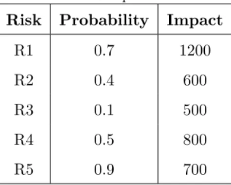
simple example to illustrate these stages and identify the main issue with adopting this process in case of interdependent risks. In the risk identification stage, specific risks must be identified. Let us assume that there are five risks namely R1, R2, R3, R4 and R5 that have been identified for a hypothetical supply chain using standard tools of checklists, risk mapping and taxonomies. In the risk assessment stage, each risk is assigned the probability and impact values and in our example, we assign arbitrary 165
values to the risks as shown in Table 1. These risks are subsequently mapped on a risk matrix for the sake of prioritisation (risk analysis) and selecting risk mitigation actions (risk treatment).
Table 1: Risk parameters.
Risk Probability Impact
R1 0.7 1200
R2 0.4 600
R3 0.1 500
R4 0.5 800
R5 0.9 700
A risk matrix is a two-dimensional plot of risks characterised by the corresponding probability and impact values. For a detailed overview of the history of risk matrix based tools and associated shortcomings, interested readers may refer to the study conducted by Duijm (2015). One of the main 170
limitations of these tools is their lack of capturing the risk attitude of a decision maker. Using utility theory, Ruan et al. (2015) introduced a three step process for integrating risk attitude in the risk matrix by: (a) describing risk attitudes of decision makers by utility functions; (b) introducing utility indifference curves and embedding these into the risk matrix; and (c) discretising utility indifference
curves. Integration of indifference curves representing the decision maker’s preferences within the 175
risk matrix results in discretising the risk matrix into five risk zones: Negligible –no need for further concern; Acceptable –need for monitoring the risks with no investment; Controllable –need for adopting emergency plans; Critical –need for mitigating risks as long as the benefits exceed the costs; and Unacceptable –need for bringing the risks down to the critical level at any cost.
The first step involves establishing the utility function of a decision maker. As opposed to the 180
concept of utility adopted in the standard expected utility approach where utility is mapped over the set of all possible outcomes, the utility function used here represents the utility of a decision maker with respect to the loss realising from an individual risk. In this example, we assume that the decision maker is risk-neutral (utility of loss [u(l)] =loss). The utility indifference curves segregate the entire risk matrix into five regions: unacceptable; critical; controllable; acceptable; and negligible risk zones 185
(Ruan et al., 2015). Therefore, we need a total of four utility indifference curves in order to establish the boundaries of these five regions as shown in Figure 1. Each indifference curve represents a particular risk level comprising a number of points with different combinations of probability and utility of loss values. Equation 4 represents a utility indifference curve where p0 and u(l0) are the probability and utility of loss values, respectively specific to a reference point on the curve (Ruan et al., 2015). 190
p∗u(l) =p0∗u(l0) (4)
Considering the reference point as having a probability of 1, Equation 4 is transformed as follows:
p∗u(l) =u(l0) (5)
The value ofu(l0) is unique for each curve and influenced by the risk appetite of a decision maker. For a detailed discussion on selecting the reference points and segregating the risk matrix into risk zones, interested readers may refer to Ruan et al. (2015). In the case of a risk-neutral decision maker, Equation 5 is reduced to:
195
p∗l=u(l0) (6)
The five zones representing relative importance of risks are unacceptable (R-I), critical (R-II), controllable (R-III), acceptable (R-IV) and negligible (R-V) as shown in Figure 1. The unacceptable zone also includes the area of the risk matrix beyond the threshold impact (in this case, above the line: impact=1500). We have assumed that 1500 is the maximum tolerance level of the decision maker beyond which a risk with any probability value must be mitigated. Each risk considered in our example 200
occupies a specific zone. The values of u(l0) (corresponding to the reference points A, B, C and D) specific to the four indifference curves are assumed as −695, −521,−347 and −174, respectively.
Figure 3: Utility indifference curves based risk matrix
As R1 is an unacceptable risk, it must be mitigated at any cost. R5 must be mitigated if the benefit exceeds the cost. We can identify a strategy or combinations of strategies that would either reduce the probability or impact of a risk or a set of risks. It is very easy to conduct the risk treatment as we only need to evaluate the benefits through executing simple arithmetic operations and weigh these against the total cost of implementing strategies. Therefore, we can prioritise risks and select optimal strategies through following a sequential risk management process. During the risk monitoring stage, any new risk(s) and/or changes in the parameters of existing risks must be incorporated in the risk matrix.
3.3. Motivation and Significance of the Research
Now let us consider that instead of a set of independent risks, we are dealing with a network of risks where there are interdependencies between risks and a risk might have a (positive or negative) correlation with another risk or a set of risks. Similarly, a mitigation strategy can have an association with multiple risks or multiple strategies can influence a single risk. Existing frameworks fail to account for evaluation and treatment of such network of risks. In the case of interdependent risks, we need to marginalise the probability values through assigning conditional probability values to the risks. Similarly, the existing risk matrix based tools are not capable of projecting the criticality of interdependent risks. Furthermore, the criterion for conducting cost-benefit analysis for the network of risks and potential strategies taking into account the risk appetite of the decision maker and linking it back to the
performance of individual risks on the risk matrix is not established. In the case of risk treatment, we can no longer rely on simple mathematical operations as each potential strategy or a combination of
R1 R2 R3 R4 R5 0 300 600 900 1200 1500 0 0.2 0.4 0.6 0.8 1 Impa ct P(Ri=True) R-I R-II R-III R-IV R-V A B C D
Figure 1: Utility indifference curves based risk matrix.
AsR1 is an unacceptable risk, it must be mitigated at any cost. R5 must be mitigated if the benefit
exceeds the cost. We can identify a strategy or combinations of strategies that would either reduce the probability or impact of a risk or a set of risks. It is very easy to conduct the risk treatment as 205
we only need to evaluate the benefits through executing simple arithmetic operations and weigh these against the total cost of implementing strategies. Therefore, we can prioritise risks and select optimal strategies through following a sequential risk management process. During the risk monitoring stage, any new risk(s) and/or changes in the parameters of existing risks must be incorporated in the risk matrix.
210
4.1. Motivation for Developing a New Process
Now let us consider that instead of a set of independent risks, we are dealing with a network of risks where there are interdependencies between risks and a risk might have a (positive or negative) correlation with another risk or a set of risks. Similarly, a mitigation strategy can have an association with multiple risks or multiple strategies can influence a single risk. Existing frameworks fail to account 215
for evaluation and treatment of such network of risks. In the case of interdependent risks, we need to marginalise the probability values through assigning conditional probability values to the risks. The existing risk matrix based tools are not capable of projecting the criticality of interdependent risks. Furthermore, the criterion for conducting cost-benefit analysis for the network of risks and potential strategies taking into account the risk appetite of a decision maker and linking it back to the 220
performance of individual risks on the risk matrix is not established. In the case of risk treatment, we can no longer rely on simple mathematical operations as each potential strategy or a combination of strategies must be linked to the risk network and the marginal probability values of risks must be re-evaluated and the resulting risks mapped again on the risk matrix. Therefore, it makes the process as iterative rather than sequential.
225
EUT being widely used in decision making under uncertainty provides a systematic approach of evaluating optimal strategies (Aven, 2015); however, even for a very simple network of 5 risks and 5
strategies, a total of 1024 values must be elicited from the decision maker with regard to the utility of different combinations of risks and strategies. Furthermore, as reported in the literature on risk management, practitioners rely on risk matrix based tools to prioritise risks (Ruan et al., 2015). 230
Therefore, we aim to propose a method through modifying the utility indifference curves based risk matrix (Ruan et al., 2015) and utilising cost-benefit analysis to prioritise supply chain risk mitigation strategies taking into account the risk appetite of a decision maker.
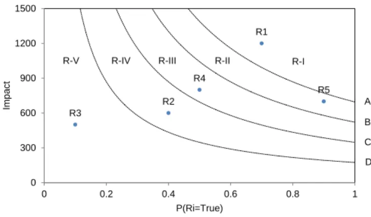
5. Proposed Risk Matrix Driven Supply Chain Risk Management Process
We adapt the established risk management framework (SA, 2009) as it is used widely both by 235
researchers and practitioners (Khan et al., 2008). Although the description of terms and concepts used in the framework is controversial (Aven, 2011), our focus is limited to the stages involved in the process. The proposed process is shown in Figure 2. Instead of treating risks in isolation, we introduce the concept by developing a risk network. The process starts with the specification of context in terms of defining the boundary of a supply chain/network and identifying the stakeholders involved in the 240
risk management process.
Risk network identification is a critical stage where there is a need for bringing a paradigm shift as the existing literature is rife with conventional tools and techniques of identifying risk categories and the concept of developing causal risk paths/risk network has gained limited attention (Garvey et al., 2015). Besides identifying the risks and risk sources, potential risk mitigation strategies must also be 245
included within the network. Risk network analysis involves determining the (conditional) probability values and loss values associated with risks subject to the implementation of specific risk mitigation strategies.
In the risk network evaluation stage, there is a need to explore new risk measures that can be computed easily and are capable of capturing the network-wide impact of risks. The measures are 250
also influenced by the risk appetite. In addition to registering the holistic impact of risks within the network setting, there is also a need for visualising the impact of each risk on the network of risks and ensuring that all risks are mitigated to the required level. Therefore, a modified risk matrix capable of evaluating interdependent risks coupled with the mapping of utility indifference curves (Ruan et al., 2015) must be developed and consulted for risk network evaluation as shown in Figure 3.
255
As the objective of our research is to introduce a risk management process for interdependent risks, we are not focusing on the techniques for establishing the risk appetite of a decision maker and mapping utility indifference curves on the modified risk matrix. The procedure proposed by Ruan et al. (2015) can be utilised for implementing the proposed process. However, we are not dealing with the discretisation of risk matrix because of the probability and loss values used in the proposed 260
Figure 4: Supply chain risk network management (SCRNM)
Risk network identification is a critical stage where there is a need for bringing a paradigm shift as the existing literature is rife with conventional tools and techniques of identifying risk categories and the concept of developing causal risk paths/risk network has gained limited attention (Badurdeen et al., 2014, Garvey et al., 2015). Besides identifying the risks and risk sources, potential risk mitigation strategies must also be included within the network. Risk network analysis involves determining the (conditional) probability values and loss values associated with risks subject to the implementation of specific risk mitigation strategies. In the risk network evaluation stage, there is a need to explore new risk measures that can be computed easily and are capable of capturing the network wide impact of risks. The measures are also influenced by the risk appetite. In addition to registering the holistic impact of risks within the network setting, there is also a need for visualising the impact of each risk on the network of risks and ensuring that all risks are mitigated to the required level. Therefore, a modified risk matrix capable of evaluating interdependent risks coupled with the mapping of utility indifference curves (Ruan et al., 2015) must be developed and consulted for risk network evaluation as shown in Figure 5.
Establishing the Context
Risk Network Identification
Risk Network Analysis
Risk Network Evaluation
Risk Network Treatment
Implementation of Strategies
Risk Network Monitoring Establishing the
Risk Appetite
Modified Risk Matrix
Figure 2: Risk matrix driven supply chain risk management (RMSCRM). As the objective of our research is to introduce a risk management process for interdependent risks, we are not focusing on the techniques for establishing the risk appetite of the decision maker and mapping utility indifference curves on the modified risk matrix. The procedure proposed by Ruan et al. (2015) can be utilised for implementing the proposed process. However, we are not dealing with the discretisation of risk matrix because of the probability and loss values used in the proposed risk management process. Appropriate risk measures representing the network wide holistic impact of risks can be used for risk analysis/evaluation and corresponding to each combination of strategies, the configuration of individual risks (R1, R2, R3, R4) can be mapped on the modified risk matrix. The matrix is bounded by the upper limit of loss beyond which a risk irrespective of its probability value must be treated.
Risk network treatment deals with the evaluation of different combinations of risk mitigation strategies within the network setting. The modified risk matrix provides a lens to evaluate the efficacy of strategies and establish if additional strategies must be implemented. The proposed process flow is in contrast with the one established in extant literature as instead of following a unidirectional flow, it is an iterative process where evaluation of each combination of strategies necessitates re-assessing and re-evaluating the risk network. The iterative process results in the selection of an optimal combination of strategies that not only considers the network wide holistic effect of these strategies but also yields an acceptable configuration of risks mapped on the modified risk matrix. The matrix also helps in identifying critical risks that must be monitored periodically. After determining the optimal combination of strategies, these are implemented and as risk management is a continuous process, there is a need for continuously monitoring risks and updating the risk network on a regular basis.
Figure 5: Mapping from risk network evaluation to modified risk matrix
R1 R2 R4 R3 0 0.2 0.4 0.6 0.8 1 Co nd itio na l lo ss P(Ri=True) Ri sk ne tw ork lo ss
Total cost of implementing mitigation strategies
risks can be used for risk analysis/evaluation and corresponding to each combination of strategies, the configuration of individual risks (R1, R2, R3, R4) can be mapped on the modified risk matrix. The matrix is bounded by the upper limit of loss beyond which a risk irrespective of its probability value must be treated.
265
Risk network treatment deals with the evaluation of different combinations of risk mitigation strate-gies within the network setting. The modified risk matrix provides a lens to evaluate the efficacy of strategies and establish if additional strategies must be implemented. The proposed process flow is in contrast with the one established in extant literature as instead of following a unidirectional flow, it is an iterative process where evaluation of each combination of strategies necessitates re-assessing and 270
re-evaluating the risk network. The iterative process results in the selection of an optimal combination of strategies that not only considers the network-wide holistic effect of these strategies but also yields an acceptable configuration of risks mapped on the modified risk matrix. The matrix also helps in identifying critical risks that must be monitored periodically. After determining the optimal combina-tion of strategies, these are implemented and as risk management is a continuous process, there is a 275
need for continuously monitoring risks and updating the risk network on a regular basis. 5.1. Proposed Approach
5.1.1. Modelling Assumptions
The model is based on the following assumptions:
• Supply chain risks, corresponding sources and potential mitigation strategies are known and these 280
can be modelled as an acyclic directed graph.
• All random variables and risk mitigation strategies are represented by binary states.
• Conditional probability values for the risks and associated losses can be elicited from the stake-holders and the resulting network represents close approximation to the actual perceived risks and interdependency between different risks.
285
• Cost associated with each potential risk mitigation strategy is known.
5.1.2. Supply Chain Risk Network
A discrete supply chain risk networkRN = (X, G, P, L, U, C) is a six-tuple consisting of:
• a directed acyclic graph (DAG),G= (V, E) , with nodes,V, representing discrete risks and risk sources,XR, discrete risk mitigation strategies, XS, and directed links, E, encoding dependence
290
relations,
• a set of conditional probability distributions, P, containing a distribution, P(XRi|Xpa(Ri)), for each risk and risk source,XRi,
• a set of loss functions, L, containing one loss function, l(Xpa(V)), for each node v in the subset
Vl∈V of loss nodes,
295
• a set of utility functions, U, containing one utility function, u(Xpa(V)), for each node v in the subsetVu ∈V of utility nodes,
• a set of cost functions, C, containing one cost function, c(Xpa(V)), for each nodev in the subset
Vc∈V of cost nodes.
Risk network expected loss,RN EL(X), is given by (Qazi et al., 2015a): 300 RN EL(X) = Y Xv∈XR P(Xv|Xpa(v)) X w∈VL l(Xpa(w)) (7)
Expected utility for loss,EU(X), is given by (Qazi et al., 2015b):
EU(X) = Y Xv∈XR P(Xv|Xpa(v)) X w∈VL u(Xpa(w)) (8)
Risk network expected utility, RN EU(X, C(XSi)) orRN EU, is given by:
RN EU =f(EU(X), C(XSi)) (9)
whereXSi is a combination of potential strategies.
5.1.3. Risk Measure
We make use of a risk measure namely Risk Network Expected Loss Propagation Measure (RN ELP M) 305
in order to evaluate the relative contribution of each supply chain risk towards the loss propagation across the entire network of risks. RN ELP M is the relative contribution of each risk factor to the propagation of loss across the entire network of supply chain risks given the scenario that the specific risk is realised (Qazi et al., 2017).
RN ELP MXRi =RN EL(X|XRi =true).P(XRi =true) (10)
5.1.4. Risk Configuration Metric 310
Risk configuration metric (RCM) represents the preference of a decision maker with regard to the configuration of risks on the modified risk matrix specific to a particular combination of available strategies represented byXSi. A pure qualitative metric focusing on the relative number of risks within each risk zone may be represented as follows:
RCMXSi =
n1.a1+n2.a2+n3.a3+n4.a4+n5.a5
whereni and ai represent the number of risks in the risk zone iand the criticality significance of
315
risk zone ion a normalised scale, respectively, N is the total number of risks.
However, we consider the following risk metric to be appropriate as defined over a range of contin-uous values:
RCMXSi =
X
XR
−u(RN ELXSi(X|XRi =true)).P(XRi)XSi (12)
Equation 11 is the discretised form of Equation 12 where each risk zone is assigned a preference 320
value and any pair of risks located in the same zone would have the same value. The main purpose of using Equation 12 is not to treat the individual utility functions of risks as mutually independent and add these together, but rather to evaluate the preference of the risk configuration specific to a combination of strategies with respect to the utility indifference curves mapped. Therefore,RCMXSi
is a preference measure to help the decision maker prioritise between two different combinations of 325
strategies with regards to the distribution of risks on the risk matrix. Unlike the expected utility approach where all possible combinations of outcomes are evaluated, we only consider the possibility that a particular risk materialises and register the impact of all risks in turn. A combination of strategies yielding an optimal aggregate value of these instantiations subject to the constraints of risk zones and cost-effectiveness is finally selected.
330
The normalised risk metric is defined as follows:
¯
RCMXSi = 1−
RCMXSi
max(RCMXS)
(13) whereRCMXS is the entire set of RCM values for all possible combinations of strategies.
5.1.5. Problem Setting
Given five zones of risk prioritisation in the modified risk matrix segregated by the utility indiffer-ence curves (pi∗u(li) =−Aj∀XRi(pi, li) on the curvej) and the threshold loss,l
∗ (defining the portion
335
of unacceptable zone represented by the area of risk matrix above that threshold line) where the set (A1, A2, A3, A4) representing constant values arranged in descending order corresponds to the set of
curves segregating the five risk zones: unacceptable; critical; controllable; acceptable; and negligible. What is the optimal set of combinations of strategies, ¯Sp = ( ¯Sp1, ...,S¯pr) with associated set of total cost of mitigation strategies C( ¯Sp) = (C( ¯Sp1), ..., C( ¯Spr)) for the entire risk network such that 340
each ¯Spi (comprising a specific combination of potential strategies) yields the (maximum) minimum value of the (normalised) risk configuration metric (RCM) subject to the risk mitigation requirements of each risk zone?
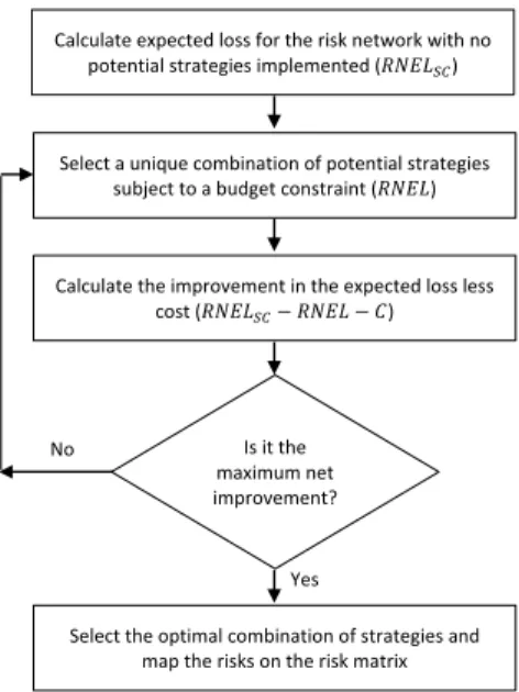
Fig. B.2. Flow chart for selecting optimal strategies specific to a risk-neutral decision maker Calculate expected loss for the risk network with no
potential strategies implemented (𝑅𝑁𝐸𝐿𝑆𝐶)
Is it the maximum net improvement?
Select a unique combination of potential strategies subject to a budget constraint (𝑅𝑁𝐸𝐿)
Yes
Calculate the improvement in the expected loss less cost (𝑅𝑁𝐸𝐿𝑆𝐶− 𝑅𝑁𝐸𝐿 − 𝐶)
Select the optimal combination of strategies and map the risks on the risk matrix No
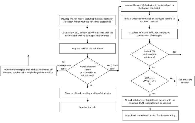
Figure 4: Flow chart for selecting optimal strategies specific to a risk-neutral decision maker.
5.1.6. Proposed Algorithms
We propose two different algorithms for managing risks corresponding to the risk-neutral and 345
risk-averse/risk-seeking decision makers as shown in Algorithm A.4 and Algorithm A.5, respectively. Although the algorithms make use of our proposed risk measure, these are still adaptable for incor-porating other risk measures. We have intentionally not included the stage of risk identification as a relevant algorithm already exists for developing the risk network (Garvey et al., 2015). The flow charts specific to Algorithm A.4 and Algorithm A.5 are shown in Fig 4 and Fig 5, respectively.
350
5.1.7. Modelling Process
The following steps must be pursued in developing a BBN based risk network of interacting supply chain risks and risk mitigation strategies:
• Define the boundaries of the supply network and identify stakeholders.
• Identify a network of key risks, corresponding risk sources and potential risk mitigation strategies 355
on the basis of input received from each stakeholder through interviews and/or focus group sessions.
• Refine the qualitative structure of the resulting network involving all stakeholders.
• Elicit (conditional) probability values, loss (utility) values resulting from risks and cost associated with implementing each potential mitigation strategy and populate the BBN with all values. 360
• Run the model and follow Algorithms A.4 and A.5 specific to a risk-neutral and risk-averse/risk-seeking decision maker, respectively for assessing and treating risks.
Fig. B.2. Flow chart for selecting optimal strategies specific to a risk-averse (seeking) decision maker Map the risks on the risk matrix
Calculate 𝑅𝑁𝐸𝐿𝑆𝐶 and 𝑅𝑁𝐸𝐿𝑃𝑀 of each risk for the
risk network with no strategies implemented
No need of implementing additional strategies
Calculate 𝑅𝐶𝑀 and 𝑅𝑁𝐸𝐿 for the specific combination of strategies
No
Develop the risk matrix capturing the risk appetite of a decision maker with five risk zones established
Select a unique combination of strategies specific to each cost selected
Is the 𝑅𝐶𝑀 evaluated the minimum? improvement? 𝑅𝑁𝐸𝐿𝑆𝐶− 𝑅𝑁𝐸𝐿 − 𝐶 > 0? Any risk located
in the unacceptable or critical zone? Yes No Yes
All such solutions are feasible and the one with the minimum 𝑅𝐶𝑀 (optimal) must be selected Yes (critical
zone)
Monitor the risks
Increase the cost of strategies (in steps) subject to the budget constraint
No Not a feasible solution Implement strategies until all risks are cleared off
the unacceptable risk zone yielding minimum 𝑅𝐶𝑀 Yes (unacceptable
zone)
Map the risks on the risk matrix for risk monitoring
Figure 5: Flow chart for selecting optimal strategies specific to a risk-averse (seeking) decision maker.
5.2. Illustrative Example: Demonstration of Key Concepts
In order to demonstrate the key concepts introduced, we present a simple network comprising five 365
risks (Ri) and four potential risk mitigation strategies (Si) as shown in Figure 6. It is assumed that each risk is associated with a loss value of 100 units and each strategy can be implemented at a cost of 30 units. Each risk is considered to have binary states: True (T) or False (F). Similarly, each mitigation strategy is assumed to be in one of the binary states: Yes (Y) or No (N). The (conditional) probability values are shown in Table A.1. The shaded cells represent the (conditional) probability values once 370
the corresponding mitigation strategy is selected. It is interesting to consider positive correlation of S1 with R2.
5.2.1. Risk-Neutral Decision Maker
A risk-neutral decision maker interested in maximising reduction in the cost adjusted risk network expected loss does not account for the relative importance of each risk in terms of its relative position 375
on the modified risk matrix. The decision maker would only select a combination of strategies and make an investment if there is an increase in the reduction of risk network expected loss less cost. Under the standard configuration, the risks are evaluated with respect to the existing strategies once none of the potential strategies are selected. All possible combinations of potential strategies (S1,S2,
S3,S4) are shown in Table A.2.
shown in Table 8 (refer to the Appendix). The shaded cells represent the (conditional) probability values once the corresponding mitigation strategy is selected. It is interesting to consider positive correlation of S1 with R2.
Figure 6: Risk network modelled in GeNIe (GeNIe, 2015)
5.3.1. Risk-Neutral Decision Maker
A risk-neutral decision maker interested in maximising reduction in the risk network expected loss less cost does not account for the relative importance of each risk in terms of its relative position on the modified risk matrix. The decision maker would only select a combination of strategies and make an investment if there is an increase in the reduction of risk network expected loss less cost. Under standard configuration, the risks are evaluated with respect to the existing strategies whereas none of the potential strategies is selected. All possible combinations of potential strategies (S1, S2, S3, S4) are shown in Table 4.
Table 4: Combinations of risk mitigation strategies
Combination of Risk Mitigation Strategies Risk Mitigation Strategies Total Cost S - 0 A S2 30 B S4 30 C S3 30 D S1 30 E S2, S4 60 F S2, S3 60 G S3, S4 60 H S1, S2 60 I S1, S4 60 J S1, S3 60 K S2, S3, S4 90 L S1, S2, S4 90
Figure 6: Risk network modelled in GeNIe.
M S1, S2, S3 90
N S1, S3, S4 90
O S1, S2, S3, S4 120
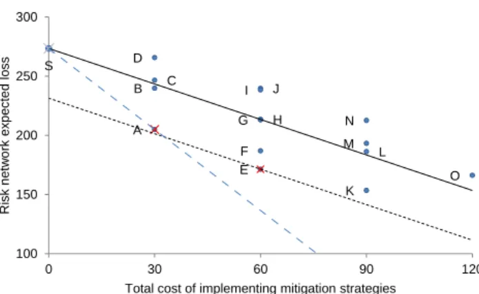
The relative performance of each combination of strategies is mapped in Figure 7. Each point represents a particular combination of strategies with corresponding cost and risk network expected loss. The solid line represents the threshold where the reduction in risk network expected loss is just equal to the cost of implementing strategies. The points (above) below this line represent all such combinations which are (in)feasible.
Figure 7: Identification of optimal combinations of strategies
The dotted line in black contains the optimal solution (point E) yielding maximum reduction in the network expected loss less cost whereas the dashed line in blue contains the optimal solution (point A) following the criterion of maximising benefit to cost ratio. Although point K is a feasible solution, it is not optimal as it fails to yield a greater reduction in network expected loss less cost relative to that of point E. A red cross represents an optimal solution. The decision maker will select point A if the available budget is less than 60 units but at least 30 units whereas for budget greater than and inclusive of 60 units, point E is the optimal solution.
5.3.2. Risk-Averse Decision Maker
In case of risk-averse decision maker, we assumed the utility function as represented by Equation (17).
We also assumed that the upper threshold for the loss value is 500 units. Similarly, the selected
values corresponding to the four utility indifference curves are -200, -150, -100 and -50, respectively. A C F K S B D E G H I J L M N O 100 150 200 250 300 0 30 60 90 120 Ri sk ne tw ork ex pe cted lo ss
Total cost of implementing mitigation strategies
Figure 7: Identification of optimal combinations of strategies.
The relative performance of each combination of strategies is mapped in Figure 7. Each point represents a particular combination of strategies with corresponding cost and risk network expected loss. The solid line represents the threshold where the reduction in risk network expected loss is just equal to the cost of implementing strategies. The points (above) below this line represent all such combinations which are (in)feasible.
385
The dotted line contains the optimal solution (point E) yielding maximum reduction in the network expected loss less cost whereas the dashed line contains the optimal solution (point A) following the criterion of maximising benefit to cost ratio. Although point K is a feasible solution, it is not optimal as it fails to yield a greater reduction in the cost adjusted network expected loss relative to that of point E. A cross represents an optimal solution. The decision maker will select point A if the available 390
budget is less than 60 units but at least 30 units whereas for a budget greater than and inclusive of 60 units, point E is the optimal solution.
5.2.2. Risk-Averse Decision Maker
In the case of a risk-averse decision maker, we assume the utility function as represented by Equation 14. We also assume that the upper threshold for the loss value is 500 units. Similarly, the selectedu(l0) 395
Figure 8: Normalised expected utility for loss corresponding to various strategies
Figure 9: Risk network expected utility as summation of independent utilities
Table 5: Optimal solutions for the objective function of maximising
Combination of Risk
Mitigation Strategies Cost of Strategies
A E K A C F K B D E G H I J L M N O S 0 0.2 0.4 0.6 0.8 1 0 30 60 90 120 Ex pe cted util ity for lo ss
Total cost of implementing mitigation strategies
A C F K S B D E G H I J L M N O 0 5000 10000 15000 20000 25000 30000 35000 0 30 60 90 120 Ri sk ne tw ork ex pe cted di sutil ity
Total cost of implementing mitigation strategies
Figure 8: Expected utility for loss corresponding to various strategies.
values corresponding to the four utility indifference curves are−200,−150,−100 and−50, respectively.
u(l) =−(l)2 (14)
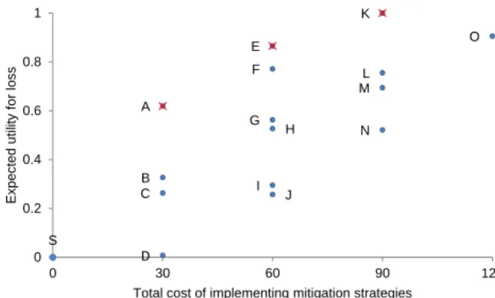
Maximising Risk Network Expected Utility. There are two ways of evaluating the risk network expected utility. We can either combine the cost of strategies and loss associated with different combinations of risks and strategies, or evaluate utility of loss and utility of cost separately and combine these together using an appropriate function and a consistent scale. The first approach needs an input of 512 values 400
as it is not possible to aggregate the individual utility values because of utility being a non-linear function in this example. Using the second approach, we can calculate the expected utility value for loss corresponding to different strategies needing only 32 values as shown in Figure 8. Points A, E and K are the optimal combinations of strategies considering expected utility for loss, however, selection of optimal strategies corresponding to risk network expected utility (function of loss and cost) depends 405
on the relative importance of expected utility for loss (w) and utility for cost (1−w) as shown in Equation 15. Importantly, the scales used for the two functions must be consistent. Point O can never be an optimal solution under any preference setting.
RN EU =w.EU(X) + (1−w).f(C(XSi)) (15)
If we assume the individual utility functions to be independent, we can use Equation 16 (Keeney & Raiffa, 1993) to calculate the overall utility for the network:
410 U(A) = n X i=1 ci.Ui(Ai) (16)
whereA is a set ofnattributes assumed as mutually utility independent, Ui(Ai) is the conditional utility for attributeAi, and
Maximising Normalised Risk Configuration Metric subject to Constraints
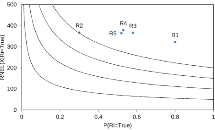
We mapped the risks corresponding to the standard configuration of network as shown in Figure 10. It can be seen that all risks are located in the unacceptable zone. Next, we evaluated the normalised risk configuration metric for all combinations of strategies as shown in Figure 11. As there are risks located in the unacceptable zone, the constraint of risk network expected loss can be ignored. Therefore, point A is the optimal solution corresponding to the cost of 30 units.
Figure 10: Risk network evaluation under standard configuration (Point S)
Figure 11: Identification of optimal solutions R1 R2 R4 R3 R5 0 100 200 300 400 500 0 0.2 0.4 0.6 0.8 1 RN EL (X |Ri =T rue ) P(Ri=True) S A C F B D E G H I J K L M N O 0 0.2 0.4 0.6 0.8 0 30 60 90 120 No rmal ise d risk con figu ratio n metric
Total cost of implementing mitigation strategies
Figure 9: Risk network evaluation under standard configuration (Point S).
Maximising Normalised Risk Configuration Metric subject to Constraints
We mapped the risks corresponding to the standard configuration of network as shown in Figure 10. It can be seen that all risks are located in the unacceptable zone. Next, we evaluated the normalised risk configuration metric for all combinations of strategies as shown in Figure 11. As there are risks located in the unacceptable zone, the constraint of risk network expected loss can be ignored. Therefore, point A is the optimal solution corresponding to the cost of 30 units.
Figure 10: Risk network evaluation under standard configuration (Point S)
Figure 11: Identification of optimal solutions R1 R2 R4 R3 R5 0 100 200 300 400 500 0 0.2 0.4 0.6 0.8 1 RN EL (X |Ri =T rue ) P(Ri=True) S A C F B D E G H I J K L M N O 0 0.2 0.4 0.6 0.8 0 30 60 90 120 No rmal ise d risk con figu ratio n metric
Total cost of implementing mitigation strategies
Figure 10: Identification of optimal solutions.
Maximising Normalised Risk Configuration Metric subject to Constraints (related to the Risk Zones). We mapped the risks corresponding to the standard configuration of the network as shown in Figure 9. 415
It can be seen that all risks are located in the unacceptable zone. Next, we evaluated the normalised risk configuration metric for all combinations of strategies as shown in Figure 10. As there are risks located in the unacceptable zone, the constraint of benefit exceeding the cost can be ignored. Therefore, point A is the optimal solution corresponding to the cost of 30 units.
The risk configuration corresponding to point A is shown as Figure A.1. As two risks are still 420
in the unacceptable region, we can ignore the constraint of benefit-exceeding cost, however, point E yields the best value corresponding to both criteria (maximising normalised RCM and minimising
RN EL+cost). The risk configuration relative to point E is shown in Figure A.2. There is no risk
in the unacceptable region whereas two risks are located in the critical region. Therefore, point K is the only feasible solution as the benefit must exceed costs for further investment as shown in Figure 425
7. As point K yields higher value for normalised RCM relative to that of point E, point K is the optimal solution for budget greater than or equal to 90 units with configuration of risks shown as Figure A.3. Point O is not a feasible solution to be considered for optimality. A cross represents an optimal solution. Optimal solutions corresponding to different cost regimes are presented in Table 2.
Figure 8: Normalised expected utility for loss corresponding to various strategies
Figure 9: Risk network expected utility as summation of independent utilities
Table 5: Optimal solutions for the objective function of maximising
Combination of Risk
Mitigation Strategies Cost of Strategies
A E K A C F K B D E G H I J L M N O S 0 0.2 0.4 0.6 0.8 1 0 30 60 90 120 Ri sk ne tw ork ex pe cted util ity for lo ss
Total cost of implementing mitigation strategies
A C F K S B D E G H I J L M N O 0 5000 10000 15000 20000 25000 30000 35000 0 30 60 90 120 Ri sk ne tw ork ex pe cted di sutil ity
Total cost of implementing mitigation strategies
Table 2: Optimal solutions for the objective function of maximising normalised RCM.
6. Simulation Study
430
An application of the proposed method is demonstrated through a simple supply chain risk network (Garvey et al., 2015) as shown in Figure 11. The supply network comprises one raw material source, two manufacturers, one warehouse and one retailer. Supply chain elements, associated risks and loss values are shown in Table A.3. Although each domain of the supply network may comprise a number of risks and corresponding sources, we consider limited risks for the sake of simplicity. Each risk and 435
mitigation strategy is represented by binary states of True (T) or False (F) and Yes (Y) or No (N), respectively. Assumed (conditional) probability values are shown in Table A.4 and the effectiveness of risk mitigation strategies is represented by values appearing in the shaded cells. Potential mitigation strategies, associated risks and costs are depicted in Table A.5.
6.1. Results 440
It is assumed that the decision maker is risk-neutral. As six potential mitigation strategies were considered for implementation, a total of 64 different combinations of strategies were evaluated as shown in Figure 12. All the points below the solid line represent solutions for which the improvement in risk network expected loss is more than the cost of implementing strategies. Only points A (S6) and B (S1, S6) are the optimal solutions as all other points in the feasible region (below the solid line) fail 445
to meet the other constraint. Therefore, if the decision maker is only concerned about maximising the reduction in cost adjusted risk network expected loss, an amount of 100 units must be invested for a budget range between 100 and 200 units whereas only the strategies amounting to 200 units must be implemented for a budget regime of 200 units and more. The main problem with implementing these optimal solutions is their exclusive focus on the network wide expected loss without accounting for the 450
stra teg y is r e presente d by binary states o f ‘True (T ) o r False (F)’ a n d ‘Yes (Y) or No (N)’, resp ect ively . Ass umed (c o nditi o nal ) pro bability va lue s ar e show n in Tabl e 9 (ref er t o the App endix) an d th e effect ive ness o f risk mi tiga tion strate gie s is represen ted by values appearing in the sha ded cells. Po tent ial mit igation strate gies, as so ciate d risks an d co sts are depi ct ed in Table 7 . Figure 15 : Su pply chain risk n e twork m o delled in GeNIe (GeNIe, 2015 , Garvey e t al., 201 5 ) Table 6 : Sup p ly c hai n e le m ents, risks an d loss values Su p ply Chai n El em ent Risk Loss Raw M ateri al S ource (RM) Contaminatio n ( R 1) 200 Delay i n Shipm ent (R 2) 400 Manufac turer -I ( M 1) Machi ne Failur e (R4) 200 Delay i n Shipm ent (R 5) 400 Manufac turer -II (M2) Machi ne Failur e (R3) 200 Delay i n Shipm ent (R 6) 400 Wareho use (W) Overbur dene d E mpl o yee (R7) Damage to Inventory (R8 ) 500 Delay i n Shipm ent (R 9) 600 Flood (R 12) Wareho use to Retail er ( W -R) Tr uc k Accide nt ( R 10) 500 Retail er ( R) Inventory S hor tage (R11 ) 800
Figure 11: A supply chain risk network modelled in GeNIe (Source: Garvey et al. 2015). Table 7: Potential risk mitigation strategies, associated risks and cost
Risk Mitigation
Strategy Description Associated Risk Cost
S1 Quality Assurance Program R1 100
S2 Scheduled Maintenance Program R3 50
S3 Scheduled Maintenance Program R4 100
S4 Scheduling Software and Monitoring
Program R7 50
S5 Early Warning System R8 200
S6 Training Simulator R10 100
6.1. Results
We assumed that the decision maker is risk-neutral. As six potential mitigation strategies were considered for implementation, a total of 64 different combinations of strategies were evaluated as shown in Figure 16. All the points below the solid line represent solutions for which the improvement in risk network expected loss is more than the cost of implementing strategies. Only points A (S6) and B (S1, S6) are the optimal solutions as all other points in the feasible region (below the solid line) fail to meet the other constraint. Therefore, if the decision maker is only concerned about maximising the reduction in risk network expected loss less cost, an amount of 100 units must be invested for a budget range of 100-200 (exclusive) units whereas only the strategies amounting to 200 units must be implemented for a budget regime of 200 units and more. The main problem with implementing these optimal solutions is their exclusive focus on the network wide expected loss without accounting for the configuration of risks corresponding to other feasible solutions.
Figure 16: Identification of optimal combinations of strategies S A B 1200 1400 1600 1800 0 100 200 300 400 500 600 Ri sk ne tw ork ex pe cted lo ss
Total cost of implementing mitigation strategies
7. Second Approach for Selecting Optimal Strategies (Without Using the Risk Matrix)
In this approach, a different line of inquiry is adopted where the decision maker utilises the informa-tion about cost of strategies and the impact of strategies on the risk exposure (risk network expected loss) to select a portfolio of optimal strategies. With reference to the risk network modelled in Figure 455
11, all possible combinations of strategies are mapped again in Figure 13; however, here we distinguish between the set of Pareto-optimal solutions (non-dominated solutions) and the dominated solutions specific to different budget constraints that are represented by filled and hollow circles, respectively. The definition of Pareto-optimal set introduced by Spackova & Straub (2015) is adopted that contains all such combinations of strategies for which there are no other combinations that have simultaneously 460
lower costs and lower risk exposure. Points O and P are included in the set of Pareto-optimal solutions; however, for a risk-neutral decision maker, these points fall short of the threshold criterion demanding the equivalence of improvement in risk exposure and the additional investment. For each budget con-straint, the point is selected which maximises the perpendicular distance between the solid line and the parallel family of lines. Therefore, for a budget lesser than 200 units, point A is the optimal mix 465
of strategies whereas for all other budget constraints, point B is the optimal solution.
In contrast to a risk-neutral decision maker, a risk-averse individual would have greater concern with regards to the occurrence of risks and therefore, they will prefer to avoid such situations at the cost of enhanced investment. The risk appetite of a risk-averse individual can be modelled through a line with lower gradient (like the solid blue line in Figure 14) which indicates that the individual is 470
willing to invest relatively more than the risk-neutral individual to achieve same reduction in the risk exposure. Similarly, a risk-seeking individual represented by the red line as shown in Figure 14 (with a steeper gradient) would only be willing to invest if the improvement in risk exposure is more than the figure determined through the cost-benefit analysis.
For the blue line, all the solutions included in the Pareto-optimal set are feasible solutions. Depend-475
ing on the gradient of the line, different points will be optimal subject to the budget constraint. Once
7. Second Approach to Selecting Optimal Strategies (without using the Risk Matrix)
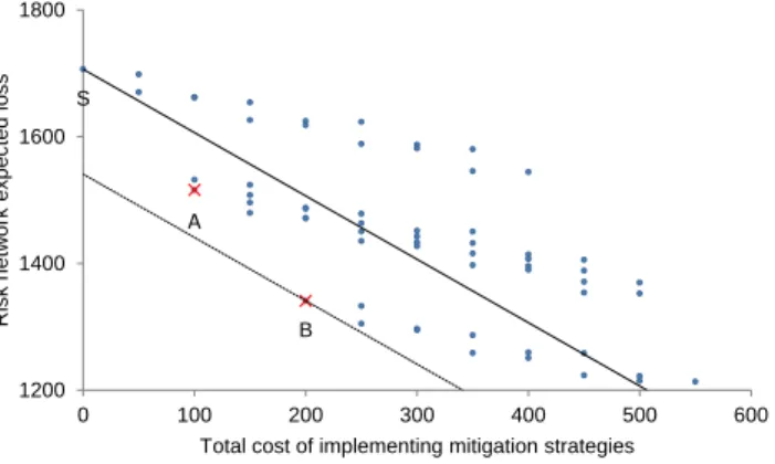
In this approach, we focus on a different line of inquiry where the decision maker utilises the information about cost of strategies and the impact of strategies on the risk exposure (risk network expected loss) to select a portfolio of optimal strategies. With reference to the risk network modelled in Figure 15., all possible combinations of strategies are mapped again in Figure 17; however, here we distinguish between the set of Pareto optimal solutions (non-dominated solutions) and the dominated solutions specific to different budget constraints that are represented by filled and blank circles, respectively. We adopt the definition of Pareto optimal set (Špačková and Straub, 2015) to contain all such combinations of strategies for which there are no other combinations that have simultaneously lower costs and lower risk exposure. Points O and P are included in the set of Pareto optimal solutions; however, for a risk-neutral decision maker, these points fall short of the threshold criterion demanding the equivalence of improvement in risk exposure and the additional investment. For each budget constraint, the point is selected which maximises the perpendicular distance between the solid line and the parallel family of lines. Therefore, for a budget lesser than 200 units, point A is the optimal mix of strategies whereas for all other budget constraints, point G is the optimal solution.
Figure 17: Pareto optimal solutions (filled circles) and dominated solutions (hollow circles) In contrast to a risk-neutral decision maker, a risk-averse individual would have greater concern with regards to the occurrence of risks and therefore, he will prefer to avoid such situations at the cost of enhanced investment. The risk appetite of a risk-averse individual can be modelled through a line with lower gradient (like the solid blue line in Figure 18) which indicates that the individual is willing to invest
S A B C J K L M N O P 1200 1400 1600 1800 0 100 200 300 400 500 600 Risk network expected los s
Total cost of implementing mitigation strategies
neutral decision maker will be indifferent between and . However, the risk-averse individual will
consider the significance of in reducing the loss value far greater than the increase in investment
mainly because the loss values associated with different scenarios might be deleterious to his business.
Similarly, a risk-seeking individual would want a greater margin of improvement in with respect to
the same investment made. For the same improvement in from 1600 to 1500 units as shown in
Figure 18, the risk-seeking individual is willing to invest 50 units whereas the risk-neutral (averse) individual would invest 100 (240) units.
Figure 18: Family of lines representing risk appetite influencing the set of feasible solutions In order to combine the cost of strategies and associated risk exposure, we need to adopt a consistent method of mapping these together on a single scale. For each combination of strategies, we register the improvement in risk exposure and reduction in mitigation cost (negative of cost) with respect to the current configuration of strategies already implemented. We suggest using the method of ‘swing weights’ (Belton and Stewart, 2002) to determine the relative weight of the two criteria where the
decision maker is asked to consider that both improvement in and reduction in mitigation cost are
at the least preferred states (all risks realised and maximum possible cost of strategies incurred each amounting to the value of 0). Subsequently, he is given a scenario that only one of these could be improved to the best possible state and the one picked by him should receive the maximum weight (100) reflecting the significance of that criterion. He is then required to assess the overall value (over a scale of 0-100) arising from a swing from 0 (worst state) to 1 (best state) on the other criterion corresponding to
S A B C J K L M N O P 1200 1300 1400 1500 1600 1700 1800 0 50 100 150 200 250 300 350 400 450 500 550 600 Risk network expected los s
Total cost of implementing mitigation strategies
Figure 14: Family of lines representing risk appetite influencing the set of feasible solutions.
the line approaches a gradient of zero, all points will be optimal solutions subject to the respective budget constraint meaning that point P will be picked for a budget of at least 550 units and similarly, point O for a budget of at least 500 units but lesser than 550 units. For the red line mapped, it is evident that only point A is the optimal solution for a budget of at least 100 units.
480
Another approach to justifying the relevance of trade-off between the improvement in risk exposure and the additional investment specific to the risk appetite is illustrated through a simple example. With reference to Figure 13, a point represents a specific combination of strategies with associated cost and risk exposure across the risk network shown in Figure 11. Risk exposure across the 12 risk events can be represented as:
485
RN EL=P( ¯R1∩R¯2...R¯12).L( ¯R1∩R¯2...R¯12)...+P(R1∩R2...R12).L(R1∩R2...R12) (17)
WhereP( ¯Ri) andL(Ri) represent probability of riskRi not happening and the loss associated with
the occurrence of risk Ri, respectively.
RN EL=P( ¯R).0 +P(R).L(e R)e (18)
Where ¯Ris a scenario of no risk realising and Rerepresents a scenario of at least one risk realising.
RN EL=P(R).L(e R)e (19)
The improvement in RN EL subject to an additional investment helps in reducing the value of
P(R) and/ore L(R). For a risk-neutral decision maker, the improvement ine RN EL must be equal
490
to the additional investment at the minimum. However, the loss value (L(R)) might have reducede by a greater margin in comparison with the change in investment. For example, if a combination of strategies X[Y] yields P(R) ande L(R) values of 0.2[0.2] and 100[200], respectively at a cost of 70[50]e units, the risk-neutral decision maker will be indifferent between X and Y. However, the risk-averse individual will consider the significance of X in reducing the loss value far greater than the increase 495
in investment mainly because the loss values associated with different scenarios might be deleterious to their business. Similarly, a risk-seeking individual would want a greater margin of improvement in
RN EL with respect to the same investment made. For the same improvement in RN ELfrom 1600
to 1500 units as shown in Figure 14, the risk-seeking individual is willing to invest 50 units whereas the risk-neutral (averse) individual would invest 100(240) units.
500
In order to combine the cost of strategies and associated risk exposure, there is a need to adopt a consistent method of mapping these together on a single scale. For each combination of strategies, we register the improvement in risk exposure and reduction in mitigation cost (negative of cost) with respect to the current configuration of strategies already implemented. It is proposed to use the method of ‘swing weights’ (Belton & Stewart, 2002) to determine the relative weight of the two criteria 505
where the decision maker is asked to consider that both improvement in risk exposure and reduction in mitigation cost are at the least preferred states (all risks realised and maximum possible cost of strategies incurred each amounting to the value of 0). Subsequently, they are given a scenario that only one of these could be improved to the best possible state and the one picked by them should receive the maximum weight (100) reflecting the significance of that criterion. They are then required 510
to assess the overall value (over a scale from 0 to 100) arising from a swing from 0 (worst state) to 1 (best state) on the other criterion corresponding to the swing from 0 to 1 on the criterion already prioritised. The weights assigned can be normalised to add up to 1. We defineβ as the weighted sum of improvement in RN ELand reduction in mitigation cost:
β= (1−a)(improvement inRN EL) +a(reduction in mitigation cost) (20)
Where a is a parameter that captures the importance of cost as to how a decision maker may 515
place greater or lower weight on the cost of risk mitigation; when a = 0, the decision maker is not concerned about the cost of implementing strategies while in the case of a= 1, they will not consider implementing any additional strategy as the reduction in mitigation cost will be maximum at the current configuration of strategies.
For a risk-neutral decision maker, a = 0.5 because they want to get the improvement in RN EL 520
to be equal to the additional mitigation cost at the minimum and therefore, β = 0 would represent the threshold where they are willing to invest an additional amount in order to reduce risk exposure. Increasing values of β would yield a family of lines where the optimal solution subject to a budget constraint would be tangent to the line with the highest β. For a risk-averse (seeking) individual, a will be smaller (greater) than 0.5 and β>0 would generate the corresponding family of lines.
525
Equations of three solid lines shown in Figure 14 can be deduced from Equation 20 as follows: