Technological University Dublin Technological University Dublin
ARROW@TU Dublin
ARROW@TU Dublin
Dissertations School of Computing
2018
Classification Using Association Rules
Classification Using Association Rules
Colin KaneTechnological University Dublin
Follow this and additional works at: https://arrow.tudublin.ie/scschcomdis Part of the Computer Sciences Commons
Recommended Citation Recommended Citation
Kane, Colin (2018). Classification using association rules. Masters dissertation, DIT, 2018.
This Dissertation is brought to you for free and open access by the School of Computing at ARROW@TU Dublin. It has been accepted for inclusion in Dissertations by an authorized administrator of ARROW@TU Dublin. For more information, please contact
[email protected], [email protected], [email protected].
This work is licensed under a Creative Commons Attribution-Noncommercial-Share Alike 3.0 License
Classification Using Association Rules
Colin Kane
i
Declaration of Authorship
I, Colin Kane certify that this dissertation which I now submit for examination for the award of MSc in Computing (Data Analytics), is entirely my own work and has not been taken from the work of others save and to the extent that such work has been cited and acknowledged within the text of my work.
This dissertation was prepared according to the regulations for postgraduate study of the Dublin Institute of Technology and has not been submitted in whole or part for an award in any other Institute or University.
The work reported on in this dissertation conforms to the principles and requirements of the Institutes guidelines for ethics in research.
Signed: _________________________________
ii
Abstract
This research investigates the use of an unsupervised learning technique, association rules, to make class predictions. The use of association rules to make class predictions is a growing area of focus within data mining research. The research to date has focused predominately on balanced datasets or synthetized imbalanced datasets. There have been concerns raised that the algorithms using association rules to make classifications do not perform well on imbalanced datasets.
This research comprehensively evaluates the accuracy of a number of association rule classifiers in predicting home loan sales in an Irish retail banking context. The experiments designed test three associative classifier algorithms CBA, CMAR and SPARCCC against two benchmark algorithms conditional inference trees and random forests on a naturally imbalanced dataset.
The experiments implemented and evaluated show that the benchmark tree based algorithms conditional inference trees and random forests outperform the associative classifier models across a range of balanced accuracy measures. This research contributes to the growing body of research in extending association rules to make class predictions.
Key words: association rule, associative classifiers, Apriori, predictive analytics, KDD, data mining, unsupervised learning
iii
Acknowledgments
Thanks to my wife, Sarah, for giving me so much support throughout the full MSc course. She has kept my spirits up at all time.
Sincere thanks to my Supervisor, Brian Leahy, for the help and encouragement he provided to me in this project.
Thanks to my father, Martin, for helping with the proof reading and general support throughout the course.
iv
Contents
Declaration of Authorship i
Abstract ii
Acknowledgements iii
List of Figures vii List of Tables ix
Abbreviations x 1. INTRODUCTION ... 1
1.1 Overview of Research Area ... 1
1.2 Background ... 2
1.3 Research Problem ... 3
1.4 Research Objectives... 4
1.5 Research Methodologies ... 5
1.6 Scope and Limitations ... 6
1.7 Document Outline ... 7
2 LITERATURE REVIEW AND RELATED WORK ... 8
2.1 Introduction... 8
2.2 Knowledge Discovery in Databases (KDD) and Data Mining ... 9
2.3 Association Rule Learning ... 14
2.3.1 AIS Algorithm ... 17
2.3.2 Apriori Algorithm ... 17
2.3.3 Partition Algorithm ... 18
2.3.4 Frequent Pattern (FP) Growth Algorithm ... 19
2.3.5 Equivalent Class Transformation Algorithm ... 21
2.3.6 Conclusion Association Rule Learning Algorithms ... 22
2.4 Extending Association Rules to make predictions ... 24
v
2.4.2 Data Storage CR-tree representation ... 27
2.4.3 Pruning ... 27
2.4.4 Using rules to make classifications ... 32
2.5 The impact of class imbalance on Association Rules and the SPARCCC algorithm ... 34
2.6 Data Discretisation Approaches ... 40
2.7 Benchmark models ... 41
2.8 Model Validation Methods ... 43
2.9 Model Performance Metrics ... 47
2.10 Conclusion ... 51
3. DESIGN AND METHODOLOGY... 53
3.1 Introduction... 53
3.2 Data sources and creation of the ABT ... 54
3.2.1 Data Acquisition and Integration ... 54
3.2.2 Data Analysis ... 59
3.3 Software ... 61
3.4 Benchmark Models ... 62
3.4.1 Experiment 1 - Conditional Inference Trees ... 62
3.4.2 Experiment 2 - Random Forests ... 63
3.5 Classification Using Association Rule Models ... 63
3.5.1 Experiment 3 - CBA ... 63
3.5.2 Experiment 4 - CMAR ... 64
3.5.3 Experiment 5 - SPARCCC ... 68
3.6 Model Evaluation... 70
3.7 Conclusion ... 70
4. IMPLEMENTATION AND RESULTS ... 72
4.1 Introduction... 72
4.2 Benchmark models ... 72
4.3 Experiment 3 - CBA Algorithm ... 79
4.4 Experiment 4 - CMAR... 81 4.5 Experiment 5 - SPARCCC ... 83 4.6 Conclusion ... 85 5. EVALUATION ... 86 5.1 Introduction... 86 5.2 Evaluation of Experiments ... 86
vi
5.3 How these results support real-world experiments ... 91
5.4 Software Evaluation... 92
5.5 Conclusion ... 93
6. CONCLUSION ... 95
6.1 Introduction... 95
6.2 Research Definition and Research Overview ... 95
6.3 Experimentation, Evaluation and Results ... 96
6.4 Contributions to Body of Knowledge and Achievements ... 97
6.5 Future Work and Research ... 98
6.6 Conclusion ... 98
Bibliography ... 99
vii
List of Figures
Figure 2.1: Overview of the KDD Process ... 10
Figure 2.2: CRISP-DM Data Mining Process Model ... 11
Figure 2.3: Lattice for I = {1,2,3,4}... 16
Figure 2.4: FP Tree for 10 Transactions Dataset ... 20
Figure 2.5: Example of tid-list intersection ... 21
Figure 2.6: Comparison of association rule algorithms across varying support levels 23 Figure 2.7: Comparison of association rule algorithms across varying itemset densities ... 23
Figure 2.8: Example of the compression capability of CR-tree ... 28
Figure 2.9: Pruning using database coverage. ... 30
Figure 2.10: CBA Pruning Process ... 31
Figure 2.11: Chi-Squared rule choice illustration... 34
Figure 2.12: Contingency tables for Fisher’s Exact Test ... 38
Figure 2.13: Example of unsupervised data discretisation techniques ... 40
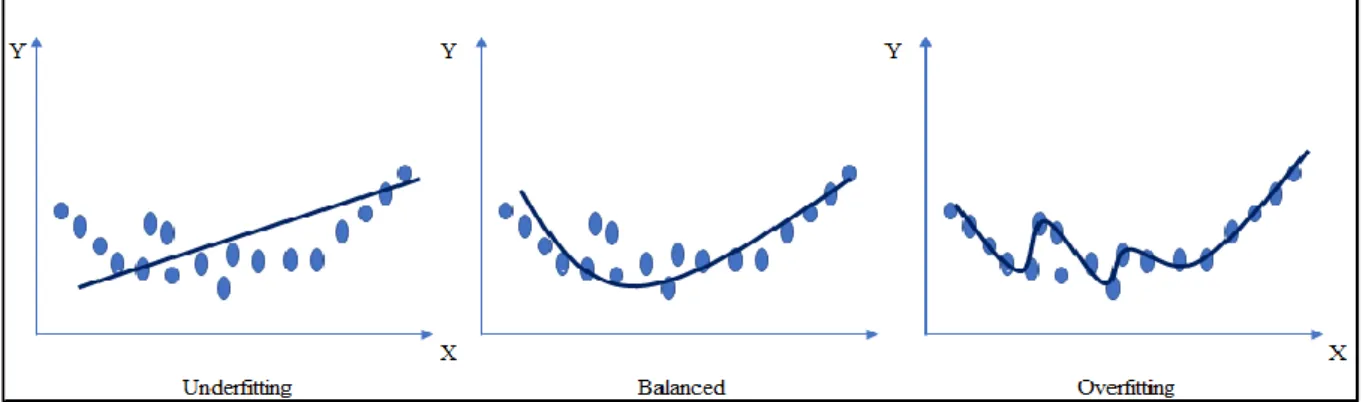
Figure 2.14: Graphical illustration of underfitting and overfitting ... 44
Figure 2.15: Illustration of the Dataset split data validation technique ... 44
Figure 2.16: K-fold Cross-Validation illustration ... 45
Figure 2.17: Example of a confusion matrix ... 47
Figure 2.18: Generic confusion matrix and key metrics... 48
Figure 2.19: Example mortgage sales confusion matrix ... 50
Figure 2.20: Calculation example Key performance metrics ... 50
Figure 3.1: Types of data available in Retail Banks ... 54
Figure 3.2: Word cloud of high frequency words from text analysis ... 58
Figure 3.3: First view of imbalance in the dataset ... 59
Figure 3.4: Response rates of particular customer segments ... 60
Figure 3.5: Dataset imbalance following first filter application ... 60
Figure 3.6: Final dataset imbalance ... 60
Figure 3.7: Dataset prior to discretisation... 66
Figure 3.8: Dataset post discretisation ... 66
Figure 3.9: GUI for data discretisation and normalisation software ... 67
Figure 3.10: GUI for WEKA used to run SPARCCC ... 69
viii
Figure 4.1: ROC for Conditional Inference Trees ... 74
Figure 4.2: Variable importance for Conditional Inference Trees ... 75
Figure 4.3: ROC comparison for Conditional Inference Trees and Random Forests .. 77
Figure 4.4: Variable Importance for Random Forests ... 78
Figure 4.5: Top ranking rules for CBA implementation ... 79
Figure 4.6: Top ranking rules for CMAR implementation ... 82
Figure 4.7: Experiment Results CMAR... 82
Figure 4.8: Subset of the rules from SPARCCC training ... 83
Figure 5.1: Top performing model across key performance metrics... 87
Figure 5.2: Top ranking rules from CMAR training ... 89
ix
List of Tables
Table 2.1: Comparison of KDD, SEMMA and CRISP-DM ... 12
Table 2.2: Sample Dataset for Supervised Learning ... 13
Table 3.1: Sample of features built from structured data ... 56
Table 3.2: Sample of features built from semi-structured data ... 56
Table 3.3: Example of data from text analysis ... 58
Table 3.4: Sample of features built from unstructured data ... 58
Table 3.5: Example data following data pre-processing for CMAR ... 65
Table 4.1: Confusion Matrix for Conditional Inference Trees ... 73
Table 4.2: Key Evaluation Metrics for Conditional Inference Trees ... 73
Table 4.3: Confusion Matrix for Random Forests ... 76
Table 4.4: Key Evaluation Metrics for Random Forests ... 76
Table 4.5: Comparison between CI Trees and Random Forests across performance metrics... 78
Table 4.6: Confusion Matrix for CBA ... 80
Table 4.7: Key Evaluation Metrics for CBA ... 80
Table 4.8: Comparison between CI Trees, Random Forests and CBA across performance metrics ... 81
Table 4.9: Confusion Matrix for SPARCCC ... 84
Table 4.10: Key Evaluation Metrics for SPARCCC ... 84
x
Abbreviations
ABT Analytics Base Table
AUC Area Under the Curve
BOI Bank of Ireland
CAR Classification Association Rules
CCR Class Correlation Ratio
CMAR Classification Based on Multiple Association Rules
CBA Classification Based Association Rules
CRM Customer Relationship Management
CRISP-DM Cross Industry Process for Data Mining
CRM Customer Relationship Management
CPU Computer Processing Unit
EDW Enterprise Data Warehouse
FN False Negative
FP False Positive
GDPR General Data Protection Regulation
GNU GNU's not Unix
I/O Input / Output
JSON JavaScript Object Notation
LOOCV Leave-one-out cross-validation
KDD Knowledge Discovery in Databases
PER Pessimistic Error Rate
R The R Project for Statistical Computing
ROC Receiver Operating Characteristic
SEMMA Sample, Explore, Modify, Model and Assess
SMOTE Synthetic Minority Oversampling Technique
SPARCCC Significant, Positively Associated and Relatively Class
Correlated Classification
SQL Structured Query Language
TN True Negative
TP True Positive
SAS Statistical Analysis System
1
1.
INTRODUCTION
1.1 Overview of Research Area
Customer expectations of their retail banking experiences are growing. As customers receive a greater level of personalised customer experience across many of their daily brand interactions from companies such as Starbucks, Netflix, Amazon, and Spotify, they increasingly expect this same level of personalised service from retail banks. Therefore, it is becoming increasingly important for retail banks to become customer centric and offer personalised customer experiences1.
To meet these growing customer expectations, banks are leveraging their data and the growing global data footprint to better understand existing customers and new customer prospects. Banks are using the vast amounts of data they have available to develop deep understanding of their customers and build advanced analytical models to predict an individual’s future needs and behaviours. With deep customer understanding and more advanced models to predict consumer behaviour banks can interact with customers in a more personalised way, improve the accuracy of marketing campaigns and offer personalised loyalty programmes to retain customers.
For example, a bank may develop an analytical model that identifies which customers are likely to leave the bank and switch to a competitor (Xie, Li, Ngai & Ying, 2008). The bank can then use the outputs of this model to offer discounts to high value customers to prevent them switching to another bank. Banks also build complex models to predict which product or service the customer is likely to require next. These models power tailored communications with customers across all of the bank’s channels whether that is marketing, in branch or in the contact centres. The objective is to truly understand each individual customer and offer a personalised customer experience to retain each customer and grow the banking relationship.
2
In order to build these analytical models, banks are using advanced statistical analysis and machine learning algorithms. The analytics process typically involves collecting and aggregating data about customers, transforming the data so it can be used for analytics and using that data to build predictive models that determine an individual’s propensity to carry out some behaviour. With growing customer expectations and new data regulations, additional pressure is being placed on these analytics departments within banks to improve the accuracy of these models. Banks are investigating new models and approaches to increase the accuracy of their models enabling this personalised experience.
The new data regulation GDPR (“General Data Protection Regulation”), which comes in to effect on 25th May 20182, means that customers now have to clearly demonstrate their consent and willingness for organisations to collect, store and analyse their data. Customers will only do that if they feel they are getting value for handing over their personal data to retail banks. In order to convince customers to allow a particular organisation to analyse their data customers will need to feel they are getting considerable value in exchange for this data processing. If they don’t feel they are getting value then they are unlikely to ‘opt in’ to this type of data processing. One way to provide value is to use data to truly understand each customer and give each customer a personalised experience with tailored products and propositions. If customers believe the organisation is using their data to help them or provide personalised offers and service then this may entice customers to provide consent to process their data for analytics. This is another area where accurate advanced analytical models play a key role.
1.2 Background
Banks are using data mining techniques to predict when a customer is likely to be interested in a particular product and then contact or advertise to the customer with a relevant marketing message (Kamakura, Wedel, De Rosa, & Mazzon, 2003). To make these predictions for individual customers, banks are using supervised learning classification models such as decision trees (Quinlan, 1986), logistic regression (McCullagh, 1984), and random forests (Breiman, 2001). A typical example is the construction of a model to predict which customers
3
are likely to take out a loan for a house purchase in the next twelve months using data such as demographics, current and previous product holdings, transactional data and savings patterns.
There may also be an opportunity to use unsupervised learning models to make these predictions. Unsupervised learning is a machine learning approach to find patterns and trends in data where the input data does not include labelled responses. The most common unsupervised learning methods include clustering (Jain, Murty, & Flynn, 1999), anomaly detection (Chandola, Banerjee, & Kumar, 2009), and association rules (Agrawal, Imieliński, & Swami, 1993).
Association rules are used to identify interesting rules in a dataset. The classic application of Association Rule algorithms is the identification of rules within retail store transactions, also known as Market Basket Analysis. The general concept is to identify rules, such as a customer who buys product A also buys product B. Classification using association rules is an extension whereby association rules are used to make class predictions. Classification Association Rules (CARs) is an alternative prediction approach to supervised learning models to make class predictions.
The motivation behind this research is to test the accuracy of classifications using association rules with traditional classification methods. The scope involves testing the predictions made by association rules on real-world retail banking sales data. In this research, the focus will be on the prediction of loans for home purchase. The research will aim to address the problem as to whether association rules can make better predictions for product sales compared to traditional classification algorithms. If the research proves successful it will support the consideration of association rule learning for classification problems in the future.
1.3 Research Problem
The key research problem of this dissertation is to assess whether association rule algorithms can produce statistically better classifications of mortgage sales than alternative classification algorithms in an Irish retail banking context.
4
1.4 Research Objectives
The primary goal of this research is to assess the predictive capability of association rule learning in predicting mortgage sales in an Irish retail bank.
The three primary objectives of this research are as follows:
Implement the Classification Based on Association Rules (‘CBA’) (Liu, Hsu & Ma, 1998) algorithm to predict mortgage sales and compare its performance to the performance of the conditional inference trees, Classification Based on Multiple Association Rules (‘CMAR’) algorithm, Significant, Positively Associated and Relatively Class Correlated Classification (‘SPARCCC’) algorithm and random forests. The results will be evaluated using a comprehensive assessment across multiple model performance metrics.
Implement the Classification Based on Multiple Class-Association Rules (‘CMAR’) (Li, Han, & Pei, 2001) association rule algorithm to predict mortgage sales and compare its performance to the performance of the conditional inference trees, random forests, SPARCCC and the CBA algorithm. The results will be evaluated using a comprehensive assessment across multiple model performance metrics.
Implement the Significant, Positively Associated and Relatively Class Correlated
(‘SPARCCC’) (Verhein and Chawla, 2007) association rule algorithm to predict mortgage sales and compare its performance to the performance of the conditional inference trees, CMAR, random forests and the CBA algorithm. The results will be evaluated using a comprehensive assessment across multiple model performance metrics.
These objectives will be achieved by the completion of the following steps:
• Researching the relevant state of the art literature and industry best practices for association rule learning and classification using association rules.
5
• Generate an Analytics Base Table (‘ABT’) for model development and testing.
• Design experiments to test the three hypotheses.
• Train benchmark prediction models to compare and evaluate the associative classifier models.
• Design and build the classification using association rule models.
• Critically evaluate the results from the association rule classification models and compare the results with the benchmark classification models to evaluate if classification using association rules should be considered when building predictive models in retail banking.
• Identify areas for future research to be undertaken in this area.
1.5 Research Methodologies
The research method that will be employed in this dissertation is an empirical evaluation of classification using association rules. This research will compare the performance of algorithms using association rules to make class predictions to a number of benchmark classification approaches. For project direction and idea generation, the research will review the state-of-the-art experiments completed in the field of classification using association rules.
To perform the experiment numerous disparate datasets will be acquired, cleansed, transformed and integrated together to develop an ABT. The datasets will include, socio-demographic data (age, sex, location), transactional spend (debit, credit, credit card, direct debits) and current and previous product holdings. This will be supplemented with certain semi-structured web behavioural feature and unstructured textual features to complete the ABT. The ABT will form the basis for the development of numerous prediction models.
6
As part of the experiment, benchmark prediction models will be trained using traditional classification models. Prediction models will also be built using association rules (CBA, CMAR and SPARCCC). The prediction models using association rules will be compared and assessed against the benchmark classification models. Should the predictions from association rules perform better than the benchmark classification model this research will provide evidence that association rules should be considered for future classification problems.
1.6 Scope and Limitations
The scope of this project is to implement and evaluate three classification models using association rules, CBA, CMAR and SPARCCC on real-world Irish retail banking data. The classification results of these three models will be assessed against two benchmark classification models to provide evidence as to whether associated rules should be considered in classification problems in the future.
The data to be included in this project will be retrieved from Bank of Ireland (‘The Bank’) CRM databases and product sales databases. These multiple datasets will be acquired, cleansed and aggregated to build the ABT for the experiments.
To assess the capability of association rules to make accurate classification predictions this research will also include the development of a number of benchmark classification algorithms using traditional classification models such as decision trees and random forests. If the performance of the association rules models is better than the traditional classification models then CBA, CMAR and SPARCCC should be considered for inclusion in future customer behaviour prediction problems.
The real-world dataset for use in these experiments is a naturally imbalanced dataset. This research is limited to providing analysis and results on imbalanced data. This research will not provide a comparison of the performance of association rule classifiers on real-world balanced datasets. This is a potential area for future research.
7
1.7 Document Outline
The remaining chapters of this thesis are organised as follows:
• Chapter 2 documents and evaluates the current state of the art in the field of association rules, the use of association rules for classification, and the general field of data mining which includes predictive modelling, performance measurement and handling imbalanced datasets. Techniques and methods for feature transformation are also discussed here.
• Chapter 3 presents the design and research methodology for the project. This chapter explains the data used for the experiment and the robust experiment designed to test the accuracy of classifications using association rules and compare the results against benchmark data mining models. The models being employed will be explained here together with the approach to measure the results of the experiments.
• Chapter 4 presents the implementation of the experiments carried out as part of this research. In this chapter, the experiment results will be evaluated and critically assessed. Conclusions and observations will be made where it is possible to do so.
• Chapter 5 presents the results of the experiment in the context of the wider research in the field of classification using association rules. This chapter presents where this research confirms or challenges previous research in this field or presents new evidence.
• Chapter 6 concludes the paper by presenting the contributions made to the problem of classification using association rules. It concludes by discussing limitations to the research, areas for future research that could be considered and some alternative experiments worth implementing.
8
2
LITERATURE REVIEW AND RELATED WORK
2.1 Introduction
Chapter 2 reviews the research literature in the field of knowledge discovery and data mining in particular association rule learning a form of unsupervised learning and classification using association rules. This Chapter analyses and critiques the state of the art algorithms from the existing body of research in extending association rule learning algorithms to make class predictions. The purpose of this research and the experiments outlined below in Chapter 3 is to extend the existing body of research in this area. Chapter 2 is divided into seven further sections.
In Section 2.2 the state of the art frameworks for knowledge discovery in databases and data mining are presented and critiqued. Within the field of data mining, there are three main forms of algorithmic learning, supervised, unsupervised and reinforcement learning. This research is focused on association rule learning algorithms which is a form of unsupervised learning.
Section 2.3 discusses the background to association rule learning, prior use cases and outlines some of the complexities of this data mining approach. The state of the art research on association rule algorithms is presented and the advantages and disadvantages of each algorithm are identified and discussed. These algorithms are the foundational layer for classification using association rules. These algorithms identify high quality rules which are then used to make class predictions in the associative classifier models presented in Sections 2.4 and 2.5.
Section 2.4 of the literature review outlines the process for extending the association rule algorithms presented in Section 2.3 to make class predictions. The key steps to adapt association rules algorithms to make class predictions are discussed. The state of the art models generally use three steps to extend association rule algorithms to make class predictions, generating interesting rules using an association rule learning algorithm, pruning the rules and using the rules to make classifications. The seminal algorithms CBA and CMAR are contrasted across these three major steps.
9
Section 2.5 outlines the impact of imbalanced datasets on classification using association rules. Real-world datasets are often imbalanced where the target being predicted is dominated by one class. This is often the case in retail banking product prediction cases similar to this research. In Verhein and Chawla (2007), the authors state that algorithms such as CBA and CMAR built under the support-confidence framework do not perform well on imbalanced datasets. Approaches to dealing with imbalanced datasets are discussed here as well as the SPARCCC classifier model which was built particularly to handle this imbalanced dataset problem. This section also describes in detail the existing research on handling imbalanced datasets including over sampling and undersampling.
Section 2.6 presents the research on certain data transformation techniques such as data discretisation that are required for associative classifiers. Various unsupervised and supervised data discretisation techniques to convert continuous attributes into discrete attributes are reviewed and evaluated.
Given the importance of testing and validation of the models, research is presented in Section 2.7 on the techniques for model validation to avoid overfitting and underfitting. Methods for model validation such as cross validation are presented and evaluated.
Section 2.8 of the review outlines the metrics that will be applied in this research to compare the predictive performance of one model to another. Where the underlying dataset is imbalanced the traditional accuracy measure may need to be avoided as it can be biased towards the majority class. More balanced metrics for imbalanced datasets such as F1-score, balanced accuracy and AUC are presented.
2.2 Knowledge Discovery in Databases (KDD) and Data Mining
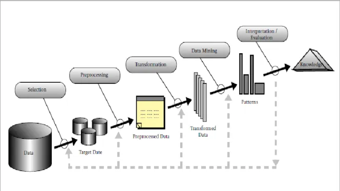
KDD is the nontrivial process of identifying valid, novel, potentially useful, and ultimately understandable patterns in data (Fayyad, Piatetsky-Shapiro, & Smyth, 1996). The aim of the KDD process is to garner insights from large datasets. Figure 2.1 provides an overview of the steps involved in gathering information and knowledge from sources of data (Fayyad et al., 1996). The KDD process consists of several stages, selection, pre-processing, transformation,
10
data mining and interpretation/evaluation. Association rule mining is one data mining application to extract patterns in data.
Figure 2.1: Overview of the KDD Process (Source: Fayad et al., 1996)
Data Mining forms one of the steps in the KDD process. The goal of the data mining step is to identify patterns which can then be interpreted and allow for more informed decisions to be taken. The authors state that “Data mining is a step in the KDD process that consists of applying data analysis and discovery algorithms that, under acceptable computational efficiency limitations, produce a particular enumeration of patterns (or models) over the data”.
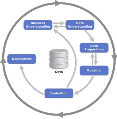
There are several frameworks that outline a process to deliver a successful data mining project summarised in table 2.1. The two most well-known frameworks are CRISP-DM and SEMMA. The Cross Industry Process for Data Mining or CRISP-DM is a commonly used process to complete a data mining project. The CRISP-DM (Shearer, 2000) process presents six phases of the data mining process, business understanding, data understanding, data preparation, modelling, evaluation and deployment. The arrows between different process
11
steps in Figure 2.2 highlight the iterative nature of a data mining project where insights and results from one step can inform previous or future steps in the process.
Figure 2.2: CRISP-DM Data Mining Process Model (Source: Shearer, 2000)
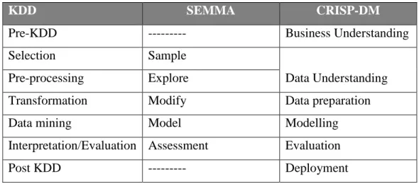
The SEMMA process consisting of sample, explore, modify, model and assess is a list of sequential steps developed by the SAS Institute. It is often noted that the SEMMA process lacks business focus (Azevedo & Santos, 2008) in its process, unlike the CRISP-DM process which includes the business understanding phase as the first phase. Although gathering the domain and problem knowledge is not specifically identified as a phase in SEMMA, it is argued that it is not feasible to start a project without this understanding and therefore it is assumed that this forms part of the sample phase in SEMMA. Azevedo & Santos (2008, p. 5) state “we can integrate the development of an understanding of the application domain, the relevant prior knowledge and the goals of the end-user, on the Sample stage of SEMMA, because the data cannot be sampled unless there exists a true understanding of all the presented aspects”. Table 2.1 below neatly summarises the comparison of the three methodologies discussed above.
12
KDD SEMMA CRISP-DM
Pre-KDD --- Business Understanding
Selection Sample
Data Understanding Pre-processing Explore
Transformation Modify Data preparation
Data mining Model Modelling
Interpretation/Evaluation Assessment Evaluation
Post KDD --- Deployment
Table 2.1: Comparison of KDD, SEMMA and CRISP-DM
Within the Data Mining step of the knowledge discovery process, there are three primary forms of learning algorithms namely supervised, unsupervised and reinforcement learning algorithms.
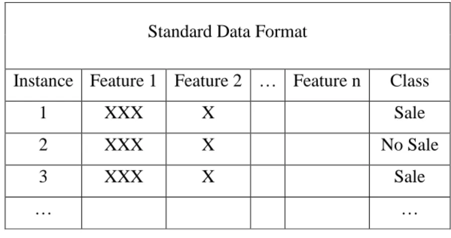
In supervised learning, the data provided to the model has known class labels which are the corresponding correct outcomes. For supervised learning tasks, the data is usually represented in a table similar to Table 2.2. Supervised learning algorithms create a function that models the data using historic data instances and the function is then applied to predict the outcome of previously unseen data. The function created on historic data is used to score new previously unseen data instances. Real-world examples of supervised learning include spam detection (Androutsopoulos, Koutsias, Chandrinos, Paliouras, & Spyropoulos, 2000), default prediction models in financial services (Atiya, 2001), cancer prediction in health services (Shipp, Ross, Tamayo, Weng, Kutok, Aguiar, & Ray, 2002) and voice recognition (Hinton, Deng, Yu, Dahl, Mohamed, Jaitly, & Kingsbury, 2012). The data mining algorithms used to perform supervised learning tasks include logistic regression (McCullagh, 1984), decision trees (Quinlan, 1986), random forests (Breiman, 2001), support vector machines (Cortes & Vapnik, 1995) and neural networks.
13
Standard Data Format
Instance Feature 1 Feature 2 … Feature n Class
1 XXX X Sale
2 XXX X No Sale
3 XXX X Sale
… …
Table 2.2: Sample Dataset for Supervised Learning
Another form of data mining is reinforcement learning (Barto & Sutton, 1997). Reinforcement learning is learning what to do and mapping situations to necessary actions. In reinforcement learning, the learner is not told what to do but instead must learn what action yields the maximum reward. An example of reinforcement learning is teaching an agent how to play computer games such as Super Mario or Pac Man. An example of a reinforcement learning algorithm is Q-learning (Watkins, 1992). In Q-learning, the goal is to reach the state with the highest reward, so that if the learner arrives at the goal, it will remain there indefinitely. In reinforcement learning this type of goal is called an absorbing goal.
Unsupervised learning is applied where data instances are unlabelled. The dataset is typically similar to Table 2.2 above, however, the class label for prediction is not available. By applying these unsupervised algorithms, researchers hope to discover unknown, but useful, classes of items (Jain et al., 1999). Some of the most well researched unsupervised learning algorithms include clustering, anomaly detection and association rule learning.
Considerable research has been carried out on supervised learning techniques to predict classes including models such as decision trees and neural network approaches. More recent studies (Liu et al., 1998; Li et al., 2001) propose the use of unsupervised association rules for classification purposes by using a set of high-quality association rules to make the class predictions.
14
2.3 Association Rule Learning
Association rule learning, a form of dependency modelling3, examines the dataset for relationships between variables or items. The classical application of Association Rule algorithms is within the context of retail store shopping transactions and the items within those transactions (Agrawal et al., 1993). The analysis of association rules in retail store databases is more commonly known as Market Basket Analysis. The general concept of association rule learning is to identify rules such as a customer who buys product A also buys product B with an identifiable confidence level. Another area where association rules have been employed is in medical research to identify high-risk patients (Obenshain, 2004) and the early identification of infection (Brossette, Sprague, Hardin, Waites, Jones, & Moser, 1998).
When applying association rule algorithms, the objective is completeness, the algorithm is required to find all interesting rules in the dataset. The difficulty with association rule mining is the size and complexity of the problem. The number of possible rules in the dataset increases exponentially with the number of items. The algorithms developed for association rule mining attempt to reduce this level of complexity and provide fast results from the models developed.
The idea of applying Association Rule Mining to Market Basket Analysis was introduced by (Agrawal et al., 1993). Formally, the problem of association rule mining is defined as: Let 𝐼 = {𝑖1, 𝑖2, … 𝑖𝑛} be a set of n distinct literals called items. Let 𝐷 = {𝑡1, 𝑡2, … 𝑡𝑚} be a set of transactions in the database. Each transaction T is unique and contains a number of items from I.
An association rule is a conditional implication among itemsets, 𝑋 => 𝑌 where X, Y are items. In order to identify interesting rules in the dataset, there are two key metrics in measuring association rule mining results, the support and the confidence of the rule.
The support supp(X) is defined as the proportion of transactions in the dataset which contain the itemset X and reflects its statistical significance. In simple terms, the number of transactions which contain X in the transaction is divided by the total number of transactions.
15
The confidence of any rules identified is measured as the percentage of transactions containing Y which also contain X, divided by the number of transactions which contain X within the whole dataset. This identifies how often the identified combination occurs together. Confidence is the measure to monitor the individual strength of the association rules identified.
The goal of association rule mining is to find all association rules which exceed some user-defined minimum levels for both support and confidence.
To identify the association rules within a dataset using an association rule algorithm there are typically two steps.
1. The first step is to identify all combinations of itemsets that meet the user identified minimum support (minsupp) thresholds set. These itemsets are said to be large or frequent itemsets and those that do not meet the support level are said to be small or infrequent itemsets.
2. The second step is to measure the confidence of each rule and compare against the minimum confidence level chosen (minconf).
Once the rules that meet the minimum support threshold are identified the second step is rather straightforward (Agrawal et al., 1993). The algorithms for association rule learning focus predominately on the first sub-problem above and try to reduce the computationally expensive task of identifying all rules which are above the user-defined support level.
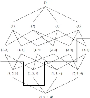
As the number of items increases, there is an exponentially growing number of itemsets which need to be assessed. For example, if |I| = m, the number of possible distinct itemsets is 2𝑚, which forms a lattice of subsets over I. Typically, only a very small number of the itemsets in this exponentially large subset will meet the minimum support levels set. Figure 2.3 (Hipp, Güntzer, & Nakhaeizadeh, 2000) provides an illustration of the itemsets that need to be assessed with 4 items.
16
Figure 2.3: Lattice for I = {1,2,3,4} (Source: Hipp et al., 2000)
The main problem in association rule mining is identifying itemsets which meet the user- defined minimum support level. When using these algorithms in practice with a large number of items, assessing each itemset is not possible as the size of the search space is too large.
To reduce the size of the search space the algorithms rely on the downward closure property (Agrawal & Srikant, 1994) which prevents the algorithm from counting itemsets which will not be frequent at the end. Employing this property significantly reduces the number of itemsets to be assessed.
There are four main types of association rule algorithms, each of which employs a different strategy for identifying itemsets that meet the minimum support level defined. The variances between the models are whether the algorithm employs breath first search or depth-first search and secondly whether the algorithm uses candidate generation or set intersecting to determine the support values of candidates. Within set intersections the algorithms use a tidlist. A TID is a unique transaction identifier for all transactions in the databases. For each item in I the relevant tidlist is a list of all transaction ids for transactions which contain the item. The use of tidlists is applied in the Partition and EClat algorithms.
17 2.3.1 AIS Algorithm
In Agrawal et al. (1993), the authors first introduced the idea of mining large datasets for association rules. The authors presented the AIS algorithm which generated new itemsets by extending out large itemsets found in the previous database pass with other items in the transactions, a step known as candidate generation. This resulted in a large number of itemsets being counted which would ultimately turn out not to meet the minimum support levels set. Houtsma and Swami (1995) subsequently presented an algorithm called SETM which introduced the idea of trying to solve the association rule problem using a relational database.
2.3.2 Apriori Algorithm
Agrawal et al. (1994), presented the Apriori and AprioriTID algorithms. The Apriori Algorithm uses a breath-first search and builds on previous algorithms through the application of the downward closure property to reduce the number of itemsets which need to be counted and therefore run more efficiently. In the paper the authors present the following lemma, “The basic institution is that any subset of a largest itemset must be large. Therefore, the candidate itemsets having k items can be generated by joining large itemsets having k – 1 items, and deleting those that contain any subset that is not large. This procedure results in the generation of a much smaller number of candidate itemsets” (Agrawal et al., 1994, p.4).
For example, if it is found the itemset {1,2,3} is small, then none of the itemsets which are extensions of {1,2,3} such as {1,2,3,4} or {1,2,3,5,7} need to be tested for minimum support. In practice, the Apriori algorithm prunes particular sets as it makes passes over the database and does not count any itemset in the next pass where a subset of the itemset did not meet the support level required in a previous pass. One of the criticisms of the Apriori algorithm is that the algorithm requires multiple passes over the database which can be computationally expensive.
The AprioriTid (Agrawal et al., 1994) aims to address the computationally expensive nature of the Apriori algorithm. AprioriTid encodes all the large itemsets in a transaction after the first pass to prevent having to pass over the database itself in subsequent passes. In subsequent passes, the level of transactions can be much smaller than the database, however,
18
for initial passes, the encoding of the transactions may be larger than the actual database. To overcome this issue, the authors propose a hybrid of Apriori and AprioriTid named Apriori Hybrid, which uses Apriori for earlier passes and AprioriTid for later passes.
The authors compared the performance of the two new algorithms with the previous algorithms AIS and SETM. The results showed that the performance gap, in favour of the two new algorithms, increased as the size of the problem increased, ranging from a factor of three for small problems to more than an order of magnitude for large problems.
The CBA algorithm for performing classification using association rules extends the Apriori algorithm to make class predictions.
2.3.3 Partition Algorithm
Savasere, Omiecinski, and Navathe (1995) present an alternative method for association rule mining known as the partition algorithm. The objective of the partition algorithm is to reduce the number of required passes over the database to identify large itemsets. Reducing the number of passes the algorithm needs to make over the database reduces the run time and reduces the impact on the underlying hardware system (Savasere et al., 1995).
The partition algorithm requires only two passes over the database. In the first pass of the database, the algorithm splits the database into a number of non-overlapping smaller partitions and then identifies all large itemsets within each of the smaller sets. The model ensures that the partition sizes are chosen to ensure there are no difficulties in relation to the main memory. In the second pass, these large itemsets are joined together, their actual count and support is calculated and those that meet the target support level are identified. The second step ensures that the itemsets which are found to be large in each partition i.e. locally supported are also supported globally on the full database.
Similar to the Apriori Algorithm the Partition Algorithm employs the downward closure property and prunes itemsets which are found not to be large from being considered for counting support.
19
In testing the model against previous algorithms, the authors used the same synthetic data as in Agrawal et al. (1994). The author’s tests showed that the Partition Model outperformed the Apriori model by up to a factor of seven while also reducing the levels of CPU usage and I/O.
2.3.4 Frequent Pattern (FP) Growth Algorithm
Han, Pei, and Yin (2000) developed a new approach to identifying association rules moving away from an Apriori-like approach. Apriori algorithms use a generate and test approach which involves generating itemsets and then testing if they are frequent. Identifying frequent itemsets is the costliest element of Apriori-like algorithms. The authors note that applying the downward closure property (Agrawal et al., 1994) achieves good performance gain on previous algorithms but is still very costly in terms of performance in situations where there are a large number of frequent itemsets or the minimum support thresholds are low.
The FP Growth model proposes an alternative approach to identifying frequent itemsets which does not rely on candidate generation. The FP Growth model works in two steps:
1. The model converts the transactions in the database into a more compact data structure, a Frequent Pattern Tree (FP Tree) which is built using two passes of the database.
2. In the second step, the model then uses the FP tree constructed rather than the database to find frequent patterns.
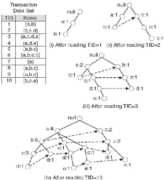
The FP Tree is constructed using two passes over the database; in the first pass the support for each item in the database is calculated and infrequent items are pruned. Frequent items are sorted in a fixed order to ensure efficiency. Then in the second pass the FP tree is constructed and all transactions are mapped to a path on the tree and the counting is completed. As certain transactions may have items in common their paths may overlap, this is taken into account when building the FP Tree and therefore reduces the size of the data structure. Figure 2.4 (Tan, 2006) below outlines the process of creating an FP-tree for 10 transactions (TIDs). Where subsequent transactions follow similar paths the nodes of the tree will increase the count by 1.
20
Figure 2.4: FP Tree for 10 Transactions Dataset (Source: Tan, P. N., 2006)
Once the tree is created to identify frequent patterns “the search technique employed in mining is a partitioning-based, divide and conquer method rather than an Apriori-like bottom up generation of frequent itemset combinations” (Han et al., 2000, p.2).
In order to identify the frequent patterns, the authors create prefix path sub-trees for each item set. Each prefix path sub-tree is then processed recursively to extract the frequent itemsets. Based on the prefix path the model creates conditional FP Trees for each itemset.
The authors test the FP growth model against the candidate generation models and find that the model is about an order of magnitude faster than Apriori.
The CMAR algorithm for classification using association rules is an extension of the FP-growth algorithm for association rule learning.
21 2.3.5 Equivalent Class Transformation Algorithm
Zaki, Parthasarathy, Ogihara and Li (1997) present four new algorithms which only require one pass over the database. The algorithms presented by the authors differ to Apriori-like algorithms in that they traverse the prefix tree in depth-first order compared to breath-first search in the Apriori algorithm. The most important algorithm presented, EClat, relies on tid-lists as described above. Each transaction has a transaction id or tid, a tid-list is a list of all the transactions which contain a particular item. The Eclat model determines the support of any k-itemset by intersecting tid-lists of two of its (K-1) subsets. The authors state this as ‘We partition Lk into equivalence classes based on their common K-1 length prefix, given as [a] = [b[k]|a[1:k-1] = b[1:k-1]}’.
The authors propose that a vertical format for storing the transactional data is more applicable to association rule mining than a horizontal format. Under this method, the model only needs to make one pass of the database. Both Apriori and FP Growth use horizontal data format which starts with the transaction id and the itemsets within the transaction. The vertical format starts with the itemset and lists all transactions which contain that itemset. The authors state that a “vertical format seems more appropriate for association mining since the support of a candidate k-itemset can be computed by simple tid-list intersections” (Zaki et al., 1997, p.285). Figure 2.5 shows an example of a tid-list intersection.
Figure 2.5: Example of tid-list intersection
The authors compare the new algorithms presented against Apriori and Partition (with 10 partitions). The authors state that EClat outperforms Apriori by a factor of 10 and Partition by a factor of 5. The authors also state the new models scale well as the transactions sizes
22
increase. The advantage of this algorithm is that the depth-first search can result in much faster results, however, the intermediate tid-lists may become too large for memory.
2.3.6 Conclusion Association Rule Learning Algorithms
Zheng, Kohavi and Mason (2001) performed the first evaluation and comparison of association rule learning algorithms on real-world datasets. In this experiment, the authors evaluated five of the state of the art association rule algorithms including Apriori and FP-growth. The authors evaluated performance on three real-world datasets and one artificial dataset using a range of minimum support values to test performance and scalability. For the artificial dataset, every algorithm outperformed Apriori by a significant margin for minimum support values less than 0.10%. FP-growth was one order of magnitude faster than Apriori when the minimum support was set to 0.02%. This evidence is consistent with the results of other previous experiments (Han & Pei, 2000; Zaki, 2000). The performance improvement of FPgrowth over Apriori increases as the minimum support decreases, indicating that FP-growth scales better than Apriori. For all of the real-world datasets, FP-FP-growth is faster than Apriori, but the differences are not as large as on the artificial dataset. The reasoning proposed by Zheng et al. (2001) is that the artificial dataset has different characteristics to the real world datasets.
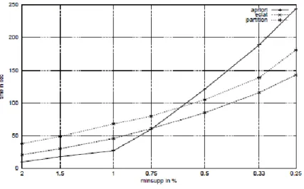
In Hipp et al. (2000), the authors compare a number of association rule algorithms on efficiency by carrying out several runtime experiments on synthetic data. The authors compare Apriori, DIC a variation of Apriori (Brin, Motwani, Ullman, & Tsur, 1997). Partition and Eclat. The authors state that the results of the experiments indicate that the runtime behaviour of the various algorithms is more similar than expected. Only in certain more extreme cases did the authors evidence varying performance. In Figure 2.6 one of the experiments on a more complex dataset shows Eclat and Partition performing better than Apriori, particularly at low minimum support levels.
23
Figure 2.6: Comparison of association rule algorithms across varying support levels (Source: Hipp et al., 2000)
Heaton (2016), compared the performance of Apriori, Eclat and FP-growth across varying artificially created datasets. Two dataset characteristics were evaluated, maximum transaction size and frequent item density and the algorithms were tested under various conditions. The results demonstrate that Eclat and FP-Growth both handle increases in maximum transaction size and frequent itemset density considerably better than the Apriori algorithm, while FP-growth marginally outperformed Eclat. Figure 2.7 below shows the results of the tests for various frequent itemset densities. It shows that all three of the algorithms perform to a similar level up to roughly 70% at which point the performance of Apriori considerably deteriorates.
Figure 2.7: Comparison of association rule algorithms across varying itemset densities (Source: Heaton, 2016)
24
2.4 Extending Association Rules to make predictions
In data mining, making class predictions is typically associated with supervised learning. Supervised learning aims to create a function or set of rules to accurately classify labels and then the rules or function are applied to newly unseen data to make predictions. Association rule mining is an unsupervised learning approach that finds all rules in the database that satisfy some minimum support and minimum confidence constraints, for example Agrawal and Srikant (1994). Liu et al. (1998) propose a framework to combine these two techniques of data mining. The authors propose an integrated framework, called associative classification. The framework concentrates on a subset of association rules where the right-hand side of the rule is restricted to the class being predicted. This subset of rules is called class association rules.
The approach to associative classification involves three key steps:
Association Rule Learning – Adaptation of association rule
learning algorithms to generate the CARs
Application of a rule pruning technique
Use Rules to make Classifications - Building a classifier from the generated
rules
2 1
25 2.4.1 Generating Interesting Rules
Liu et al. (1998) propose a new algorithm CBA with two parts, a rule generator CBA-RG and CBA-CB which uses the rules generated to build classifications. To use association rules for classification the underlying algorithms described in Section 2.3 above need to be adapted. The CBA-RG is an adaptation of the Apriori algorithm described in Section 2.3. Class association rules are a subset of all association rules where the right-hand-side is restricted to a distinct class label. Class association rules or itemsets take the form <condset,y> where y is a class label. The CBA-RG identifies frequent itemsets with high support and high confidence within the subset of rules.
Support is defined as 𝑟𝑢𝑙𝑒𝑠𝑢𝑝𝐶𝑜𝑢𝑛𝑡
|𝐷| where rulesupCount is the total count of a particular itemset and D is the total database. Itemsets that satisfy a set minimum support level are deemed frequent and other remaining itemsets are deemed infrequent.
The confidence of the itemset is defined as 𝑟𝑢𝑙𝑒𝑠𝑢𝑝𝐶𝑜𝑢𝑛𝑡
𝐶𝑜𝑛𝑑𝑠𝑢𝑝𝐶𝑜𝑢𝑛𝑡 where CondsupCount is the total count of the condset within D.
For example, if there is a rule {Age: 25-35, Location: Dublin} -> Sale. If the count of the condset {Age: 25-35, Location: Dublin} is 3 and the count of the itemset {Age: 25-35, Location: Dublin} -> Sale is 2 and the total database is 10. The support of the itemset is 2 / 10 or 20% and the confidence of the itemset is 2/3 or 66.67%.
The CBA-RG outputs all CARs that meet the minimum support and minimum confidence levels. For itemsets with the same condset the algorithm chooses the itemset with the highest confidence. The criticism of CBA-RG is that the algorithm outputs only a single high-confidence rule. This may lead to biased classifications that overfit the data. Verhein and Chawla (2007) challenge the ability of CBA to build an accurate classifier on imbalanced datasets.
Li et al. (2001) propose a new algorithm Classification Based on Multiple Association Rules (CMAR) to overcome the restrictions inherent in CBA. The authors propose the use of more rules to support the class prediction problem. The requirement to store many more rules,
26
however, has an impact on the combinatorial explosive nature of association rules as described in Section 2.3. If |I| = m, the number of possible distinct itemsets is 2𝑚. In CMAR, the authors propose the use of multiple high-quality rules to make a classification decision rather than restricting the decision to the rule with the highest confidence score as applied in the CBA algorithm.
For example, suppose there is a new database instance {Age: 25-35, Location: Dublin, Job: Accountant} and the Bank wants to determine whether this customer is likely to take out a mortgage for home purchase. The three rules with the highest confidence for this customer are as follows:
• Rule 1, {Location: Dublin} -> No Sale (Support 20%, Confidence 90%)
• Rule 2, {Age: 25-35} -> Sale (Support 30%, Confidence 87%)
• Rule 3, {Job: Accountant} -> Sale (Support 25%, Confidence 85%)
Using the CBA algorithm Rule 1 would be chosen for classification purposes given it is the rule with the highest confidence, however, the other two rules both have higher support and only marginally lower confidence. The objective of CMAR (Li et al., 2001) is to use a number of high-quality rules to make a more balanced decision to classification and increase prediction accuracy over CBA by reducing the levels of overfitting.
To find rules for classification, CMAR adopts a variant of the FP-growth method explained in Section 2.3. The FP-growth model is faster than the Apriori model particularly in situations where there are a large number of frequent itemsets or the minimum support thresholds are low (Hipp et al., 2000). One of the major advantages of the CMAR adaptation of FP-growth is that it is capable of identifying frequent itemsets and generating rules in one pass while traditional algorithms like Apriori and Apriori extensions such as CBA require two passes. In Apriori, first all items that pass the minimum support levels are identified and then in the second step, the confidence of frequent itemsets are calculated. In the CMAR algorithm, however, “CMAR maintains the distribution of various class labels among data objects matching the pattern. This is done without any overhead in the procedure of counting (conditional) databases. Thus, once a frequent pattern (i.e., pattern passing support
27
threshold) is found, rules about the pattern can be generated immediately” (Li et al., 2001, p. 4). This is a major advantage for CMAR over CBA in the rule generation phase.
2.4.2 Data Storage CR-tree representation
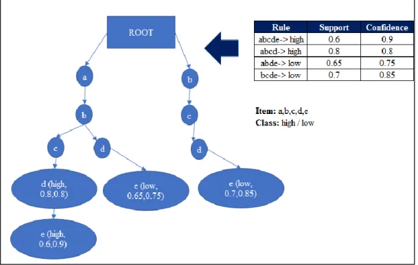
Li et al. (2001) also propose a new approach to data storage and retrieval of a large number of association rules. The authors present a structure called a CR-tree which is a prefix tree structure. CR tree is a prefix tree structure that exploits sharing among rules. The main advantage of the CR-tree structure is that the representation of the data in this way means rules can be stored in a compressed way thus saving memory. The authors state that in their experiments about 50-60% of space can be saved by using a CR-tree structure to store the data.
Figure 2.8 below shows an example of the compression capability of CR-tree. A CR-tree has a root node. All of the values from the left-hand side of the association rules are sorted according to their frequency. The first rule abcd -> high is inserted in the tree, the class and the support and confidence of the rule are stored at the node. The next rule abcde -> high is then inserted but is simply an extension of the last rule where e is added as a new node, again the class, support and confidence are registered with the node. Storing each element of the left-hand side of the rules individually would require 17 cells while in this CR-tree representation just 11 cells are needed so a saving of 35% in this example.
2.4.3 Pruning
The number of rules generated from the Association Rule mining stage can be extremely large. In order to reduce the quantity of rules to a smaller number that are effective and efficient for classification purposes, a post pruning strategy is required. There are a number of pruning approaches employed across the state of the art models for classification using association rules. Across, the CBA and CMAR algorithms there are both similarities and differences to the pruning strategies employed.
28
Figure 2.8: Example of the compression capability of CR-tree
Both the CBA and CMAR algorithm generate a global order of rules or a rule precedence. Given two rules R1 and R2, R1 ranks above R2 as follows:
(1) Confidence R1 > Confidence R2
(2) Confidence R1 = Confidence R2 but Support R1 > Support R2
(3) Confidence R1 = Confidence R2 and Support R1 = Support R2 but R1 has fewer attributes on the left-hand side than R2.
The CMAR algorithm implements three steps in the pruning process. First, CMAR employs general to specific ordering. A rule R1 is said to be a general rule w.r.t R2, if the left-hand side of R2 is a subset of the left-hand side of R1. CMAR uses general and high-confidence rules to prune more specific and lower confidence rules. Given two rules, R1 and R2, where R1 is a general rule w.r.t R2. CMAR prunes R2 if R1 also has a higher rank than R2. More general rules are favourable to reduce overfitting and improve the ability for the model to generalize.
In the second pruning step, CMAR uses a statistical measure to further prune the rule set. In this step, CMAR selects only positively correlated rules. For each rule, R: P -> C, the
29
algorithm tests whether P is positively correlated with C using 𝑥2 testing. Only rules that are positively correlated and above a certain statistical significance threshold are carried forward for use in classification. To perform the chi-square test, the rule R is tested against the whole database.
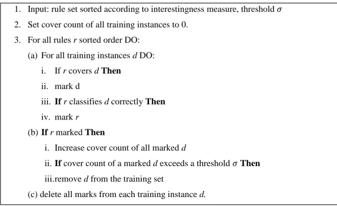
In the third pruning step, CMAR uses database coverage to prune rules. Database coverage ensures that each rule brought forward to the classification model can classify at least one training instance correctly. Database coverage also ranks the rules by precedence ensuring that the rules brought forward are those rules with the highest ranking among rules that can cover the instance. In association rule learning, a rule R covers an instance d if the attributes of the instance satisfy the condition of the rule. An example of rule coverage is outlined below using two example rules.
R1 (Age 45 – 55 = Yes), (Employed = No) -> No Sale R2 (Age 25 – 35 = Yes), (Occupation = Mechanic) -> Sale
Name Age Employed Occupation Location Class
Colin 25 - 35 Y Mechanic Dublin Sale
John 45 - 55 N Unemployed Galway No Sale
R1 covers the instance John R2 covers the instance Colin
In this pruning step, CMAR retains more rules than CBA. In the CBA algorithm, once one rule covers an instance the instance is removed from the training dataset. In CMAR, in order for an instance to be removed, the instance must be covered by some threshold number of rules 𝛿 (in CBA 𝛿 = 1). Once the threshold is achieved all of these rules are brought forward for classification. The pruning approach is outlined in Figure 2.9. The CMAR approach increases the number of rules brought forward for classification purposes but should lead to less overfitting as a number of rules are used to make a collective decision when a new instance is to be classified. Li et al. (2001) state that their approach CMAR, using multiple rules for prediction, leads to higher average class accuracy than CBA and C4.5.
30
Figure 2.9: Pruning using database coverage.
(Source: The scheme is an adapted version from Li et al. (2001) and Liu et al. (1998))
As described above, CBA uses a simpler version of database coverage than CMAR for pruning where the threshold 𝛿 is set to one. This results in a smaller set of rules brought forward to be employed in the classification model. CBA also employs a number of additional obligatory and optional pruning steps. The additional obligatory pruning step completed in CBA is called default rate pruning and the optional pruning step is pruning based on the pessimistic error rate (Quinlan, 1993).
The CBA algorithm uses three steps to perform the default rate pruning process. Using the rule precedence set out above the rules are sorted based on highest precedence. Rules with the highest confidence are ranked at the top. Figure 2.10 below outlines the method applied where R is the set of sorted rules. Lines 2 – 12 below, select rules from R. For each rule r, go through D to find those cases covered by r (line 5). R is then marked if it correctly classifies a case d. d.id is the unique identification number of d. If r can correctly classify at least one case, it will be a potential rule for use in the classification stage. Those cases it covers are then removed from D (line 9). A default class is also selected (the majority class in the remaining data), which means if the algorithm stopped selecting more rules to include in the
1. Input: rule set sorted according to interestingness measure, threshold 𝜎
2. Set cover count of all training instances to 0. 3. For all rules r sorted order DO:
(a) For all training instances d DO: i. If r covers d Then
ii. mark d
iii. If r classifies d correctly Then
iv. mark r
(b) If r marked Then
i. Increase cover count of all marked d
ii. If cover count of a marked d exceeds a threshold 𝜎Then
iii.remove d from the training set