Wavelet Analysis of Transonic Buffet
on A Two-dimensional Airfoil
with Vortex Generators
Toshinori Kouchi (Corresponding author)
Dept. Mechanical and System Engr., Okayama University
Tsushimanaka 3-1-1, Kita, Okyama, Okayama 700-8530, Japan
Tell: +81-86-251-8045 / Fax: +81-86-251-8045 E-mail: [email protected]
Shingo Yamaguchi
Dept. Mechanical and System Engr., Okayama University
Tsushimanaka 3-1-1, Kita, Okyama, Okayama 700-8530, Japan
Shunske Koike
Next Generation Aeronautical Innovation Hub Center, Aeronautical Technology
Directorate, JAXA
Jindaiji higashi 7-44-1, Chofu, Tokyo 182-8522, Japan
Tsutomu Nakajima
Aerodynamics Research Unit, Aeronautical Technology Directorate, JAXA
Jindaiji higashi 7-44-1, Chofu, Tokyo 182-8522, Japan
Mamoru Sato
Aerodynamics Research Unit, Aeronautical Technology Directorate, JAXA
Jindaiji higashi 7-44-1, Chofu, Tokyo 182-8522, Japan
Hiroshi Kanda
Aerodynamics Research Unit, Aeronautical Technology Directorate, JAXA
Jindaiji higashi 7-44-1, Chofu, Tokyo 182-8522, Japan
Shinichiro Yanase
Dept. Mechanical and System Engr., Okayama University
Tsushimanaka 3-1-1, Kita, Okyama, Okayama 700-8530, Japan
Abstract
We visualized the shock-buffets on a two-dimensional transonic airfoil with and without vortex generators (VGs) by using a fast-framing focusing schlieren imaging. The focus-ing-schlieren visualization showed that the flow three-dimensionality around the airfoil became remarkable with installing the VGs. This implies that narrow depth of focus of imaging systems was key to accurately capture the characteristics of the shock oscillation due to the buffet for the cases with VGs. The time-resolved imaging also revealed that non-periodic components were included in the shock-oscillation due to the buffet for the cases with VGs. This prevented Fourier analysis from being applied. We used wavelet analysis to extract the characteristic of the shock oscillation for the cases with VGs. The wavelet spectrograms revealed that the low frequency oscillation having the buffet frequency was still included intermittently in the shock oscillation even when VG controlled the buffet. The rate of appearing the low frequency oscillation increased with increasing both the interval between VGs and the angle of attack.List of Symbols
AoA = angle of attack, °c = chord, mm
DOF = depth of focus, mm
DVG = interval between vortex generators, mm
f = frequency in a Fourier domain, Hz
f’ = frequency in a wavelet domain, Hz
fB = dominated frequency of shock-buffet (buffet frequency), Hz
HVG = height of a vortex generator, mm
M = Mach number
PSD = power spectrum density function of shock oscillation, mm2/Hz
P0 = stagnation pressure of freestream, Pa
Re = Reynolds number
t = time, s
T0 = stagnation temperature of freestream, K
VGs = vortex generators
1
Introduction
Shock-wave boundary-layer interaction (SWBLI) on an airfoil induces a massive flow separa-tion and leads to large-scale self-induced shock oscillasepara-tion in a transonic flow, when flight Mach number of the aircraft and/or its angle of attack (AoA) increase. This instability is known as buffet
and can lead to structural vibrations (buffeting). The buffeting greatly affects the aerodynamic behavior of the aircrafts and limits their flight envelope. Therefore, the research community has been conducting the experiments and simulations on the buffet, to understand the physics of the buffet, to predict the onset of the buffet and to explore the buffet control techniques.
Lee (2001) performed one of the very detail investigations of two-dimensional transonic buffet. He proposed the self-sustained mechanism of the shock oscillation due to the buffet. In his model, the pressure disturbance is generated at the shock foot on the airfoil and propagated downstream within the boundary layer. This pressure disturbance directly feeds back as upstream traveling pressure waves (sometimes called as Kutta waves) generated at the trailing edge of the airfoil. The round trip time of the pressure waves determines frequency of shock oscillation due to the buffet (buffet frequency). This model fairly reproduced the experimental data (Lee 2001, Jacquin et al. 2009, and Zhao et al. 2013).
Other different paths for the pressure waves were also proposed to sustain the shock oscillation (Stanewsky & Baster 1990, Crouch et al. 2007). Stanewsky and Basler (1990) mentioned that the upstream propagating Kutta waves on the lower surface of the airfoils play an important role to sustain the shock oscillation. Jacquin et al. (2009) measured the fluctuating pressure on OAT15A airfoil and experimentally confirmed the existence of the Kutta waves traveling on the lower sur-face of the airfoil. They also showed that the estimated buffet frequency using the time scale of the lower surface Kutta waves better agreed with the experimental data, compared with those using the upper one. In addition, Crouch et al. (2009) observed another path of the pressure disturbance in their simulation. The pressure disturbance propagated along the shock wave in the height-wise direction and tuned to the leading edge of the airfoil through the outside the supersonic region. His observation was qualitatively different from the model proposed by Lee (2001). Thus, the buffet mechanism has not been fully understood yet.
Many research groups have been developing the devices to control the buffet and investigating the flow physics related to them. The buffet control devices are mainly categorized into two types:
active and passive devices. Boundary layer bleeding and injection of different gas are traditional methods to control the boundary layer separation (Schlichting 1979). Molton et al. (2013) tested supersonic air injections on the swept wing model as the active buffet control device and compared them with mechanical vortex generators (VGs). Vortex generator is one of the most popular and traditional passive devices to control the buffet. Titchener and Babinsky (2015)reviewed the re-searches on the vortex generators. The installation of VGs induces streamwise vortices and in-creases momentum transfer into boundary layer. In addition, the installation of VGs partitions the separation region into number of the cells. These mitigate shock-induced separation and delay the buffet. However, the installation of VGs drawbacks to increase the drag in a nominal cruise condi-tion (Kusunose & Yu 2003). Therefore, we have to optimize the configurations of the VGs, for example, number and height of the VG, interval between the VGs and etc.
The optimal values for the configurations on the airfoil are usually found and confirmed by the parametric experiments (Koike et al. 2013 & 2015), simulations (Ito et al. 2016) and multi-objective optimizations using CFD (Kozakai et al. 2015, Namura et al. 2016). These values are still difficult to predict empirically by using a conceptual model of the VG. We believe that both understanding of the physics on the buffet and development of the conceptual model of VG on the airfoil requires the detail time-resolved spatial information on the buffet for the cases with and without VGs, such as shock motion and pressure waves propagation which play an important role to sustain the shock oscillation (Lee 1990). To obtain this information, we developed a fast-framing focusing schlieren imaging system to capture the shock oscillation and the pressure wave propagation in the flowfield around the airfoil and capture the buffet for the cases without VGs (Yamaguchi et al. 2015). In this study, we applied this imaging system to the experiments of two-dimensional transonic buffet with VGs and investigated the characteristics of the shock motion.
In the cases without VGs, the previous works reported that the shock-buffet was quit periodic. Therefore, Fourier analysis could easily extract the characteristics of the shock motion. However, we found that the shock wave oscillation were not periodic with installing VGs. Therefore, we applied the wavelet analysis, instead of the Fourier analysis, to extract the characteristics of the shock motion and report them in this work.
2
Wind Tunnel Experiments
2.1
Two-dimensional Airfoil
The experiments were conducted in a two-dimensional transonic wind tunnel facility of JAXA (NAL Second Aerodynamics Division 1982; NAL Two-dimensional Transonic Wind Tunnel Laboratory 1999). The wind tunnel was a blow-down type facility and supplied a high-pressure compressed air to achieve high Reynolds number (Re) conditions. The test section had a 0.8 m x 0.45 m cross-section and sited in a plenum chamber. The top and bottom walls of the test section had slots to realized transonic flow conditions for a relatively large wing model. Stagnation pres-sure (P0) and temperature (T0) were 200 kPa and 300 K, respectively. The nominal freestream Mach before the wall interference correction (Sawada 1978)was 0.7. These conditions realized the nominal Re based on the chord length (c) of 5 millions.
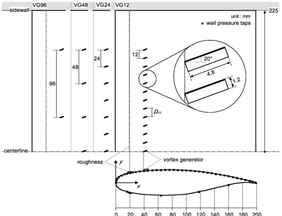
Figure 1 shows a two-dimensional supercritical airfoil of NASA SC(2)-0518 (Harris 1990) used in this study. Cartesian coordinate system was used to represent the experimental results, with the origin at the center of the leading edge of the airfoil, the chord direction on the x-axis, height from the chord on the y-axis and the spanwise direction of the airfoil on the z-axis. The airfoil was supported between two sidewall windows of the test section. To reduce the influence of the sidewalls, the boundary layers were bled from the upstream of the window glasses. Oil-flow and steady pressure measurements revealed that no effects of corner separation was ± 150 mm from the center plane of the airfoil at low AoA conditions for our wind tunnel facility with the boundary-layer bleeding (Sato et al. 2010 and Koike et al. 2013). The sweptback angle of the model was zero. The chord and span lengths of the airfoil were 200 mm and 450 mm, respectively. The model AoA was set from 4° to 7° for each test run. These set AoA are higher by about 1° than the effective AoA obtained by the wall interference correction (Koike et al. 2015). Disk roughness were aligned normal to the freestream with an interval of 0.1 inch both on the upper and lower surfaces of the model at x/c = 0.1. Its diameter and height were 0.05 inch and 0.0031 inch, respec-tively. Attachment of the disk roughness prompted the boundary layer transition (Braslow 1958). Co-rotating rectangular vane-type VGs were installed at x/c = 0.2 on the upper surface of the model. The VGs were aligned with an angle of 20° to the freestream. The length of VGs was 4.8 mm. The height of VGs (HVG) was 1.2 mm. This corresponded to 1.5-times higher than the bound-ary layer thickness at x/c = 0.2. The interval between VGs (D ) was varied from 12 mm to 96
mm for each test run. Five different DVG conditions including without VGs (DVG = ∞) were tested. Note that the VGs were not installed near the sidewalls (|z/c| > 0.75) as shown in Fig. 1.
2.2
Focusing-schlieren Visualization
Schlieren imaging is one of the most popular and relatively straightforward flow visualization techniques for compressible flows. Setup of schlieren is easier than that of other optical measure-ments, for example PIV and PLIF etc, because there are no complications due to leaser sheet optics and tracer seeding equipment. The schlieren imaging, however, has a high sensitivity for capturing not only shock waves but also pressure waves which play an important role to sustain the shock oscillation. In addition, the schlieren imaging is applicable for fast-framing visualization because the technique directly focuses light from the source on an imaging sensor, while many other tech-niques have to collect weak illumination from particles or molecules. Therefore, the technique is
suitable for the studies on unsteady buffet characteristics.
One of the big issues for the schlieren imaging to apply buffet experiments is flow three-dimensionality including the corner separation. Flow three-three-dimensionality blur the motion of shock and pressure waves. This prevents conventional schlieren from being applied to detail
analy-Fig. 1 Two-dimensional supercritical airfoil (NASA SC(2)-0518) and the installation of vortex generators.
sis of unsteady buffet characteristics, because conventional schlieren technique is essentially sensi-tive to the entire length of the light path. Therefore, we applied focusing-schlieren visualization for
this study. The focusing-schlieren has ability to achieve a narrow depth of focus (DOF) compared to the conventional schlieren imaging. Therefore, the technique could reduce capturing unwanted three-dimensional flow structures including the corner separation.
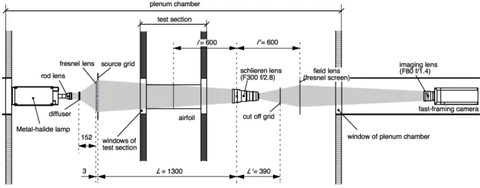
Weinstein’s modern focusing-schlieren system (Settles 2006; Weinstein 2010; Kouchi et al. 2015) was used in this study. Figure 2 shows the schematic layout of the focusing schlieren system for this experiment (Yamaguchi et al. 2015). The system consisted of illuminator and analyzer assemblies. The illuminator consisted of a lamp, light diffuser, Fresnel lens and source grid. This assembly was sited in the plenum chamber. A metal-halide lamp was used as a light source. The continuous light from the metal-halide lamp was diffused by back-projection film and illuminated a source grid that consisted of multiple alternating dark bands and clear apertures to make a two-dimensional light source array. The dark bands were spaced at the same distance as the clear aper-tures of 2 mm. The source grid was photographically made and was placed to emphasize density gradients in the chord direction. The Fresnel lens in front of the source grid condensed the extend-ed light source to increase the light-collection efficiency.
The analyzer consisted of a commercial 35-mm camera lens (schlieren lens), cutoff grid, Fresnel screen and CMOS camera with an imaging lens. The DOF is proportional to distance from the schlieren lens to object (l). The small DOF requires short l. Therefore, the analyzer assembly except for the CMOS camera was also sited on the plenum chamber to minimize DOF. The schlieren lens (300-mm focal length and 2.8 f-number) was placed at 600 mm from the center
plane of the airfoil (z = 0). This setup made the Weinstein’s unsharp DOF ±11.2 mm. This was experimentally confirmed using a 1-mm-diameter, under-expanded supersonic air jet (Yamaguchi et al. 2015).
Flow over an aerofoil after establishing the buffet is three dimensional even for the two-dimensional wing experiments. This is due to the nature of the flow, not just the corner effect in the wind tunnel. Sugioka et al. (2016) measured the unsteady surface pressure on a two-dimensional airfoil of NASA CRM by using Pressure Sensitive Paint (PSP) for similar experimen-tal configuration to our experiments. Their measurements revealed that the averaged and rms pres-sure distributions before and after establishing the buffet were quasi two-dimensional at |z| < 50 mm. The present DOF was smaller than this value. Therefore, we conclude that the present system had enough narrow DOF to reduce capturing the unwanted three-dimensional flow structures in-cluding the corner separation. Details on the effects of DOF are discussed in Sect. 4.1.
The short l of 600 mm achieved the narrow DOF, but magnified the image size on the imaging plane. For the present layout, the image magnification was unity. The image sensor was too small to capture the entire flow field over the airfoil having c = 200 mm. Therefore, the image was pro-jected onto a Fresnel screen and relayed to the CMOS camera. The CMOS camera (Phantom v710) with a large-aperture imaging lens (80-mm focal length and 1.4 f-number) captured the unsteady shock-oscillation with 7,000 frames per second. The camera recorded 8,345 images in a single experiment with its exposure time of 20 µs, which corresponded to the data acquisition time
of 1.2 second. The schlieren lens formed not only the image of the object plane but also that of the source grid. The cutoff grid was placed on the plane where the source grid image was focused. The cutoff grid was adjusted to obstruct a fraction of the light from the source grid.
3
Data Reduction
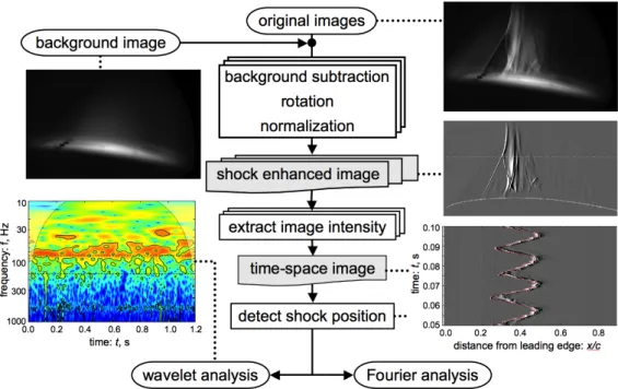
The acquired images were post-processed to analyze the shock oscillation. Figure 3 shows the flowchart of the image processing. This processing mainly consists of three parts: shock enhance-ment, conversion of a time-series image into a time-space map, and Fourier and wavelet analyses of a shock trajectory. Details on each process are discussed in the following sections.
3.1
Shock-wave Enhancement
The upper right side figure in Fig. 3 shows typical unprocessed flow images. The center por-tion of the image captures the shock waves established on the upper side of the airfoil. The flow images were subtracted by a blank (background) image taken for wind off pixel by pixel. The background-subtracted images were rotated, as the AoA became zero. Each rotated image was normalized as the spatial-averaged intensity became zero and the spatial-standard deviation of the intensities became unity. After these processing, the shock wave was enhanced by multiplying the processed image by its gradient in chordwise-direction pixel by pixel. The image intensities on the shock region were much higher than those on the other regions. The image gradients on the shock region were also high compared to the other regions, because the shock region was thin. Therefore, the product of the image intensity and its gradient enhanced the shock wave region as shown in the middle right side figure in Fig. 3. As a result, the shock region is indicated by the brightest line in this figure. Note that the model position was superimposed to the processed image by the white line in this figure.
3.2
Shock-trajectory Extraction
The image intensities were extracted along x/c at a certain y/c from a time-series image and were remapped into x-t diagram. A typical x-t diagram is shown in the lower right side figure in
Fig. 3. The shock trajectory was traced by maximum signal point in each time, as shown by the red line in this figure. These processes accurately extracted the shock motion.
3.3
Fourier and Wavelet Analyses
The shock trajectory extracted from a time-series image was analyzed by Fourier and wavelet analyses. Fourier analysis extracted dominant frequency of the shock oscillation and its amplitude. The Fourier coefficients were calculated by FFT algorithm in Matlab software. Spectral averaging reduced the random noise in the frequency domain. This was done by breaking the input data into many segments. In this study, we acquired the images during 1.2 s in a single experiment. These data were divided into eleven segments of 0.2 s with 50% segmentation overlap. From each seg-ment, Fourier spectra were calculated and were averaged to reduce the spectral noise. Because the data length for Fourier analysis was 0.2 s, frequency resolution was 5 Hz.
Fourier analysis decomposes time-series data into periodic functions having various cycles. This analysis well extracts dominate cycle speed, strength and phase in the frequency space. This analysis, however, loses time information. Fourier analysis is difficult to extract how dominant cycles vary in time for non-periodic signals. On the other hand, wavelet analysis decomposes time-series data into frequency-time space and is able to determine both dominant cycles of the data and how those dominant signals vary in time. Therefore, we applied wavelet analysis to the non-periodic shock motion which mainly appeared for the cases with VGs. Torrence and Compo (1998) provide a very useful practical guide to wavelet analysis including statistical significance testing. We followed their guidance to evaluate wavelet power spectrum.
In continuous wavelet transforms (CWT), the wavelet coefficients T(a,b) are evaluated by the convolution of a signal S(t) and a wavelet function ψ(t).
! T a
(
,b)
= S t( )
1 a" t#b a $ % & ' ( ) dt*
(1) where  ̄ indicates the complex conjugate. The parameter a controls the scale of the wavelet function and the parameter b controls the position (time shift) of the wavelet function. A Morlet wavelet function was used to estimate wavelet power spectrograms in this study. The Morlet wavelet function is one of the popular wavelet functions used in practice.
"
( )
t
=
#
$1 4where ω0 is the central frequency of the Morlet wavelet function. This parameter determines the
maximum scale of the analyzing wavelet. The ω0 was set to be 12. For this value, wavelet
frequen-cy f’ (=1/a) corresponds to Fourier frequency f as following the equation:
!
f = "0+ 2+"0
2
4# f $ = 1.92f $ (3)
In addition to evaluate the wavelet coefficient, background spectral noise was estimated and used for statistical significance testing. To determine significance levels, a background spectrum should be chosen appropriately. For the present case, an appropriate background spectrum could be modeled by red noise (increasing power with decreasing frequency). The lag-1 autoregressive process with Gaussian noise yielded the background spectrum PBG as follow:
! PBG
( )
f = 1"#2 1+#2"2#cos 2(
$f)
(4)where αis the lag-1 autocorrelation of S(t). This model well reproduced with the experimental results, as will be mentioned in Scet. 4.3. When a spectral peak of the measured data is 3-times higher than the background spectrum, the peak is assumed to be true feature in the spectrum at 95% confidence level. Details in the significant test for wavelet spectrum are in Torrence and Compo (1998).
4
Results and Discussions
4.1
Typical Schlieren Images and Flow Three Dimensionality
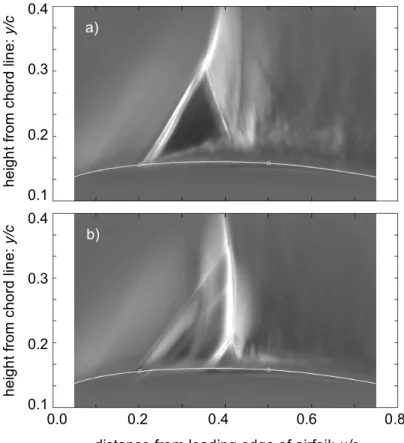
Figure 4 shows typical focusing-schlieren images with and without VGs at AoA = 6°. Figure 4a is the image without VGs when the shock wave traveled upstream. Figure 4b is the image with VGs. The interval between adjacent VGs was 12 mm (DVG/HVG = 10). For both cases, only back-ground subtraction and image rotation were applied. The model surfaces were superimposed on the processed images by the white lines. As will be mentioned in Sect. 4.2, the shock-buffet occurred at this AoA = 6° when the VGs were not installed. The installation of the VGs prevented from the buffet at this AoA.
For the case without VGs, the shock wave strongly interacted with the turbulent boundary layer on the upper surface. The positive pressure gradient due to the shock wave induced the boundary layer separation. The very large λ-type shock wave was generated by the SWBLI as
shown in Fig. 4a. The triple point of the λ-type shock reached at y/c ~ 0.3. The foot of λ-shock went upstream of x/c ~ 0.2. The strong SWBLI resulted in the shock-oscillation.
When the shock wave traveled upstream, very large λ-shock and boundary-layer separation appeared as shown in Fig. 4a. On the other hand, when the shock wave traveled downstream, the shape of the shock wave changed form λ-type to normal shock and the flow separation disappeared. For both shock-traveling cases, many pressure waves propagated from the downstream of the shock wave to the upstream. These waves merged with the shock wave and seem to drive the shock-oscillation (Yamaguchi et al. 2015).
Installation of VGs reduced SWBLI and made the separation smaller as shown in Fig. 4b. The small λ-shock appeared at x/c ~ 0.4. The amplitude of the shock-oscillation was quite smaller than that without VGs. Two left running shock waves also appear from the upper surface at x/c ~ 0.2 due to the installation of the VGs. These waves impinges into the λ-shock at y/c = 0.25 and 0.35.
Figure 4b shows not only the flow structures but also the importance of the narrow DOF to reduce capturing the unwanted structure. Figure 4b shows very blurred wave at x/c ~ 0.32 in
Fig. 4 Typical focusing schlieren images of the flow on the upper side of a supercritical airfoil at AoA = 6°: a) without VGs and b) with VGs. Open circulars on the surface of the airfoil indicate x/c = 0.2 and 0.5.
hei gh t fr om c hor d li n e: y/ c 0.4 0.3 0.2 0.1 0.0 b) a) hei gh t fr om c hor d li n e: y/ c 0.4 0.3 0.2 0.1 0.0 0.0 0.2 0.4 0.6 0.8 distance from leading edge of airfoil: x/c
tion to the clear ones at x/c ~ 0.4. This blur wave overlapped on the clear left running waves from the VGs. This blurred region was caused by the shock wave sited on the region out of focus. The VGs were not installed near the both sidewalls (see Fig. 1). The shock wave near the sidewall might propagate upstream compared with that in the center part of the airfoil. In addition, flow three-dimensionality became remarkable when the interval between the VGs increased. The flow structures just behind VGs could be different from those at the middle points between VGs. Thus, the narrow DOF is necessary to investigate the flow structures in detail for the cases with VGs. The focusing schlieren imaging is better suited for the buffet researches with VGs, compared with the conventional schlieren.
4.2
Unsteady Shock Wave Motions
Figures 5 and 6 show the time-space shock trajectories extracted at y/c = 0.3. We chose this height of y/c = 0.3, because the maximum height of the triple point of the λ-shock was below this position. The horizontal axis is x/c and the vertical axis is the time from start of the data acquisi-tion. These time-space maps were reconstructed from the time-series images processed only by background subtraction and image rotation. The bright line, or sometimes broad band, indicate the shock trajectory in these figures. These time-space maps show not only the shock wave motion but also the upstream propagating pressure waves. The time-space maps clearly show the left-running stripe patterns downstream of the shock trajectories shown by the bright lines in Figs. 5 and 6. The presence of the stripe patterns indicates the pressure waves were periodically generated and trav-eled upstream. Please refer to Kouchi (2017) for the details on the analysis of the upstream propa-gating pressure waves.
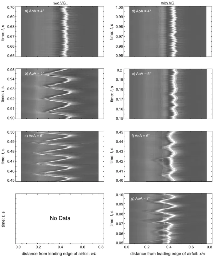
Figure 5 shows the shock motions for various AoA conditions and the effects of the installa-tion of VGs on them. The left figures are the trajectories without VGs and the right ones are those with VGs, respectively. The interval DVG/HVG was 10. The shock oscillations without VGs were quite periodic for all AoA conditions. Especially for high AoA ≥ 5°, the amplitude of the oscilla-tion was much larger than that at AoA = 4°. Such the type of the shock-oscillaoscilla-tion is usually referred as “shock-buffet”. In the buffet, both the cycle speed and amplitude of the oscillation increased with increasing AoA. Even without the buffet, the shock wave slightly oscillated. Its cycle speed was remarkably higher than those for the buffet cases.
Fig. 5 Typical shock motions at various AoA and the effects of the installation of VGs on it. The inter-val between the VGs is DVG/HVG = 10.
0.70 0.69 0.68 0.67 0.66 0.65 0.95 0.94 0.93 0.92 0.91 0.90 0.50 0.49 0.48 0.47 0.46 0.45 0.45 0.44 0.43 0.42 0.41 0.40 1.00 0.99 0.98 0.97 0.96 0.95 0.10 0.09 0.08 0.07 0.06 0.05 0.2 0.19 0.18 0.17 0.16 0.15 tim e : t , s
No Data
tim e : t , s tim e : t , s tim e : t , s tim e : t , s tim e : t , s tim e : t , s tim e : t , s w/o VG with VG a) AoA = 4° b) AoA = 5° c) AoA = 6° d) AoA = 4° e) AoA = 5° f) AoA = 6° g) AoA = 7° 0.0 0.2 0.4 0.6 0.8 distance from leading edge of airfoil: x/c0.0 0.2 0.4 0.6 0.8 distance from leading edge of airfoil: x/c
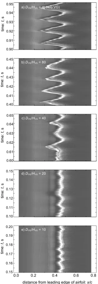
Fig. 6 Effects of the interval between the VGs on the shock oscillations. 0.15 0.14 0.13 0.12 0.11 0.10 0.20 0.19 0.18 0.17 0.16 0.15 tim e : t , s 0.0 0.2 0.4 0.6 0.8 distance from leading edge of airfoil: x/c
tim e : t , s tim e : t , s 0.45 0.44 0.43 0.42 0.41 0.40 tim e : t , s 0.65 0.64 0.63 0.62 0.61 0.60 tim e : t , s e) DVG/HVG = 10 d) DVG/HVG = 20 c) DVG/HVG = 40 b) DVG/HVG = 80 0.95 0.94 0.93 0.92 0.91 0.90 a) DVG/HVG = ∞ (w/o VG)
Installation of VGs seems not to affect the shock oscillation at AoA = 4°. This was drastically changed for high AoA ≥ 5°. At AoA = 5°, the installation of VGs greatly reduced the amplitude of the shock oscillation. The high frequency component observed at AoA = 4° became remarkable with installing the VGs at this AoA. Thus, the installation of VGs controlled the buffet. However, the low frequency component of the shock oscillation was still included in Figs. 5e-5g, for exam-ple t = 0.15-0.18 s in Fig. 5e, though its amplitude was quite small compared with those without VGs. With increasing AoA, the amplitude of the low frequency oscillation increased. The cycle and amplitude of the shock oscillation became irregular.
Figure 6 shows the effects of DVG on the shock motions. The angle of attack was fixed to be 5° where the shock-buffet occurred in the case without VGs. With decreasing DVG, the amplitude of the low frequency component due to the shock-buffet decreased and its cycle became irregular. Comparison of Figs 6a with 6b indicates that the shock oscillation was less affected by installing the VGs with their interval of DVG/HVG = 80. On the other hand, Figure 6c shows that the shock motion was quite non-periodic at DVG/HVG = 40. The oscillation having the similar frequency and amplitude to the shock-buffet intermittently appeared at DVG/HVG = 40. Figure 6d shows that the amplitude of the shock oscillation at DVG/HVG = 20 was greatly reduced by installing the VGs. From these two figures, the buffet onset should be between DVG/HVG of 20 and 40 at this AoA = 5°. At much shorter interval of DVG/HVG = 10, the high frequency component which was observed in the case without the buffet became remarkable. The low frequency component having the similar frequency to the buffet oscillation, however, was still included though its amplitude was small in this case.
4.3
Fourier Spectrum and Its Limitation
Fourier analysis extracted the dominant frequency and its amplitude extracted from each shock trajectory. Figures 7 and 8 show the power spectrum density (PSD) functions of the shock oscillations and the effects of the installation of the VGs on them. The background spectra esti-mated by Eq. 4 are also shown by the dashed lines in these figures. Before establishing the buffet, the estimated background spectra (Figs 7a and 7d) well agreed with the measured PSD functions in all frequency regions. On the other hand, after establishing the buffet, some discrepancy appeared between the estimated and measured data at very low frequency, for example f < 30 Hz in Fig. 7c. This discrepancy was caused by the frequency component of the buffet oscillation. The
overesti-mation of the background spectra in very low frequency region, however, has little noticeable
effect on the significance region of the wavelet spectrograms (see Appendix).
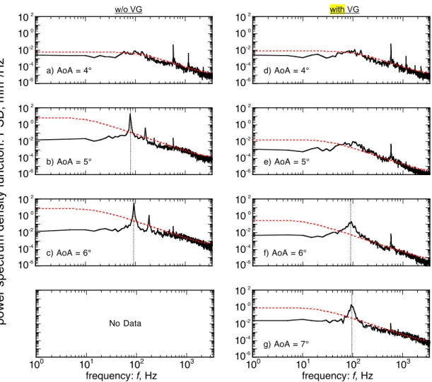
Figure 7 shows the PSD functions with and without VGs for various AoA. For the case with VGs, the interval DVG/HVG was 10. Referring first to the cases without VGs, the energy containing the shock oscillation at AoA = 4° was globally lower than those at AoA ≥ 5°, because the buffet was not established for this case. A spectral peak, however, is observed at 585 Hz. In addition, a spectral bump is observed between 40 and 200 Hz. The amplitude of this bump increased with increasing AoA and a remarkable spectral peak emerges at a low frequency near 100 Hz where the bump was detected. These peaks corresponded to the shock oscillation due to the buffet.
10-2 10-0 10-2 10-4 10-6 a) AoA = 4°
10-2 10-0 10-2 10-4 10-6 d) AoA = 4°
10-2 10-0 10-2 10-4 10-6 b) AoA = 5°
10-2 10-0 10-2 10-4 10-6 e) AoA = 5°
10-2 10-0 10-2 10-4 10-6 c) AoA = 6°
10-2 10-0 10-2 10-4 10-6 f) AoA = 6° 100 101 102 103 No Data frequency: f, Hz
100 101 102 103 10-2 10-0 10-2 10-4 10-6 g) AoA = 7° frequency: f, Hz
Fig. 7 Fourier spectra of shock motion with and without VGs and their estimated background spectra using lag-1 autocorrelation: DVG/HVG = 10.
p
o
w
e
r
sp
e
ct
ru
m
d
e
n
si
ty
fu
n
ct
io
n
:
P
S
D
,
m
m
2/H
z
w/o VG with VG10-2 10-0 10-2 10-4 10-6 a) DVG/HVG = 10 10-2 10-0 10-2 10-4 10-6 b) DVG/HVG = 20 10-2 10-0 10-2 10-4 10-6 c) DVG/HVG = 40 10-2 10-0 10-2 10-4 10-6 c) DVG/HVG = 80 100 101 102 103 10-2 10-0 10-2 10-4 10-6 e) DVG/HVG = ∞ frequency: f, Hz
Fig. 8 Effect of DVG on Fourier spectra of shock motion: AoA
= 5°. Estimated background spectra using lag-1 autocorrela-tion are also shown by dashed lines.
p
o
w
e
r
sp
e
ct
ru
m
d
e
n
si
ty
fu
n
ct
io
n
:
P
S
D
,
m
m
2/H
z
Comparison of Figs 7b and 7c shows the buffet frequency (fB) is sensitive to AoA. The fB was 80 Hz at AoA = 5° and this increased to 95 Hz at AoA = 6°. For all case, the PSD functions con-tain higher harmonic ones. These higher harmonic oscillations determined the shape of the shock trajectory. In our experiments, the higher harmonic oscillations changed the shape of the shock trajectory from sinusoidal wave to triangle wave as shown in Figs. 5b and 5c.
These results in terms of fB and its trend with AoA are similar to those reported by Jacquin et al (2009) and other researchers. Jacquin et al (2009) obtained PSD from unsteady pressure measurements with dynamic pressure transducers installed in OAT15A airfoil with c = 230 mm in
continuous closed-circuit transonic S3Ch wind tunnel. The scale of our airfoil was similar to that of their model, so a similar fB was observed in both experiments after establishing the buffet. Inter-estingly, a spectral peak was also observed near 600 Hz without the buffet in their experiment at AoA = 3°. This is similar to our experiment as shown in Fig. 7a. Detail investigation of the schlieren movies revealed that this shock oscillation synchronized with the incident pressure waves from downstream side. This incident pressure wave could be generated by two reasons: One is the flow itself and the other is the downstream configuration of the wind tunnel facility. We believe this incident pressure waves were originated from flow itself such as a trailing edge vor-tices, because this higher spectral peak was observed in the two different wind tunnels. Hermes et al. (2013) numerically investigated the upstream traveling pressure waves over a supercritical airfoil in a cruise condition at AoA = 0°. Weak pressure waves were generated in the vicinity of the trailing edge of the airfoil associated with the large-scale structures in the boundary layer. These weak pressure waves gathered with traveling upstream and induced periodic shock forma-tion. Similar trends were observed in our experiment at AoA = 0°. Shock formation frequency in our experiment was similar to the higher significant frequency of 585 Hz observed before estab-lishing the buffet at AoA = 4°. This implied that the higher spectral peak was originated from the Kutta waves.
Referring second to the cases with VGs, there is no remarkable change between with and without VGs at AoA = 4°. With increasing AoA, the spectral bump observed between 40 and 200 Hz gradually emerged to be the spectral peak due to the shock-buffet. The peak power of fB in the case with VGs at AoA = 7° was quite smaller than that without VGs at AoA = 6°. In addition, the power containing in higher frequency increased with increasing AoA. The similar trend was ob-served with changing the interval between
the VGs. Figure 8 shows the PSD func-tions for the various DVG. The spectral bump gradually emerged with increasing
DVG. The frequencies where the maximum powers were observed near fB seemed to be varied with changing DVG.
Thus, the Fourier analysis well ex-tracted the characteristics of the shock
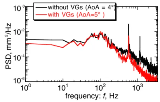
without VGs (AoA = 4°) with VGs (AoA=5° ) 100 101 102 103 10-0 10-2 10-4 10-6 PSD, mm 2 /Hz frequency: f, Hz
Fig. 9 Comparison of PSD with and with-out VGs before establishing the buffet.
motion having the periodic oscillation. Even for the cases with VGs, the analysis captured some trends due to the VGs, AoA and DVG. The Fourier analysis, however, was not enough to extract the characteristics of the shock oscillation in the cases with VGs, because the shock oscillations for some cases with VGs were not periodic (see Figs 5f, 5g and 6c). The Fourier analysis is difficult to accurately extract the characteristics of the non-periodic motions.
Figure 9 shows the comparison of PSD functions with and without VGs before establishing the shock-buffet. There is no remarkable difference of the PSD functions between with and with-out VGs in low frequency regime around 100 Hz. However, the shock oscillation with VGs at AoA = 5°, where the buffet was controlled by installing the VGs, had a low frequency component like a buffet (see Fig. 5e). The Fourier analysis does not well recognize this low frequency oscilla-tion, because the oscillation intermittently appeared in the cycle. Such a non-periodic component is difficult to be classified by using the Fourier analysis. Therefore, we applied the wavelet analysis to the shock trajectories.
4.3
Wavelet Spectrogram
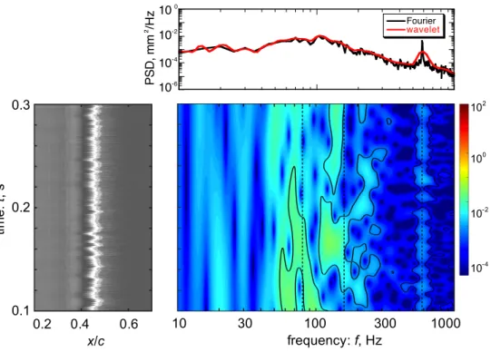
Figure 10 shows a typical wavelet power spectrogram of the shock trajectory in the case with VGs at AoA = 5°. The interval DVG/HVG was 10. The wavelet power was indicated by color con-tours in the lower right side figure of Fig. 10. The horizontal axis is the Fourier frequency convert-ed from the wavelet frequency using Eq. 3 and the vertical axis is the time after starting the image acquisition, respectively. The thick contour encloses the regions of greater than 95% confidence level for the background spectrum. Dashed lines shows fB observed without VGs. The left figure indicates the shock trajectory corresponded to the spectrogram and the upper right figure is the wavelet PSD function evaluated by integrating the power through the time direction in the wavelet spectrogram. The wavelet PSD function is compared with the Fourier one.
For this case, the installation of the VGs controlled the shock-buffet. The upper right side fig-ure of Fig. 10 shows the shock wave mainly oscillated with the high frequency synchronized with the incident pressure waves as mentioned in Figs. 5a and 5d. The shock oscillation, however, in-termittently included the low frequency component like the shock-buffet, though its amplitude was quite small. The low frequency component was remarkable for 0.1 ≤t≤ 0.2 as shown in the left figure of Fig. 10. The wavelet spectrogram with the significant test well represented these charac-teristics. The significant spectral band is observed around f = 600 Hz through the whole test
dura-tion. In addition, the significant spectral bans are observed around fB and its second harmonic one for 0.1 ≤t≤ 0.2. Thus, the wavelet analysis is able to extract such non-periodic features from the shock oscillation.
Figure 11 shows the wavelet power spectrograms with and without VGs for various AoA. The left column indicates the spectrograms without VGs and the right column indicates those with VGs (DVG/HVG = 10). The dashed lines in Fig. 11 show fB observed without VGs at the same AoA and the higher frequency of 585 Hz. Note that lighter shade areas in these figures are the cones of influence where edge effects might distort the spectrograms.
Referring first to the cases without VGs in the left column of Fig. 11, the features of the spectrograms coincide with those of Fourier spectra as shown in Figs. 7a-7c. The significant spectral band is observed around f = 600 Hz at AoA = 4°. This corresponds to the spectral peak at 585 Hz in Fig. 7a. After establishing the buffet, two significant spectral bands appeared around 100 Hz and 200 Hz in Figs. 11b and 11c. These correspond to the spectral peaks due to the buffet at f = 80 Hz and 160 Hz in Fig. 7b, and 95 Hz and 190 Hz in Fig. 7c, respectively. Both the oscillations at f ~ 600 Hz and at f ~ 100 Hz are quite periodic because the significant bands are observed in all the measuring time. In addition to these spectral bands, a few significant spots are observed at AoA = 4° between f = 60 Hz and 200 Hz before establishing the buffet. We believe that these intermittent spots were the origin of the buffet.
Fourier wavelet 10-0 10-2 10-4 10-6 PSD, mm 2 /Hz
Fig. 10 Typical wavelet spectrogram corresponded to shock trajectory in the case with VGs: DVG/HVG = 10 and AoA = 5°.
10 30 100 300 1000 frequency: f, Hz 0.2 0.4 0.6 x/c 0.3 0.2 0.1 tim e : t , s 102 100 10-2 10-4
Referring second to the cases with VGs in the right column of Fig. 11, there is no remarkable change in the wavelet spectrogram at AoA = 4° between with and without VGs. The installation of the VGs was no effects on the shock motion before establishing the buffet. On the other hand, the significant spectral bands around f = 100 Hz and 200 Hz disappeared with installing the VGs for AoA ≥ 5°. Instead of this, the significant spectral spots appeared between f = 60 Hz to 200 Hz. The
Fig. 11 Wavelet power spectrogram with and without VGs for various AoA =5°: DVG/HVG = 10. 102 100 10-2 10-4 10 30 100 300 1000 frequency: f, Hz 1.2 1.0 0.8 0.6 0.4 0.2 0.0 tim e : t , s 10 30 100 300 1000 frequency: f, Hz 1.2 1.0 0.8 0.6 0.4 0.2 0.0 1.2 1.0 0.8 0.6 0.4 0.2 0.0 1.2 1.0 0.8 0.6 0.4 0.2 0.0 tim e : t , s tim e : t , s tim e : t , s 1.2 1.0 0.8 0.6 0.4 0.2 0.0 tim e : t , s 1.2 1.0 0.8 0.6 0.4 0.2 0.0 1.2 1.0 0.8 0.6 0.4 0.2 0.0 1.2 1.0 0.8 0.6 0.4 0.2 0.0 tim e : t , s tim e : t , s tim e : t , s b) AoA = 5° e) AoA = 5° a) AoA = 4° d) AoA = 4° c) AoA = 6° f) AoA = 6° g) AoA = 7° without VGs with VGs No Data
Fig. 12 Wavelet power spectrograms for various DVG/HVG: AoA =5°. 102 100 10-2 10-4 10 30 100 300 1000 frequency: f, Hz 1.2 1.0 0.8 0.6 0.4 0.2 0.0 tim e : t , s 1.2 1.0 0.8 0.6 0.4 0.2 0.0 1.2 1.0 0.8 0.6 0.4 0.2 0.0 1.2 1.0 0.8 0.6 0.4 0.2 0.0 tim e : t , s tim e : t , s tim e : t , s 1.2 1.0 0.8 0.6 0.4 0.2 0.0 tim e : t , s a) DVG/HVG = ∞ (w/o VG) d) DVG/HVG = 20 c) DVG/HVG = 40 b) DVG/HVG = 80 e) DVG/HVG = 10
rate of appearing the 95% confidence regions at AoA = 5° was remarkably higher than those at AoA = 4°. Their amplitude were also higher than those at AoA = 4°. These implied that the instal-lation of the VGs did not perfectly suppress the low frequency shock-oscilinstal-lation due to the buffet.
Near the onset of the buffet as shown in Fig. 11f, the shock oscillation included the high am-plitude oscillation at f = 60~80 Hz, which was lower than fB (= 95 Hz) at this AoA = 6°. The bandwidth became narrow with increasing AoA to 7°. This indicates that the shock oscillation became periodic at AoA = 7°.
Figure 12 shows the effects of DVG/HVG on the wavelet spectrograms. The angle of attack was 5°. The dashed lines in Fig. 12 shows fB of 80 Hz and its second harmonic of 160 Hz observed without VGs at the same AoA. The higher significant frequency of 585 Hz is also indicated by the dashed lines.
At DVG/HVG = 80, the buffet oscillation was nearly periodic as similar to that without the VGs (DVG/HVG = ∞). Its amplitude, however, was lower than that without the VGs. The installation of the VGs affects the SWBLI even at such the large interval of DVG/HVG = 80. The shock motion was quite different for the cases between at DVG/HVG = 80 and 40. At DVG/HVG = 40, the signifi-cant regions spread at lower frequencies than fB (= 80 Hz). This case was onset of the shock-buffet. Figures 12c and 11f imply the cycle of the shock oscillations near the onset of the buffet became slower than those with the buffet.
For DVG/HVG≤ 20, the shock oscillation near fB appeared intermittently. The significant spots appeared between fB and its second harmonic. Comparison of Figs. 12d and 12e shows that the intermittency of appearing the significant spots between fB and its second harmonic was less af-fected by DVG/HVG. The amplitude of the significant regions was slightly decreased with decreas-ing DVG/HVG. Thus, the wavelet analysis with the significance test gave quantitative measure of change in the non-periodic shock motions, mainly caused by installing the VGs, as well as the periodic shock motions.
5
Conclusion
We experimentally investigated the effects of the installation of the VGs on two-dimensional shock-buffets. The flowfields around a supercritical airfoil with and without VGs were visualized at Re = 5 x 10⁶ by using the fast-framing focusing schlieren. The focusing schlieren visualizations revealed that the shock-buffet appeared at AoA ≥ 5° without VGs. The remarkable shock
oscilla-tion due to the buffet disappeared with installing the VGs even for much higher AoA of 6°. Flow three-dimensionality became also remarkable with installing the VGs even for the two-dimensional wing experiments. Narrow DOF in the present visualization system was key to accu-rately capture the shock oscillations for the cases with the VGs.
Based on the time-series schlieren images, we analyzed the shock motions by using Fourier and wavelet analyses. Fourier analysis well extracted the buffet frequency and its amplitude for the periodical shock oscillations observed mainly in the cases without the VGs. The buffet frequency was 80 Hz in the present airfoil at AoA = 5°. This increased to 95 Hz with increasing AoA = 6°. The Fourier analysis, however, is difficult to extract the characteristics of the shock oscillation including non-periodic components which observed mainly in the cases with VGs.
The wavelet analysis using Morlet wavelet function successfully extracted the characteristics of the non-periodic shock oscillation appearing in the cases with VGs. The wavelet spectrograms show that the 95% confidence regions appeared intermittently between the buffet frequency and its second harmonic when VG controlled the shock-buffet. Its amplitude was quite lower than those in the buffet cases. The rate of appearing the confidence regions increased with increasing both AoA and DVG/HVG. The power of this component also increased with increasing them. At the onset of the buffet, the dominated frequency of the shock motion shifted toward to a lower frequency than the buffet frequency in the case with VGs. Thus, combination of the fast-framing focusing schlieren visualization and the wavelet analysis of them help to develop our understanding of the shock-buffet and the effects of the installation of VGs.
Appendix
A.
Effect of Buffet Frequency on Estimated Background Spectra
Equation 4 used the lag-1 autocorrelation αto estimate background spectrum. After establish-ing the buffet, α increased compared with that before establishing the buffet. This resulted in the overestimation of background at f << fB. Figure A1 shows the typical effect of the frequency com-ponent due to the buffet on the estimated background spectrum in the case with VGs at AoA = 6°. The interval DVG/HVG was 10. In this case, the shock oscillation was non-periodic and the buffet oscillation intermittently generated as shown in Fig. 5f. The red dashed lines are the background spectrum using α estimated from non-filtered shock trajectory data which includes the frequency
component due to the buffet. On the other hand, the blue ones are using α estimated from band-stopped filtered data from 50 Hz to 150 Hz, which have no frequency component due to the buffet. The background spectrum using the filtered data well agrees with the measured data even in the
very lower frequency region.
Therefore, we conclude that the overestimation of the background spectra at very low frequency is caused by the frequency component due to the buffet.
Figure A2 shows the effects of this overestimation on the significant regions in the wavelet spectrogram. The significance regions were determined by the background spectrum using α estimated from the non-filtered shock trajectory data for the upper figure, and those were from
the filtered data for the lower figure, respectively. Although the significant regions are slightly extended for the background estimated from the filtered data, overall the overestimation has no remarkable effect on our conclusion. The background spectrum estimated from the filtered data might be appropriate as the background spectrum. The buffet frequency, however, is difficult to determine for the cases with VGs or the buffet onset. Therefore, we chose the non-filtered data to estimate the background.
nonFiltered (!=0.990) Filtered (!=0.952) 100 101 102 103 10-2 10-0 10-2 10-4 10-6 f) AoA = 6° PSD, mm 2 /Hz frequency: f, Hz
Fig. A1 Effect of frequency component due to buffet on the estimated background spectrum.
Fig. A2 Effects of the overestimation of the back-ground at very low frequency region on the signifi-cant regions in the wavelet spectrogram.
10 30 100 300 1000 frequency: f, Hz 1.2 1.0 0.8 0.6 0.4 0.2 0.0 tim e : t , s 1.2 1.0 0.8 0.6 0.4 0.2 0.0 tim e : t , s 102 100 10-2 10-4
Acknowledgments
This work was partially supported by JSPS KAKENHI Grant-in-Aid for Scientific Research (B) 15H04199. The authors appreciate for supporting of the wind tunnel ex-periments by JAXA Aerodynamics Research Unit.References
Braslow AL and Knox EC (1958) Simplified Method for Determination of Critical Height of Distributed Roughness Particles for Boundary-layer Transition at Mach Number from 0 to 5. NACA TN-4363.
Crouch JD, Garbaruk A, Magidov D, Travin A (2009) Origin of Transonic Buffet on Aero-foil. J. Fluid Mech. 628: 357–369. [DOI:10.1017/S0022112009006673]
Harris CD (1990) NASA Supercritical Airfoils (a Matrix of Family-Related Airfoils). NASA TP-2969.
Hermes V, Klioutchnikov I, Olivier H (2013) Numerical investigation of unsteady wave
phe-nomena for transonic airfoil flow. Aero. Science and Tech. 25: 224-233. [DOI: 10.1016/j.ast.20
12.01.009]
Ito Y, Yamamoto K, Kusunose K, Koike S, Nakakita K, Murayama M (2016) Effect of Vortex Generators on Transonic Swept Wings. J. Aircraft (in printing)
Jacquin L, Molton P, Deck S, Maury B, Soulevant D (2009) Experimental Study of Shock Oscillation Over A Transonic Supercritical Profile. AIAA J. 49(7): 1985-1994. [DOI: 10.2514/1.30 190]
Koike S, Sato M, Kanda H, Nakajima T, Nakakita K, Kusunose K, Murayama M, Ito Y, Ya-mamoto K (2013) Experiment of Vortex Generators on NASA SC(2)-0518 Two Dimensional Wing for Buffet Reduction. APISAT-2013 05-08-2.
Koike S, Nakakita K, Nakajima T, Koga S, Sato M, Kanda H, Kusunose K, Murayama M, Ito Y, Yamamoto K (2015) Experimental Investigation of Vortex Generator Effect on Two- and Three-Dimensional NASA Common Research Models. AIAA paper 2015-1237.
Kouchi T, Goyne C, Rockwell R, McDaniel J (2015) Focusing-schlieren Visualization in A Dual-mode Scramjet. Exp. Fluids 56(211). [DOI: 10.1007/s00348-015-2081-9]
Kouchi T, Yamaguchi S, Yamashita Y, Yanase S, Koike S (2017) Modified Lee’s Transonic Buffet Mechanism Inspired with Fast-framing Focusing-schlieren Visualization. AIAA paper (to be presented in AIAA Scitech 2017).
Kozaki N, Kato H, Nakakita K, Kanazaki M (2015) Optimum Layout of Vortex Generators for Upper Surface of Wing Using Efficient Global Optimization. Trans. JSME 81(830). [DOI: 10.1 299/transjsme.15-00188] (in Japanese)
Kusunose K, Yu NJ (2003) Vortex Generator Installation Drag on an Airplane near Its Cruise Condition. J. Aircraft 40(6): 1145-1151. [DOI: 10.2514/2.7203]
Lee BHK (2001) Self-sustained shock oscillations on airfoils at transonic speeds. Prog. Aero. Sciences 37: 147-196. [DOI:10.1016/S0376-0421(01)00003-3]
Molton P, Dandois J, Lepage A, Brunet V, Bur R (2013) Control of Buffet Phenomenon on a Transonic Swept Wing. AIAA J. 51(4): 761-772. [DOI: 10.2514/1.J051000]
Namura N, Obayashi S, Jeong S (2016) Efficient Global Optimization of Vortex Generators on a Supercritical Infinite Wing. J. Aircraft (in printing) [DOI: 10.2514/1.C033753]
NAL Second Aerodynamics Division (1982) Construction and Performance of NAL Two-Dimensional Transonic Wind Tunnel. NAL TR-647T.
NAL Two-dimensional Transonic Wind Tunnel Laboratory (1999) Revitalization of NAL Two-Dimensional Transonic Wind Tunnel. NAL TM-744. (in Japanese)
Sato M, Kanda H, Nagai S (2010) Effects of Sidewall Boundary Layer Suction in Two di-mensional Airfoil Testing. JAXA-RM-10-006. (in Japanese)
Sawada H (1978) A General Correction Method of the Interference in 2-Dimensional Wind Tunnels with Ventilated Walls. Transactions of the Japan Society for Aeronautical and Space Sciences 21(52): 57-68.
Schlichting H (1979) Boundary-layer Theory (7th ed.). McGraw-hill, New York: 378-407. Settles GS (2001) Schlieren and Shadowgraph Techniques. Springer-Verlag, New York: 77-96. [DOI: 10.1007/978-3-642-56640-0]
Stanewsky E, Baster D (1990) Experimental Investigation of Buffet Onset and Penetration on A Supercritical Airfoil at Transonic Speeds. AGARD CP-483: 4-1-4-11.
Sugioka Y, Numata D, Asai K, Koike S, Nakakita K, Nakajima T (2016) Polymer/Ceramic PSP with Reduced Surface Roughness for Unsteady Pressure Measurement in Transonic Flow. AIAA 2016-2018.
Titchener N, Babinsky H (2015) A Review of The Use of Vortex Generators for Mitigating
Shock-induced Separation. Shock Waves 25: 473–494. [DOI: 10.1007/s00193-015-0551-x]
Torrence C, Compo GP (1998) A Practical Guide to Wavelet Analysis. Bulletin of the Ameri-can Meteorological Society 79(1): 61-78.
Weinstein LM (2010) Review and Update of Lens and Grid Schlieren and Motion Camera Schlieren. Eur. Phys. J. Special Topics 182(1): 65-95. [DOI: 10.1140/epjst/e2010-01226-y]
Yamaguchi S, Kouchi T, Koike S, Nakajima T, Sato M, Kanda H, Yanase S (2015) Fast-framing Focusing Schlieren Visualization of Two-dimensional Wing Buffet. J. Japan Soc. Aero. Space Science, 63(4): 166-174. (in Japanese) [DOI: 10.2322/jjsass.63.166]
Zhao Z, Ren X, Gao C, Xiong J, Liu F, Luo S (2013) Experimental Study of Shock Wave Oscillation on SC(2)- 0714 Airfoil. AIAA 2013-0537.