Duration dependence test of rational speculative bubbles: a case study of the Hong Kong stock market

(1)

Christopher Gan (New Zealand), Gilbert V. Nartea (New Zealand), Dou Ling Ling (China), Baiding Hu (New Zealand)

Duration dependence test of rational speculative bubbles:

a case study of the Hong Kong stock market

Abstract

This study tests the presence of rational speculative bubbles in the Hong Kong stock market over a sample period from 1993-2008 using the duration dependence test. The duration dependence test shows no evidence of duration depen-dence, suggesting that the Hong Kong stock market did not exhibit rational speculative bubbles before (1993-1997) and after (1998-2008) the 1997 Asian financial crisis. The results also suggest that the tests are not sensitive to the choice of different models, monthly versus weekly runs of returns and equally- versus value-weighted portfolio in the Hong Kong stock market. The results imply that the stock prices could be a reflection of the market fundamentals.

Keywords: duration dependence test, speculative bubbles, stock markets.

JEL Classifications: G11, G14, G19.

Introduction

Duration dependence test has been widely applied to investigate the presence of rational speculative bubbles in real estate markets (Lavin and Zorn, 2001; Das, 2007), business cycles (Sichel, 1991; Zuehlke, 2003) and equity markets (McQueen and Thorley, 1994; Chan, McQueen and Thorley, 1998; Watana-palachaikul and Islam, 2007; Yu and Sze, 2003). However, most researchers who use the duration dependence test to test for the presence of the ra-tional speculative bubbles in focus on the US and other developing and emerging markets, but there are limited studies addressing the speculative bub-bles on the Hong Kong stock market.

Several researches have tested for the presence of speculative bubbles in the Hong Kong stock market with different testing approaches, but they present contradictory findings. For example, Yu and Sze (2003) conclude the existence of asset price bubbles in the Hong Kong stock market during 1974 to 2002 using the specification and co-integration tests. Their result is confirmed by Wu and Xiao (2008) who used the co-integration test. In contrast, Chan et al. (1998) provide no significant evidence of rational bubbles in the Hong Kong stock market during the period from 1975 to 1994 using the duration dependence test. Lehkonen (2010) reported mixed results using dura-tion dependence test in Chinese stock markets and China-related share indices in Hong Kong. The au-thor’s result shows the presence of rational bubbles in weekly data for both of the Mainland Chinese stock exchange share classes, but fail to detect bubbles using monthly data. Furthermore, bubbles are not detected in the Hong Kong Stock Exchange.

The Hong Kong stock market is also affected by the government handover to China in 1997. Investors

Christopher Gan, Gilbert V. Nartea, Dou Ling Ling, Baiding Hu, 2012.

believed that the stock market potential could be interfered by the Chinese government. However, there is no previous research that examines whether there are rational speculative bubbles for the 10 years after the handover. This study tests the pres-ence of rational speculative bubbles in the Hong Kong stock market using the duration dependence test developed by McQueen and Thorley (1994). Compared to previous studies, our study is the first study to test the behavior of individual stocks instead of the Hang Seng Index, and is also the first study to test the behavior of Hong Kong stock market that takes into account the government handover and Asian fi-nancial crisis simultaneously. The time periods used in previous studies were limited to 1990s, while our study extends the data period from 1993 to 2008 and takes into account the pre and post 1997 Asian finan-cial crisis. In addition, both weekly and monthly data are used. The test is conducted using both the Log-logistic and Weibull hazard models. Finally, although the duration dependence test is unique to the bubbles, because of the sensitivity of duration dependence, the results will be impacted by the choice of a sample period, the model and the use of data.

The remainder of the paper is organized as follows. Section 1 reviews the literature on duration depen-dence test of rational speculative bubbles in the Asian stock markets. Section 2 outlines the empiri-cal model and describes the data. Section 3 presents and discusses the results. The final section offers concluding remarks.

1. Literature review

(2)

presence of bubbles and no model misspecification (Blanchard and Watson, 1982; West, 1987). For ex-ample, McQueen and Thorley (1994) used diagnostic tests to investigate the rational speculative bubbles including autocorrelation, skewness and kurtosis as well as the duration dependence test with log-logistic function. The authors employed abnormal continuous-ly compounded real monthcontinuous-ly returns for both equalcontinuous-ly- and value-weighted portfolios of all New York Stock Exchange (NYSE) stocks from 1927 to 1991. Their results show evidence of skewness, kurtosis and autocorrelation which are consistent with bubbles. However, these attributes are not unique to bubbles, and dependence test is more discriminating.

The Asian stock markets were highly volatile during the 1997 Asian financial crisis period and there is speculation that the Asian markets contain bubbles. Chan et al. (1998) used monthly and weekly stock market returns of six Asian markets (Hong Kong, Japan, South Korea, Malaysia, Thailand and Taiwan) from 1975 to 1994, except for Korea and Malaysia which begins in 1977 to test for rational speculative bubbles. Although the return distributions of these markets exhibited positive autocorrelation, negative skewness and leptokurtosis consistent with rational speculative bubbles, evidence from duration de-pendence test does not support the existence of rational speculative bubbles except for Thailand using weekly returns.

Jirasakuldech, Emekter and Rao (2007) confirmed the result of Chan et al. (1998) in Thailand stock market, which shows strong evidence of rational speculative bubbles from 1975-2006, but with monthly returns. However, the sub-period results con-form to the presence of rational speculative bubbles in the pre-1997, but not in the post-1997. Watanapala-chaikul and Islam (2007) also conducted a study on rational speculative bubbles in the Thailand stock market using the Weibull hazard model. Their empiri-cal results show that rational speculative bubbles are present during the pre-crisis period (1992-1996). However, the authors’ results provide no evidence of rational speculative bubbles during the post crisis pe-riod (1997-2001), except for 1997 and 1999. These studies obtain relatively the same results of rational speculative bubbles in Thailand stock market.

Rangel and Pillay (2007) and Zhang (2003) used the log-logistic function to detect the presence of ra-tional speculative bubbles in Asian markets. Rangel and Pillay (2007) tested for stock price bubbles in the Singaporean stock market from 1975 to 2007. Using monthly excess returns, their results indicate no possibility of rational speculative bubbles. How-ever, using prices rather than excess real returns they show significant duration dependence. Zhang

(2003) applied duration dependence tests in the Chinese stock market, focusing on the Shanghai Composite Index and the Shenzhen Composite In-dex from 1991 to 2001. Together with the evidence of autocorrelation and leptokutosis, the results re-port positive duration dependence which is consis-tent with rational bubbles.

Haque, Wang and Oyang (2008) tested whether the Chinese equity prices were characterized by rational speculative bubbles from 1991 to 2007. By employ-ing weekly data from the Shanghai composite index and the Shenzhen composite index with both the Weibull hazard model and log-logistic hazard mod-el, the authors’ finding suggests that Chinese securi-ties prices experience some episodes of rational expectation bubbles during the sample period, which confirm the results of Zhang (2003) about Chinese stock markets.

Using both the Weibull and log logistic hazard models, Mokhtar, Md. Nassir and Hassan (2006) supported the existence of rational speculative bub-bles in the Malaysian stock market before (1994-1996) and after (1999-2003) 1997 Asian financial crisis. Mokhtar et al. also report that the size of bub-bles during the pre-crisis period is larger than those during the post-crisis period. Allen and Bujang (2009) also tested for bubbles in the Malaysian stock market during 1994-2001 using the same me-thods as Mokhtar et al. (2006) and also report the existence of speculative bubbles consistent with Mokhtar et al. Allen and Bujang (2009) also indi-cated that there is duration dependence in both posi-tive and negaposi-tive runs of abnormal returns. Consis-tent with their study, Chan et al. (1998) also found duration dependence in runs of negative excess re-turns in the Malaysian stock market. However, the authors argued that the negative duration depen-dence is driven by other reasons such as fads, but not by rational bubbles.

2. Data and methodology

(3)

Enterprise Market (GEM) are excluded from our study since the GEM was established in 1999, whose history is too short to be used in the analysis.

Delisted or dead companies during the testing pe-riod are excluded in our sample selection. “Zero-yield” stocks, those paying no dividends during the previous month, are also excluded from the sample

since dividend yields are included in the calculation of abnormal return, and Fama and French (1993) argue that the zero-yield stocks do not conform to any monotonic relation between dividend yield and expected return. Further deletion is applied if the stock is traded less than three months within a year as the data may not be significant for the analysis.

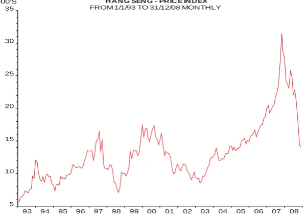
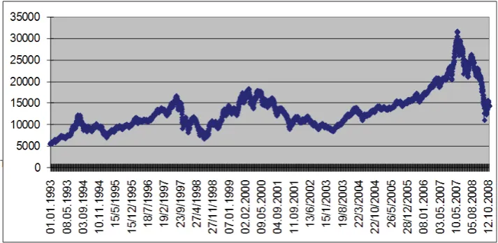
Source: Datastream.

Fig. 1. Hang Seng price index

Both monthly and weekly data are collected for the sample stocks. Both monthly and weekly returns are used for the following reasons. First, as documented in McQueen and Thorley (1994), monthly returns are less susceptible to noise, unlike weekly returns. Second, there is a lack of power in the shorter data series. Third, there is no clear indication about the length of a bubble hence we use both of the returns in order to increase the robustness of our results. In addition, Harman and Zuehlke (2004) revealed that the duration dependence test is sensitive to the use of monthly versus weekly runs of abnormal returns, which is supported by Lehkonen’s (2010) study. Duration dependence test is performed on continu-ously compounded monthly and weekly real returns and abnormal returns for both equally-weighted and value-weighted portfolios. Real returns are con-structed following the methods of McQueen and Thorley (1994), Jaradat (2009), Ali et al. (2009) and Jirasakuldech et al. (2006). Continuously compounded monthly and weekly nominal returns are created based on the total return index of individual stocks collected from Datastream. The nominal return for an individual stock is calculated by taking the first difference of the natural log of the total return in-dex. Monthly and weekly market rates of return are then constructed for both equally-weighted and

value-weighed portfolios of HKSE stocks listed on the Main Board.

To calculate real returns, continuously compounded monthly inflation rates are generated based on Hong Kong Consumer Price Index (CPI). Continuously compounded monthly inflation rates are calculated by taking the first difference of the natural log of the monthly CPI. Real returns are then calculated by subtracting continuously compounded inflation rates from continuously compounded nominal returns of the two portfolios.

The procedure in generating monthly continuously compounded abnormal returns is based on McQueen and Thorley (1994), Harman and Zuehlke (2004) and Ali et al. (2009) methods. The sequence of monthly abnormal returns is determined by the resi-duals from the regression of returns on its first three lags, the term spread, and the dividend yield. Divi-dend yield of individual stocks are collected from Datastream. To obtain abnormal returns, monthly value-weighted HKSE portfolio’s dividend yield is calculated. Consistent with Fama and French (1993) and McQueen and Thorley (1994), term spread is the difference in yield-to-maturity between long-term yield and short-long-term yield. In this study, 2-year Hong Kong Exchange Fund Notes are used as the long-term yield, and 1-month Hong Kong Interbank

H A N G SEN G - PR IC E IN D EX

FROM 1/1/93 TO 31/12/08 MONTHLY

93 94 95 96 97 98 99 00 01 02 03 04 05 06 07 08 000'S

(4)

Rates are used as short-term yield. Both yields are obtained from the Hong Kong Monetary Authority. Monthly abnormal returns are defined as the resi-duals from the following two regressions:

, 070 . 0 122 . 0 311 . 0 / 013 . 0 007 . 0 044 . 0 3 2 1 1 1 EW t EW t EW t EW t t t EW t R R R P D TERM R H (1) , 059 . 0 151 . 0 185 . 0 / 018 . 0 004 . 0 059 . 0 3 2 1 1 1 VW t VW t VW t VW t t t VW t R R R P D TERM R H (2)

where R_tEW and R_tVW are the real continuously com-pounded monthly returns on the equally- and value-weighted portfolios, respectively. TERM is the term spread, and D/P is the value-weighted dividend yield of all stocks.

The weekly continuously compounded abnormal returns is obtained following Chan et al. (1998) and Harman and Zuehlke (2004) methods. Weekly ab-normal returns are defined as the residuals from AR (4) model of weekly real returns. Chan et al. (1998) argue that AR (4) model is preferable to imposing a common mean, because it controls for short-term sources of autocorrelation. Thus, weekly abnormal returns are defined as the residuals from the follow-ing two regressions:

, 021079 . 0 051340 . 0 119069 . 0 080267 . 0 000625 . 0 4 3 2 1 EW t EW t EW t EW t EW t EW t R R R R R H ₍₃₎ . 023183 . 0 04726 . 0 070772 . 0 085791 . 0 000264 . 0 4 3 2 1 VW t VW t VW t VW t VW t VW t R R R R R H ₍₄₎

Both monthly and weekly abnormal returns are used for the whole sample periods, and pre- and post- 1997 Asian crisis periods. However, for the periods of 1999-2001 and 2007-2008, monthly data is not sufficient for the short testing periods thus weekly data is used for these two testing periods.

2.1. Methodology. This study follows the duration dependence method used in McQueen and Thorley (1994) study, whereby abnormal returns are first transformed into a series of run lengths of two data sets, which are positive and negative observed abnor-mal returns for monthly and weekly data, respectively. A run is defined as a sequence of abnormal returns of similar signs. The number of positive and negative runs of particular length i are counted. Actual run counts do not include the partial runs which may occur at the beginning or at the end of period investigated. Duration dependence test is employed by analyzing the hazard rate (hi) for runs of positive and negative

abnormal returns. The hazard rate is defined as the probability of obtaining a negative innovation given a sequence of i prior positive innovations. If a

bub-ble exists, the hazard rates are expected to decrease with i in positive runs, that is, hi + 1 < hi for all i.

However, according to McQueen and Thorley (1994) rational speculative bubbles cannot be nega-tive. The hazard rates should be constant in negative runs. Generally, if there is a negative relationship be-tween the probability of ending a positive run of re-turns and the length of the run, there is a strong like-lihood that speculative bubbles are present.

A discrete hazard model for duration is constructed for this study following McQueen and Thorley’s (1994) method, and the log-likelihood function for a sequence of N runs is expressed as follows:

>

@

1

( / ) In In(1 )

N

T i i i i

i

L T S

¦

N h M h ,

(5)

where ș is a vector of parameters, ST is the set of the

data (T is the number of weekly or monthly observa-tions on the random run length), Niis the number of

completed runs of length i in the sample, Mi is the

number of runs with a length greater than i, hithe

sample hazard rate, is the conditional probability of run ending at i, given that it lasts at least until i. To perform the duration dependence test, a func-tional form must be chosen for the hazard function for hi. This study employs both the log-logistic and

Weibull’s hazard models for the detection of ration-al speculative bubbles. Both models ensure that the results are not sensitive to the underlying assump-tions of a particular test and that they are not biased. The sample hazard rate for each length i, can be estimated from maximizing the log likelihood func-tion of the hazard funcfunc-tion.

2.1.1. Log-logistic hazard model. Similar to

McDo-nald et al. (1995) and McQueen and Thorley (1994), the log-logistic function is defined as:

( In )

1

i i

h

e

D E

, (6)

where ȕ is the estimated coefficient of run length. This function transforms the unbounded range of Į + ȕ In (i) into a (0,1) space of hi, the conditional

(5)

2.1.2. Weibull hazard model. According to Harman and Zuehlke (2001), the Weibull hazard model is defined as:

1

( )

exp(

t

)

S t

D

t

E ,

(7)

where S(t) is the probability of survival in a state to at least time (t). The corresponding hazard function is:

( )

(

1)

h t

D E

t

E (8)

or in log terms:

> @

( ) ln

>

( 1)

@

ln( ),

ln h t D E E t (9)

where, Į is the shape parameter of the Weibull dis-tribution, Į > 0, ȕ is the duration elasticity1 of the hazard function or the estimated coefficients of length of run in accelerate failure, ȕ > -1, h(t) is defined as the conditional density function for duration of length t, given that duration is not less than t, t > 0. The Weibull hazard model assumes a linear rela-tionship between the log of the hazard function and the log of duration. The duration dependence test for Weibull hazard function is performed by substitut-ing equation (9) into (5) and maximizsubstitut-ing the log likelihood function with respect to Į and ȕ.

The likelihood ratio test (LRT) of ȕ = 0 is asymptoti-cally distributed Ȥ² with one degree of freedom where

LRT = 2[Log unrestricted – Log restricted] – Ȥ2.

3. Empirical results

3.1. Duration dependence test. 3.1.1. Log-logistic

model. Tables 1 (equally-weighted) and 2 (value

weighted) report the duration dependence test of the log logistic model for runs of monthly excess re-turns for the full sample period (June 1993 to De-cember 2008). For the equally-weighted portfolio, there are 47 positive runs and 46 negative runs. The longest positive run lasts 9 months. However, the longest negative runs tend to be shorter, which lasts only 6 month. For the value-weighted portfolio, there are 44 runs on each of the positive and nega-tive runs. The longest posinega-tive run lasts 8 months. The longest negative run is similar as the equally-weighted portfolios. The run counts of the two port-folios suggest positive runs tend to be more common in monthly abnormal returns. Tables 1 and 2 also re-port the sample hazard rates for the full sample period. The sample hazard rate is defined as hi =Ni/(Mi+ Ni),

which estimates the probability that a run ends at i, given that it lasts until i. For example, in Table 1, the hazard rate associated with a positive run length of 2 months is 0.5185. This means that if a positive run

1_{The duration elasticity is defined as the derivative of ln[}_h₍_t_{)] with respect to}

ln(t) and represented graphically as the slope of the log-hazard function.

persists for two consecutive months, there is a 51.85% probability that the bubble will burst in the next month.

According to the duration dependence test, one cha-racteristic of rational speculative bubbles is that the hazard rates should generate a decreasing function in runs of positive abnormal returns. Meanwhile, the hazard rates for negative abnormal returns should be constant. However, Table 2 shows the actual hazard rates tend to increase with run length for positive runs. The sample hazard rate for run length one is 0.4255, showing that of the 47 runs of positive abnormal re-turns in the equally-weighted portfolio there are 20 runs that last at least one month or a 42.55% probabili-ty that a positive abnormal return lasting for one month will revert to negative abnormal returns in the second month. Then, of the remaining 27 runs, 14 or 51.85% end in the third month. Next, of the 13 remaining runs, 7 or 53.85% end in the fourth month. The hazard rate suddenly decreases at run length four, but increases again in the subsequent length. The increasing pat-tern of positive abnormal returns is inconsistent with the rational speculative bubble model prediction which suggests the absence of rational speculative bubbles for the equally-weighted portfolio. We find no increasing or decreasing pattern in the hazard rates of negative runs for the equally-weighted port-folio. In any case, McQueen and Thorley (1994) suggest that bubbles do not generate duration de-pendence in runs of negative abnormal returns. On the other hand, as opposed to equally-weighted portfolio, the hazard rates of the value-weighted port-folio in Table 2 exhibit different patterns. The positive runs reveal declining hazard rates with run length. The negative runs provide relatively constant hazard rates with run length. The pattern of decreasing hazard rates in positive runs for the value-weighted portfolio is consistent with the rational bubble model prediction. The maximum likelihood estimates of the log-logistic function parameters Įand ȕ are reported as well. Table 1 shows the equally-weighted runs of positive abnormal returns exhibit positive ȕ coeffi-cient (ȕ = 0.106), meaning that the probability of ending a run of positive abnormal returns increases with the length of the run. The positive ȕ coefficient for the positive runs suggests positive duration de-pendence that is not consistent with rational bub-bles. The negative abnormal returns exhibit negative

(6)

The confidence intervals (p-value) are based on the LRT, which is the probability of obtaining the value of LRT or higher under the null hypothesis of no bubble (ȕ = 0). In Table 1, the LRT of the null hypo-thesis of no duration dependence or constant hazard rate is rejected at 74% significance level with LRT

of 0.10. In Table 2 the LRT of the null hypothesis of no duration dependence or constant hazard rate is rejected at 66% significance level with LRT of 0.20. Thus, the no bubble hypothesis is not rejected for both the equally-weighted and value-weighted port-folios in the full sample period.

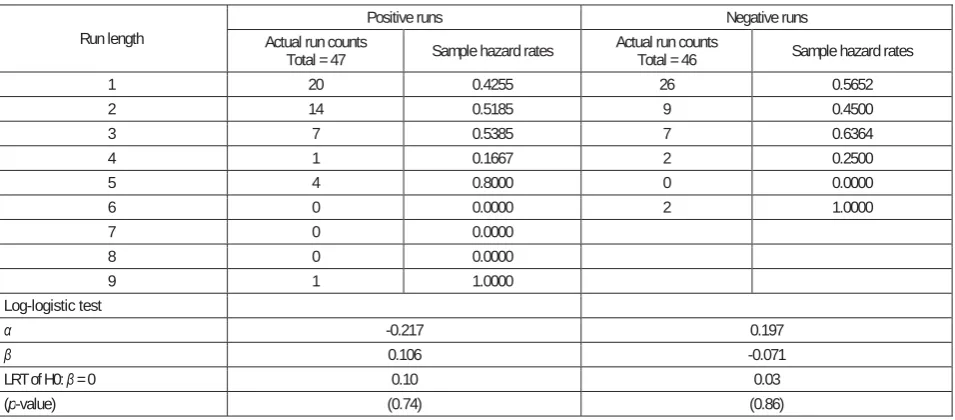
Table 1. Duration dependence test with log-logistic model for runs of monthly excess equally-weighted portfolio returns for the full sample period (June 1993-December 2008)

Run length

Positive runs Negative runs

Actual run counts

Total = 47 Sample hazard rates Actual run counts Total = 46 Sample hazard rates

1 20 0.4255 26 0.5652

2 14 0.5185 9 0.4500

3 7 0.5385 7 0.6364

4 1 0.1667 2 0.2500

5 4 0.8000 0 0.0000

6 0 0.0000 2 1.0000

7 0 0.0000

8 0 0.0000

9 1 1.0000

Log-logistic test

Į -0.217 0.197

ȕ 0.106 -0.071

LRT of H0: ȕ = 0 0.10 0.03

(p-value) (0.74) (0.86)

Notes: A run of length i is a sequence of i abnormal returns of the same sign. Positive and negative excess returns are defined rela-tive to the residual from the regression of real returns on its first three lags, the term spread, and the dividend yield. The sample hazard rate, hi= Ni / (Mi + Ni) represents the conditional probability that a run ends at i, given that it lasts until i, where Ni is the

count of is runs of length i and Mi is the count of runs with a length greater than i. The log-logistic function is hi = 1 / 1 + e-(Į + ȕLni). ȕ

is the hazard rate which is estimated using the logit regression where independent variable is the log of current length of the run and dependent variable is 1 if the run ends and 0 if it does not end in the next period. The LRT (likelihood ratio test) of the null hypothe-sis, H1: ȕ = 0, of no duration dependence (constant hazard rate) follows the Ȥ²(1) distribution. P-value is the marginal significance level, which is the probability of obtaining that value of the LRT or higher under the null hypothesis.

Table 2. Duration dependence test with log-logistic model for runs of monthly excess value-weighted portfolio returns for the full sample period (June 1993-December 2008)

Run length

Actual run counts

1 19 0.4318 22 0.5000

2 11 0.4400 13 0.5909

3 7 0.5000 5 0.5556

4 2 0.2857 2 0.5000

5 1 0.2000 1 0.5000

6 1 0.2500 1 1.0000

7 0 0.0000

8 3 1.0000

Log-logistic test

Į -0.239 0.025

ȕ -0.132 0.281

LRT of H0: ȕ = 0 0.20 0.43

(p-value) (0.66) (0.51)

Notes: A run of length i is a sequence of i abnormal returns of the same sign. Positive and negative excess returns are defined rela-tive to the residual from the regression of real returns on its first three lags, the term spread, and the dividend yield. The sample hazard rate, hi= Ni / (Mi + Ni) represents the conditional probability that a run ends at i, given that it lasts until i, where Ni is the

count of runs of length i and Mi is the count of runs with a length greater than i. 4. The log-logistic function is hi = 1 / 1 + e

-(Į + ȕLni) .

(7)

Table 3 reports the results of duration dependence test with log-logistic model for runs of monthly excess returns for the two sub periods. The results convey similar information to those of the full sample pe-riod. During the pre- and post-1997 Asian crisis, both equally- and value-weighted portfolio yield positive ȕ coefficients (0.765, 0.208, 0.278, 0.092) in positive runs. In negative runs, the equally-weighted portfolio yields negative ȕ coefficient

during pre-1997 crisis period (ȕ = -0.103) and posi-tive ȕ coefficient during post 1997 crisis period (ȕ = 0.174). The value-weighted portfolio yields posi-tive ȕ coefficient during pre-1997 crisis period (ȕ = 1.785) and negativeȕ coefficient during post 1997 crisis period (-0.024). However, both negative ȕ coefficients are not significant. Thus, the results for the two sub periods fail to reject the hypothe-sis of no bubble.

Table 3. Duration dependence test with log-logistic model for runs of monthly excess returns of both portfolios for sub periods

Į ȕ LRT (p-value) Į ȕ LRT (p-value)

Equally-weighted portfolio

Pre-1997 0.288 0.765 _(0.46)0.54 0.053 -0.103 _(0.87)0.03

Post 1997 -0.498 0.208 _(0.57)0.33 0.231 0.174 0.09 _(0.76)

Value-weighted portfolio

Pre-1997 0.492 0.278 _(0.77)0.08 -0.178 1.785 _(0.11)2.59

Post 1997 -0.691 0.092 _(0.79)0.07 0.050 -0.024 0.002 _(0.96)

Note: The likelihood ratio test follows the Ȥ²(1) distribution. The p-values are given in the brackets.

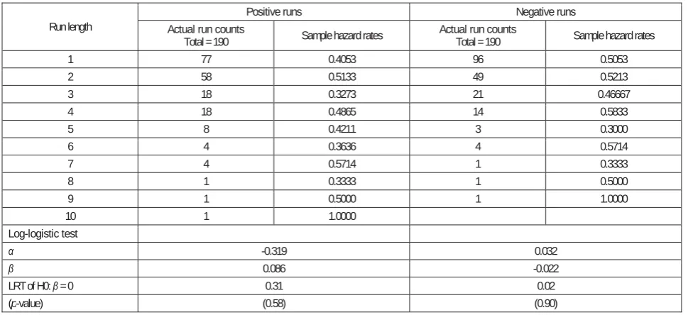
Tables 4 and 5 report the duration dependence test for the log-logistic model for runs of weekly excess equal-ly weighted and weekequal-ly excess value weighted port-folio returns for the full sample period (June 1993 to December 2008), respectively. For the equally-weighted portfolio, neither an increase nor decrease in the hazard rate pattern in positive runs is observed. This means that the probability of the run ending is independent of the prior sequence. The hazard rate

exhibits a relatively constant negative runs pattern (see Table 4). Similar hazard rate patterns are also observed in the value-weighted portfolio. These patterns are inconsistent with rational speculative bubbles (see Table 5). In addition, for the equally-weighted port-folio, the positive runs have a positive ȕ coefficient (ȕ = 0.086). Similar findings are also reported for the value-weighted portfolio (ȕ = 0.082). The results imp-ly no evidence of rational speculative bubbles. Table 4. Duration dependence test with log-logistic model for runs of weekly excess equally-weighted

port-folio returns for the full sample period (June 1993-December 2008)

Run length

Actual run counts

1 77 0.4053 96 0.5053 2 58 0.5133 49 0.5213

3 18 0.3273 21 0.46667

4 18 0.4865 14 0.5833

5 8 0.4211 3 0.3000

6 4 0.3636 4 0.5714

7 4 0.5714 1 0.3333

8 1 0.3333 1 0.5000

9 1 0.5000 1 1.0000

10 1 1.0000

Log-logistic test

Į -0.319 0.032

ȕ 0.086 -0.022

LRT of H0: ȕ = 0 0.31 0.02

(p-value) (0.58) (0.90)

Notes: A run of length i is a sequence of i abnormal returns of the same sign. Positive and negative excess returns are defined relative to the residual of the AR(4) model. The sample hazard rate, hi= Ni / (Mi + Ni) represents the conditional probability that a run ends at i,

given that it lasts until i, where Ni is the count of runs of length i and Mi is the count of runs with a length greater than i. The log-logistic

function is hi = 1 / 1 + e-(Į + ȕLni). ȕ is the hazard rate which is estimated using the logit regression where independent variable is the log of

(8)

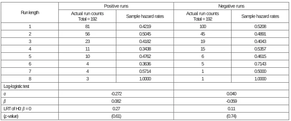
Table 5. Duration dependence test with log-logistic model for runs of weekly excess value-weighted portfolio returns for the full sample period (June 1993-December 2008)

Run length

Actual run counts

1 81 0.4219 100 0.5208

2 56 0.5045 45 0.4891 3 23 0.4182 19 0.4043 4 11 0.3438 15 0.5357

5 10 0.4762 6 0.4615

6 4 0.3636 5 0.7143

7 4 0.5714 1 0.5000

8 3 1.0000 1 1.0000

Log-logistic test

Į -0.272 0.040

ȕ 0.082 -0.059

LRT of H0: ȕ = 0 0.27 0.11

(p-value) (0.61) (0.74)

Notes: A run of length i is a sequence of i abnormal returns of the same sign. Positive and negative excess returns are defined rela-tive to the residual of the AR(4) model. The sample hazard rate, hi= Ni / (Mi + Ni) represents the conditional probability that a run

ends at i, given that it lasts until i, where Niis the count of runs of length i and Mi is the count of runs with a length greater than i.

The log-logistic function is hi = 1 / 1 + e-(Į + ȕLni). ȕ is the hazard rate which is estimated using the logit regression where independent

variable is the log of current length of the run and dependent variable is 1 if the run ends and 0 if it does not end in the next period. The LRT (likelihood ratio test) of the null hypothesis, H1: ȕ = 0, of no duration dependence (constant hazard rate) follows the Ȥ²(1) distribution. P-value is the marginal significance level, which is the probability of obtaining that value of the LRT or higher under the null hypothesis.

Table 6 reports the results of the duration depen-dence test on the two sub periods using the log-logistic model for runs of weekly excess returns. There is one negative ȕ coefficient observed in posi-tive runs, which occurs in the pre-1997 crisis period for the equally-weighted portfolio (ȕ = -0.064). But the negative ȕ is not significantly different from zero. In addition, the post-1997 period exhibits posi-tive ȕ coefficients. Thus, the findings in the two sub periods suggest that the null hypothesis of no duration dependence or constant hazard rate can-not be rejected.

We also test if bubbles exist between 1999-2001 and 2007-2008 using weekly data. Table 6 shows nega-tive ȕ coefficients (-0.321 & - 0.233) for both equal-ly-weighted and value-weighted positive runs for the period of 1999-2001. However, the weekly re-sults still fail to reject the no rational bubble hypo-thesis (p-values = 0.30 & 0.53). The equally-weighted portfolio returns yield negative ȕ (-0.127) but with an insufficient evidence (p-value = 0.77) for 2007-2008. On the other hand, the value-weighted portfolio returns yield positive ȕ, which also does not support the existence of rational bubbles. Table 6. Duration dependence test with log-logistic model for runs of weekly excess returns

of both portfolios for pre- and post-1997 Asian crisis

Į ȕ LRT (p-value) Į ȕ LRT (p-value)

Pre-1997 -0.032 -0.064 _(0.83)0.05 -0.139 0.174 _(0.60)0.28

Post-1997 -0.410 0.126 _(0.49)0.48 0.106 -0.103 _(0.63)0.23

1999-2001 -0.202 -0.321 1.07 _(0.30) 0.142 0.599 1.09 _(0.30)

2007-2008 -0.177 -0.127 _(0.77)0.08 0.271 -0.718 _(0.09)2.90

Pre-1997 -0.377 0.089 _(0.76)0.10 -0.039 -0.148 _(0.63)0.23

Post-1997 -0.233 0.086 0.20 _(0.65) 0.065 0.005 0.00 _(0.98)

1999-2001 0.100 -0.233 _(0.53)0.39 0.248 -0.291 _(0.47)0.51

2007-2008 -0.361 0.479 _(0.35)0.89 -0.337 0.265 _(0.59)0.29

(9)

3.1.2. Weibull hazard model. Table 7 shows the results for the Weibull hazard model for runs of monthly excess returns of the two portfolios. For the equally-weighted portfolio, the ȕ coefficients are positive but not significantly different from zero in

positive runs, which means the null hypothesis is not rejected. In addition, the value-weighted portfo-lio also does not reject the null hypothesis of ȕ = 0 in the full sample periods, as well as pre- and post-1997 crisis period.

Table 7. Duration dependence test (Weibull hazard model for runs of monthly excess returns for both portfolios)

Į ȕ _(p-value)LRT Į ȕ _(p-value)LRT

Full sample

period 0.424 0.054 (0.75) 0.10 0.570 -0.035 (0.85) 0.03

Pre-1997 0.391 0.399 _(0.38)0.78 0.545 -0.057 _(0.87)0.03

Post-1997 0.341 0.114 _(0.58)0.31 0.512 0.084 _(0.74)0.11

Full sample

period 0.478 -0.077 (0.66) 0.20 0.473 0.069 (0.51) 0.43

Pre-1997 0.560 0.105 _(0.76)0.09 0.321 0.55 _(0.06)3.59

Post-1997 0.315 0.060 _(0.79)0.07 0.519 -0.013 _(0.96)0.003

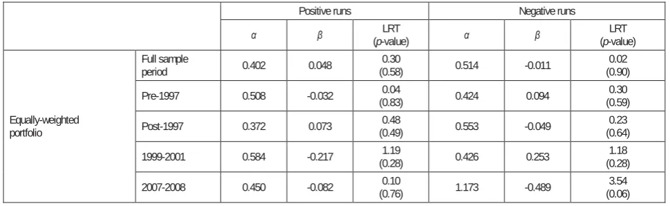
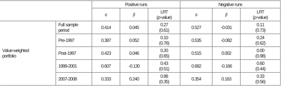
Table 8 reports the results of the duration depen-dence test using the Weibull hazard model for runs of weekly excess returns of the two portfo-lios. The results for weekly returns convey similar information as the monthly results. For the equal-ly-weighted portfolio, the estimated ȕ coefficient is positive (0.048) in positive runs, and negative (-0.011) in negative runs in full sample period. In sub periods, the ȕ coefficient is negative (-0.032) in positive runs and positive (0.094) in negative runs in pre-1997 period. The ȕ coefficient is also positive (0.073) in positive runs and negative (-0.049) in negative runs in post-1997 period. How-ever, all the ȕ coefficients are not different from zero regardless of whether the ȕ coefficients are positive or negative. For the value-weighted portfo-lio, the ȕ coefficients are positive in positive runs

(0.045, 0.052, 0.046) in the full sample period as well as in the sub periods. Negative coefficients (-0.031, -0.082) are obtained in negative runs of returns in full sample period and pre-1997 period, and post period coefficient is close to zero (0.002). Similar to the log-logistic model, Table 8 also shows the results of the bubble tests during 1999-2001 and 2007-2008 using the Weibull hazard mod-el with weekly data. Both equally- and value-weighted positive returns yield negative ȕ coeffi-cients (-0.217 & -0.130) for the period of 1999-2001, but the result is insignificant (p-values = 0.28 & 0.51). The equally-weighted positive returns yield negative ȕ (ȕ = -0.082; p-value = 0.76), for 2007-2008 is insignificant. The value-weighted positive returns yield positive ȕ (0.240). Therefore, the re-sults contradict the rational bubble hypothesis.

Table 8. Duration dependence test (Weibull hazard model for runs of weekly excess returns for both portfolios)

Full sample

period 0.402 0.048 (0.58) 0.30 0.514 -0.011 (0.90) 0.02

Pre-1997 0.508 -0.032 _(0.83)0.04 0.424 0.094 _(0.59)0.30

Post-1997 0.372 0.073 _(0.49)0.48 0.553 -0.049 _(0.64)0.23

1999-2001 0.584 -0.217 _(0.28)1.19 0.426 0.253 _(0.28)1.18

(10)

Table 8 (cont.). Duration dependence test (Weibull hazard model for runs of weekly excess returns for both portfolios)

Full sample

period 0.414 0.045 (0.61) 0.27 0.527 -0.031 (0.73) 0.11

Pre-1997 0.387 0.052 _(0.76)0.10 0.535 -0.082 _(0.62)0.24

Post-1997 0.423 0.046 _(0.65)0.20 0.515 0.002 _(0.98)0.00

1999-2001 0.607 -0.130 0.43

(0.51) 0.682 -0.166

0.60 (0.44)

2007-2008 0.333 0.240 _(0.35)0.88 0.354 0.163 _(0.56)0.33

The sensitivity analysis between the log-logistic model and Weibull hazard model for the same test-ing period and return portfolio showed the ȕ coef-ficients (positive or negative ȕ) are similar. In addition, there is no distinct difference between the results using monthly data and weekly data on both models. Furthermore, the results of positive or negative ȕ coefficients between equally-weighted and value-equally-weighted portfolios are slightly different in some area for the same model and same data series, but all ȕ coefficients are close to zero and statistically insignificant. There-fore the results of the duration dependence test in our study are not sensitive to the use of different models and data series. Though McQueen and Thorley (1994) state that equally-weighted portfo-lio results are more robust than value-weighted portfolio results in their study of the US stock markets, we find no evidence of this in the Hong Kong stock market because of the relatively high marginal significance level (p-value) for all the likelihood ratio tests, which are similar to the p- value in the likelihood ratio test in Yu and Sze (2003)’s study.

Conclusions

The results of the duration dependence tests did not show any evidence to support the existence of ra-tional speculative bubbles in the Hong Kong stock market, and the results do not differ between differ-ent hazard models, return weighting schemes and data frequency. The duration dependence test results of our study are similar with Chan at al. (1998) but contradict Yu and Sze (2003) who employed speci-fication and co-integration tests. Yu and Sze’s co-

integration test relies on expectations of future steams of dividends, utilizes linear rational expecta-tion model of stock price and assumes that the ex-pected real return of stock equals a constant re-quired real rate of return, but does not account for volatility of stock prices (Leroy and Porter, 1981; Shiller, 1981). Similarly, the problem of specifi-cation test arises from observing rational bubbles separately from the market fundamentals of the asset price (Diba, 1985). Thus, the duration de-pendence test is considered more reliable in obtain-ing robust results.

(11)

Fig. 2. Hang Seng Price Index (daily)

This implies that even when bubbles exist in the Hong Kong stock market the bursts are relatively slow, which is uncharacteristic of rational specula-tive bubbles. In fact, Chan at el. (1998) conduct an anecdotal test for the suspected bubble period in the Hong Kong stock market. The anecdotal evidence indicates increasing and explosive returns that is consistent with bubbles, but not the instantaneous crash as required by the rational bubble theory. Second, besides the rational speculative bubble model, there are broader concepts of bubbles includ-ing the fads model proposed by Summers (1986), manias and panics by Kindleberger (1989) and ran-dom speculative bubble by Weil (1987). It is possi-ble that the Hong Kong stock market is characte-rized by other types of bubbles other than rational speculative bubbles.

The results of this study provide some policy impli-cations. There are two possible explanations for higher stock prices – the reflection of improved “fundamentals” or the reflection of irrational beha-vior of investors about the firms’ prospect, which is one of the possible sources of non-fundamental movements in asset price (Bernanke and Gertler, 1999; Kroszner, 2003). Bernanke and Gertler (1999) point out that it is important to distinguish between fundamental and non-fundamental fluctuation in asset prices. This study shows that there is no empir-ical evidence of the existence of rational speculative bubbles in the Hong Kong stock market from 1993 to 2008. The result implies that the stock prices could most likely be a reflection of fundamentals.

For example in 1993, the increase in equity prices in Hong Kong was a reflection of the rapid growth of Mainland China and the listing of H-share compa-nies which started in 1993 (see Figure 2). During the period of 1995-1997, the stock market became bul-lish, reflecting improved business confidence as unemployment rate was at a low 2.1% and investors eased their worries of political uncertainty. The stock market was bullish again over technology issues during 1998-2000 as the GEM was intro-duced in 1999 to raise capital (Invested.hk, 2010) In the context of policy controlling market funda-mentals on the protection of market efficiency, there are several issues that the policy makers should address. Bernanke and Gertler (1999) suggest that the best policy framework to achieve price and fi-nancial stability is maintaining flexible inflation. Thus, this target induces policy makers to adjust interest rates to offset incipient inflationary or defla-tionary pressure. To reduce share price bubbles, interest rates should be raised when asset prices rise and reduced when asset prices fall (Bernanke and Gertler, 1999; Mokhtar et al., 2006). Kroszner (2003) also argue that enhancing the transparency of the equity market would make the information easi-ly accessible to investors that are able to reduce information asymmetry to prevent bubbles. In addi-tion, the development of financial infrastructure such as the payment systems and constructing de-rivative products based on price jumps may help hedge the political risk (Kim and Mei, 2001; Yu and Sze, 2003).

References

1. Abdul-Haque, Wang, S. & Oyang, H. (2008). “Rational Speculative Bubbles in Chinese Stock Market”, Interna-tional Journal of Applied Economics, 5 (1), pp. 85-100.

2. Ali, N., Nassir, A., Hassan, T. & Abidin, S.Z. (2009). “Stock Overreaction and Financial Bubbles: Evidence from Malaysia”, Journal of Money, Investment and Banking, 11, pp. 90-101.

(12)

4. Bernanke, B. & Gertler, M. (1999). “Monetary Policy and Asset Price Volatility”,Paper presented at the Federal Reserve Bank of Kansas City conference on “New Challenges for Monetary Policy”, Jackson Hole, Wyoming, August 26-28.

5. Blanchard, O.J. & Watson, M.W. (1982). “Bubbles, Rational Expectations and Financial Markets”, NBER Work-ing Paper Series 945, pp. 1-30.

6. Chan, K., McQueen, G. & Thorley, S. (1998). “Are there Rational Speculative Bubbles in Asian Stock Market?”,

Pacific-Basin Finance Journal, 6, pp. 125-151.

7. Das, A. (2007). “Testing a Hazard Model for the Housing Market in New Orleans”, American Journal of Econom-ics and Sociology, 66(2), pp. 443-455.

8. Diba, B.T. & Grossman, H.I (1985). “The Impossibility of Rational Bubbles”, NBER Working Paper No. 1615, Revised December.

9. Fama, E.F. & French, K.R. (1993). “Common Risk Factors in the Returns on Stocks and Bonds”, Journal of Fi-nancial Economics, 33, pp. 3-56.

10. Haque, A., Wang, S., & Oyang, H. (2008). “Rational Speculative Bubbles in Chinese Stock Market”, International Journal of Applied Economics,5(1), pp. 85-100.

11. Harman, Y.S. & Zuehlke, T.W. (2004). “Duration Dependence Testing for Speculative Bubbles”, Journal of Eco-nomics and Finance,28, pp. 147-55.

12. Invested.hk. (2010). Retrieved from http://bestanalytic.com/invested.hk].

13. Jaradat, M.A. (2009). “An Empirical Investigation of Rational Speculative Bubbles in the Jordanian Stock Market: A Nonparametric Approach”, International Management Review, 5 (2), pp. 92-97.

14. Jirasakuldech, B., Campbell, R.D. & Knight, J.R. (2006). “Are there Rational Speculative Bubbles in REITs?”,

Journal of Real Estate Finance and Economics, 32, pp. 105-127.

15. Jirasakuldech, B., Emekter, R. & Rao, R. (2007). “Do Thai stock Prices Deviate from Fundamental Values?”,

Pacific-Basin Finance Journal, 16, pp. 298-315.

16. Kim, H.Y. & Mei, J.P. (2001). “What Makes the Stock Market Jump? An Analysis of Political Risk on Hong Kong Stock Returns”, Journal of International Money and Finance,20, pp. 1003-1016.

17. Kindleberger, C.P. (1989). “Manias, Panics and Crashes: A History of Financial Crises”, Macmillan, London. 18. Kroszner, R.S. (2003). “Asset Price Bubbles, Information, and Public Policy. In Hunter, C., Kaufman, G. and

Pomerleano, M. (Eds) (2003). Asset Price Bubbles: The Implications for Monetary, Regulatory and International Policies, Cambridge, MA: MIT Press, pp. 3-12.

19. Lavin, A.M. & Zorn, T.S. (2001). “Empirical Tests of the Fundamental-Value Hypothesis”, Journal of Real Estate Finance and Economics, 22, pp. 99-116.

20. Lehkonen, H. (2010). “Bubbles in China”, International Review of Financial Analysis, 19, pp. 113-117.

21. LeRoy, S.F. & Porter, R.D. (1981). “The Present-Value Relation: Tests Based on Implied-Variance Bounds”,

Econometrica,49, pp. 555-574.

22. McDonald, J.B., McQueen, G. & Thorley, S. (1995). “Testing for Duration Dependence with Discrete Data”, Working Paper, Brigham Young University, Provo, UT.

23. McQueen, G. & Thorley, S. (1994). “Bubbles, Sock Returns and Duration Dependence”, Journal of Financial an Qualitative Analysis, 29, pp. 196-197.

24. Mokhtar, S.H., Md. Nassir, A. and Hassan, T. (2006). “Detecting Rational Speculative Bubbles in the Malaysian Stock Market”, International Research Journal of Finance and Economics, 6, pp. 102-150.

25. Rangel, G. & Pillay, S.S. (2007). “Evidence of Bubbles in the Singaporean Stock Market”, Singapore Economic Review Conference.

26. Shiller, R.J. (1981). “Do Stock Prices Move too Much to be Justified by Subsequent Changes in Dividends?”,

American Economic Review, 71, pp. 421-436.

27. Sichel, D.E. (1991). “Business Cycle Duration Dependence: A Parametric Approach”, Review of Economics and Statistics, 73, pp. 254-260.

28. Summers, L.H. (1986). “Stock Prices and Social Dynamics”, Brooking Papers on Economic Activity, 2, pp. 457-510. 29. Watanapalachaikul, S. & Islam, S.M.N. (2007). “Rational Speculative Bubbles in the Thai Stock Market:

Econo-metric Tests and Implications”, Review of Pacific Basin Financial Markets and Policies,10 (1), pp. 1-13.

30. Weil, P. (1987). “Confidence and the Real Value of Money in Overlapping Generation Models”, Quarterly Jour-nal of Economics, 102 (1), pp. 1-22.

31. Wu, G. & Xiao, Z. (2008). “Are there Speculative Bubbles in Stock Markets? Evidence from an Alternative Spproach”, Statistics and Interface, 1, pp. 307-320.

32. West, K.D. (1987). “A Specification Test of Speculative Bubbles”, Quarterly Journal of Economics, 102, pp. 553-580. 33. Yu, I. & Sze, A. (2003). “Testing for Bubbles in the Hong Kong Stock Market”, Hong Kong Monetary Authority

Working Paper, April.

34. Zhang, B. (2008). “Duration Dependence Test for Rational Bubbles in the Chinese Stock Market”, Applied Eco-nomics Letters, 15 (8), pp. 635-639.