Review
On to the next chapter for crop breeding: Convergence
with data science
Elhan S. Ersoz1,2,∗ , Nicolas F. Martin2 , and Ann E. Stapleton3
1 Umbrella Genetics, 2501 Woodridge Road, Champaign, IL 61822; [email protected] 2 Department of Crop Sciences, University of Illinois, Urbana-Champaign, 61820; [email protected] 3 Department of Biology and Marine Biology, University of North Carolina Wilmington,601 S. College,
Wilmington, NC 28401; [email protected]
* Correspondence: [email protected]; Tel.: +1-515-346-2259
Version March 6, 2019 submitted to Crop Science
Abstract: Crop breeding is as ancient as the invention of cultivation. In essence, 1
the objective of crop breeding is to improve plant fitness under human cultivation 2
conditions, making crops more productive while maintaining consistency in life cycle 3
and quality. The applications of predictive breeding has been gaining momentum in 4
agricultural industry and public breeding programs for the last decade, in the aftermath 5
of genomic selection being recognized and widely applied for accelerating genetic gain 6
in breeding programs. The massive amounts of data that has been generated by industry 7
and farmers year after year through several decades has finally been recognized as an 8
asset. A wide range of analytical methods such as machine learning, deep learning and 9
artificial intelligence that were initially developed for diverse quantitative disciplines are 10
now being adopted to crop breeding decision making processes. New technologies are 11
currently being developed that would enable integration of data from various domains 12
such as geospatial variables and a multitude of phenotypic responses as well as genetic 13
information, in order to identify, develop and improve crop faster via partial or full 14
automation of the decisions that pertain to variety development. Here we will discuss 15
and summarize efforts from public and private domains for predictive analytics, and 16
its applications to crop breeding and agricultural product development, and provide 17
suggestions for future research. 18
Keywords: machine learning; agroclimactic modelling; crop breeding and genetics; 19
GxE 20
Abbreviations
21
The following abbreviations are used in this manuscript:
22 23
Submitted toCrop Science, pages 1 – 28 www.mdpi.com/journal/crscj
ML Machine Learning DL Deep Learning AI Artificial Intelligence GS Genomic Selection
GEBV Genomic Estimated Breeding Value GWAS Genome-wide Association Study MET Multi-environment trials
TPE Target Population of Environments QTL Quantitative Trait Locus
MAS Marker Assisted Selection
MARS Marker Assisted recurrent Selection MAB Marker Assisted Backcross Introgression GM Genetically Modified
GxE Genetics-by-Environment interactions MLM Mixed-Linear Model
AMMI Additive Main effects and Multiplicative Interaction Model RM Relative Maturity
CNN Convolutional Neural Networks RNN Recurrent Neural Networks
24
1. Introduction: How did we get here?
25
Although the common wisdom states that the only objective of crop breeding is 26
to improve productivity, i.e. yield – this is clearly an oversimplification. The actual 27
root objective of breeding is to improve cultivate-ability, while increasing productivity 28
(Borlaug,2007). 29
Cropping systems vary widely- and are conditional on the available resources and 30
constraints at the time of cultivation. Some of the general features that define the 31
cultivation conditions are geography and climate of the farm; economic, social and 32
political pressures; available technologies and instruments as well as the philosophy and 33
culture of the farmer and the society (Borlaug,2007). All these constraining features of 34
cultivation are very temporally dynamic, with the exception of geography and climate. 35
Geography and climate are the only features of cropping systems that are stable over 36
time and thus are long-term influencers of crop improvement practices through-out the 37
ages (Bullock,1992). 38
Crop improvement practices in reality, require a breeder to address multiples of 39
breeding goals some of which are antagonistic (Kwon and Torrie,1964;Meredith and 40
Bridge,1971;Kato and Takeda,1996;Triboiet al.,2006;Erskineet al.,1985). These goals 41
are frequently related to productivity and cropping systems, as well as post-harvest 42
characteristics and cost-of-goods and economics of seed production systems (Guanming 43
between protein and oil content of the seed that is postulated to be rooted in C-N 45
partitioning biochemistry and physiology of the seed(Reekie and Bazzaz,1987;Moose 46
et al.,2004;Guoet al.,2013;Liet al.,2010). Likewise, negative correlations were reported 47
for traits like fruit size and number of inflorescences in various plants(Reekie and Bazzaz, 48
1987;Schoen and Dubuc,1990), or between overall seed yield and protein content in 49
some crops such as wheat and soybeans (Oury and Godin,2007;Rotundoet al.,2009) 50
and between plant biomass and seed yield in grasses like sorghum (Piper and Kulakow, 51
1994). 52
Crop-wildrelatives studies comparing the degree of antagonism between these 53
correlated traits for elite and native versions of crop species revealed that the extreme 54
antagonisms observed in elite crop varieties are often variety specific, and are likely to 55
be driven by the genotype x environment x cropping systems interactions and genetic 56
drift- due to the bottlenecks the breeding populations experience under extreme selection 57
(Ledford,2017;Greeneet al.,2018;von Wettberget al.,2018), a concept referred to as 58
genetic erosion (Van de Wouwet al.,2010). 59
Modern studies with mutants and gene editing successfully validated that these 60
antagonisms are often undesirable by-products of domestication and breeding practices 61
(Ledford,2017), and indeed some can be overcome by genetic modifications (Li et al., 62
2015;Soyket al.,2017) albeit at the cost of adding an additional trait to select into the 63
breeders’ tally of breeding goals. 64
These and other constraints described previously lead to breeding selections and 65
advancement decisions in a breeding program becoming a complicated balancing act; 66
approaches for balancing the various priorities are still heavily debated(Batista et al., 67
2018). Some favor straight truncation selection, others suggest applying index selection, 68
with variable indices at each advancement stage gates, with no consensus over a standard 69
process. 70
The changing economics of the seed industry starting around the late 1980’s set 71
the breeders up for yet another incredibly hard task: Starting with the existing elite 72
varieties-those that are indeed regionally adapted and genetically differentiated, create 73
varieties that are adapted to large cropping areas that demonstrate stable performance 74
across environments 1 Following the development of the transformed strain, the
75
transgene is then conventionally back-cross introgressed into the rest of the elite 76
germplasm. 77
Since this is a costly process, economic and practical constraints have driven the 78
number of varieties that should be designated elite for marketing to a fraction of what it 79
1 This objective was driven by the emergence of GM technologies. In most crops, there is only a single
was before. Regional adaptation concept started to be frowned upon, and the quest for 80
finding that elusive elite line that works well everywhere began(van Eeuwijket al.,2016). 81
Since all the starting material was elite, and all had acceptable productivity traits, 82
the logical reasoning for how to achieve this task was through modification of flowering 83
time characteristics of an existing variety so that it could be grown in additional relative 84
maturity zones (Doubler,2016). The proposed path to doing so was through backcross 85
introgression and directional selection. The idea was if a cross between a high-line and 86
a low-line for the favorable trait is available then a cross between the two would be 87
segregating for the desirable trait. The breeder then could start back-crossing selected 88
progeny to either parent to create recombinant-lines that would only be different from 89
the target parent in its flowering time characteristics, but would otherwise be identical to 90
parental phenotypes. 91
Although the logic of this process- a natural extension to decades long QTL mapping 92
and marker assisted breeding studies- was correct and applicable to some crops, i.e. 93
soybeans (Doubler,2016), the complex nature of the flowering time as a trait in many 94
other crops, influenced by hundreds of QTL with numerous alleles was not amenable to 95
this approach(Buckleret al.,2009). The genetic architecture of flowering time is highly 96
complex in many crop species and thus involves multitudes of loci scattered across 97
the genome. An attempt to co-introgress more than a handful of donor loci alleles to 98
a recipient background with only limited number of recombination possibilities in a 99
biparental cross creates a requirement for hundreds of thousands of progeny per cross 100
to be generated at each back-cross generation to find the elusive recombinants with the 101
right combination of alleles across their genome. 102
One recent example that demonstrates this process clearly is the Tenallion (2018) 103
study, where the authors employed 13 generations of divergent selection to an initial 104
biparental cross, and obtained five distinct populations with a time-lag of roughly two 105
weeks between Early- and Late/VeryLate-flowering populations (Tenaillonet al.,2018). 106
Although this may attest to the feasibility of such a process, 13 generations roughly 107
translates to 6 years of breeding, minimum. Therefore, it is clearly not-optimal for 108
commercial product development, where a product life cycle for seed varieties are often 109
estimated to be at 6 to 7 years. 110
After about three decades of trying to full fill these objectives with a combination 111
of marker assisted breeding(Ribaut and Hoisington, 1998) and ideotype selection
112
approaches(Gauffreteau,2018) breeders finally realized that for majority of breeding 113
objectives (e.g. improve yield, change RM and introgress transgenes and disease 114
resistance alleles at the same time) this was a logistically challenging task and rarely 115
produced the fully intended product. The number of loci that required concurrent 116
Figure 1. Number of maize patents filed between 1987 and 2017, ordered by their priority dates, and broken down as inbred( gold) and hybrid(blue). Data extracted from patents.google.com, and is available as supplementary material. The number of inbred lines developed is more uniform over time, while the number of hybrids show a big jump, starting in 2007, marking the onset of priority shifts from inbred line development to hybrid testing driven by hopes of generating hybrids of existing elite parents that can work over larger geographies. The dip observed in hybrid numbers in 2015 marks the onset of the products developed through predictive modelling, whereby cutting back the numbers for expensive advanced stage testing,trialing and registration.
desired properties increased. As a result, the process quickly became intractable with 118
existing methods, and far exceeded the desired delivery times and created undue stress 119
on logistics and operations (Tutino,2016). 120
Rate of genetic gain in breeding programs stayed stagnant, and ambitious product 121
development deadlines set due to increasing economic pressures in the competitive 122
markets passed unmet which in turn effected the economics of the organizations and 123
the research funds available for breeding. These trends are reflected in the number of 124
inbred and hybrid variety patents filed for maize and soybean varieties, comparing the 125
historical trends with those after 2010 (Figure1). These economic limits were one of the 126
significant drivers that lead to the adoption of genomic selection as a concept, and the 127
breeding community embracing predictive modelling as the method of choice for rapid 128
Genomic selection offers the unique perspective of selecting the best individuals out 130
of the available population pool, in contrast to trying to create the ideal individual based 131
on an ideotype, hence removing the constraint for selecting the best alleles at each loci in 132
a trade-off for selecting the best combination of alleles across the genome that work well 133
together and is already available within the set of existing varieties. 134
2. Scribes, Prophets and Match Makers: Clustering, Classification and
135
Combinatorics for Breeding
136
"Predictive algorithms start out as historians: they study historical data to detect 137
patterns. Then they become prophets: they devise mathematical formulas that explain 138
the pattern, test the formulas against historical data withheld for the purpose, and use 139
the formulas to make predictions about the future."Lepore(2018) 140
2.1. Prediction of Unobserved Phenotypes by their genomic similarity to known samples 141
One of the earliest and most widely used applications of machine learning in crop 142
breeding is its utilization for prediction of unobserved phenotypes, based on genetic 143
markers. This process often referred to as GEBV estimation (for Genomic Assisted 144
Breeding Value estimation) utilizes the resemblance between relatives principles as 145
measured by the genomic similarity between individuals in a population. The initial 146
applications leveraged pedigreed populations, where the parents of a bi-parental cross 147
and their progeny were used to develop models that could predict un-observed progeny 148
phenotypes from the same cross (Meuwissenet al.,2001;Meuwissen and Goddard,2001). 149
Later on, methods were developed to apply similar principles to predict phenotypes for 150
un-pedigreed, diverse line populations leveraging identical by state based resemblence 151
between individuals as opposed to identical by descent(Peiffer et al.,2014;Ersoz ES, 152
2017). 153
Statistically this is a very straightforward process, wherein the genome is 154
characterized by assayable markers, where the markers are assayed in both parents 155
and in a fraction of the progeny. In a sense, this step leverages the same principles as 156
QTL mapping approaches - where the objective is assignment of a phenotypic value 157
to each segment of the genome. The main operational difference from QTL-mapping 158
lies in the fractionation of phenotypic variation that is attributed to each marker. While 159
in QTL mapping this objective is achieved through a direct test of correlation between 160
the allelic state at a genomic position vs. the phenotype, in many GS applications 161
the first step is inference of individuals’ similarities to each other via calculation of a 162
G- matrix, and then fractionating the G-explained phenotype. The more conceptual, 163
theoretic distinction between QTL mapping and GS is in how the genetic differences 164
are modeled to contribute to the phenotype, with the QTL models primarily targeting 165
small-effects as a composite value across all intervals in the genome (Meuwissen and 167
Goddard,2001). More recent models allow searching and reporting both types of effects 168
and use flexible distributions (Moseret al.,2015). 169
Naturally, this approach was first applied to fully characterized populations where 170
predicted and observed phenotypic values have been compared and contrasted. The 171
level of correlation between the observed versus expected phenotypes define the level 172
ofaccuracy-of-predictionthat can be achieved by this approach. Since 2010, the research 173
community has focused on ways to incorporate flexibility and additional features into 174
these models, including environmental parameters, as well as genotype-environment 175
interaction (g x e) terms. 176
Nonlinear components can also be added into the linear predictions (Voss-Felset al., 177
2018). Nonlinear (epistatic or conditional) predictions are especially important in elite 178
breeding populations; the form of g x e selection will vary between optimization for 179
wide adaption varieties and specific small-holder or regionally-branded varieties – but 180
consideration of the environment is now an integral part of genomic selection algorithms 181
(Voss-Felset al.,2018). 182
2.2. Paradox of Choice: Many methods one GEBV 183
There are many recent published examples of selection on relatively small scale 184
data sets in crop and animal breeding (Gorjancet al.,2018;Dimitrijevic and Horn,2018; 185
Ozimatiet al.,2019;Rioet al.,2019;Sweeneyet al.,2019). Linear methods such as GBLUP 186
typically work quite well for building predictions for almost all applications. Heslot 187
et al.(Heslot et al., 2012) compared and contrasted performance metrics from several 188
methods (Heslot et al., 2012) and concluded that when multiple methods have been 189
applied to the same data set, prediction quality is often similar for GBLUP, bayesian 190
models, and recursive partitioning methods such as random forest (Heslotet al.,2012) – 191
however the exact set of SNP alleles varies with the specific method. These comparisons 192
reported were based on predictions in biparental populations. 193
When various methods and models were compared for their predictive accuracy in 194
un-pedigreed populations, however, the observation was that optimization of the training 195
population composition based on relatedness to a target population can potentially 196
increase the prediction accuracy and alter the algorithmic efficacy of various methods 197
and models applied for within and cross-population for prediction accuracies and GEBV 198
calculations (Ersoz ES,2017). 199
Multi-environment studies for variety testing and development are often statistically 200
under powered for detecting small effect sizes, due to the economic trade-off created 201
by the total number of plots that can be included in an experiment. Breeders are often 202
required to choose between small number of samples in many sites vs. large number of 203
power studies to guide such choices, these decisions are often driven by operational 205
optimization concerns based on advancement stage of the material tested. In early stages 206
of line development, few sites with many samples are favored, while in later stages many 207
sites with few samples are favored. 208
This logistic limitation of multienvironment testing, often disregards the variability 209
expected in QTL effects across environments by virtue of GxE, as well as penetrance, as 210
nuisance parameters2that are anticipated but are not expected to effect the estimates of 211
"real effectors". 212
Since the underlying objective in commercial breeding is oftenadaptation to large 213
geographies and cropping systems, only the effects that can be detected despite these 214
limitations are considered "real" and are leveraged for MAS applications. This process 215
inadvertently creates an implicit selection bias against GxE responsive QTL in elite 216
variety testing and material development. 217
Another concern in QTL mapping and genomic selection is perceived pleitrophy 218
3. As was described previously, both QTL mapping and GS approaches work through
219
fragmental evaluation of the genome for the correlated change in allele states and 220
the phenotype of interest. The larger the size of each fragment evaluated, the higher 221
the likelihood that it will contain QTL for more then one phenotype, especially if the 222
phenotypes of interest are complex in their genetic architecture (large number of small 223
effect QTLs). We are calling this phenomenonperceived pleitrophyas opposed to genetic 224
pleitrophy, since it is in fact an artifact of the analysis methods and does not actually 225
offer any insights into the molecular nature of co-regulation of multiple phenotypes. 226
Kemperet al.(2018) has shown with simulations that the assumption of pleitrophy 227
across multiple environments, generates significantly different results in contrast to 228
analysis of each trait-environment combination individually. The difference was often 229
not a significant change in predictive efficiency, but rather in the distribution of significant 230
effects and the markers implicated to capture that variation. 231
This and the observation that any random set of independent markers are as 232
predictive as known-allele/effector networks in explaining observed phenotypic 233
variation (Buckleret al.,2009) casts doubt over the utility of GS and by proxy GWAS in 234
its ability to identify functional variation (Mooreet al.,2018). More work is needed to 235
understand such observations as to their cause, whether they are artifacts of the methods 236
used, or if they are biologically based. 237
2 See Nuisance Parameterhttps://en.wikipedia.org/w/index.php?title=Nuisance_parameter&oldid=
875520938
Figure 2.Graph network of potential breeding crosses considered
2.3. Black sheep to Black Swans : Parent, Cross and Progeny Selection 238
The first practical question any breeder needs to repeatedly address at the beginning 239
of each and every breeding cycle is which crosses to make, or in other wordsparent & 240
cross selection. This problem is a variation of a very well studied mathematical problem, 241
formally known as combinatorics. It is defined as dealing with combinations of objects 242
belonging to a finite set in accordance with certain constraints. One of the oldest and 243
most accessible parts of combinatorics is graph theory and set theory. 244
Assume you have lines A1,A2,A3 and B1,B2,B3 available to make crosses with 245
Figure 2. You start with the constraint that the A types should not be crossed with 246
each other and neither does B types. Of the remaining nine combinations, you need to 247
pick one. An additional constraint is that you would like to maximize the transgressive 248
segregation potential of the cross, with generating the maximum number of progeny 249
that perform better than either parent. 250
This problem can be visualized as a network graph (Figure2). The graph consists 251
of six nodes and nine vertices and is not directed- meaning the direction of the vertices 252
from node to node is not defined. If the directionality of a cross is important for the 253
process (e.g. Although monoecious, the lines will be treated like they are diocious: A 254
lines will be designated females, andBlines will be designated males, and reciprocals 255
are not considered equal), the direction can also be defined. 256
Let’s assume that each of the vertices carry a weight. This weight can be the genetic 257
distance or similarity between the nodes (Figure 3a), the average yield observed in 258
the F1 when the two parents at the nodes were crossed (Figure3b), or the fraction of 259
transgressive segregants observed in the past experiments when these crosses were 260
made(Figure 3c), or a vector or scalar combination of all of the above weights. For 261
visualization purposes, the lengths of the vertices can be scaled to represent their weights, 262
which would present an immediate visual representation of all of the above mentioned 263
relationships between nine individual lines. 264
The intuitive visuals is just one advantage of using graph models to visualize 265
Figure 3.Example cross network graphs with the vertices scaled according to A. Genetic distance, B. average F1 yield, C.Fraction of transgressive segregants. If no transgressive segregation was observed, the vertex was deleted.
described allows applications of graph mining methods and kernel methods for ranking, 267
clustering and classification of nodes(parents) and vertices(crosses) in a graph model. 268
Furthermore, graph models allow for application of methods such as link analysis 269
(Harper and Harris,1975) and algorithms such as PageRank (Pageet al.,1999) that were 270
originally developed for Social Network analysis. These methods would provide new 271
methods for predicting the weight/value of an unobserved vertex(cross) from existing 272
cross networks (Park and Yook,2014) (Figure4A,4B), with or without leveraging genetic 273
marker information. 274
This type of analytics opens up extensive possibilities for breeders, and will also 275
allow integration of data across different experiments- that are partially overlapping 276
across time and geographies(Simko and Pechenick,2010). 277
Furthermore, these algorithmic applications allow development of learning-systems 278
Figure 4.A. Incomplete network graph representation of observed breeding crosses B. The complete network with the unobserved vertices shown as dashed lines, representing predictions
3. Introgression in Breeding : Applications of Mathematical Optimization &
280
Shortest Path Algorithms for machine learning
281
Marker assisted selection applications (MAS - MARS) have a long history in crop and 282
animal improvement (Ribaut and Hoisington,1998;Lande and Thompson,1990;Haley 283
and Visscher,1998;Ribaut and Ragot,2006). Despite the high hopes of the breeding 284
community to apply MARS for multiple traits simultaneously for multivariate index 285
selection, the method’s dependency on very large sample sizes to achieve sufficient 286
efficiency (Lande and Thompson,1990) have restricted its use and limited its success. 287
In fact, literature reports on theoretical efficiency of multi-trait MAS are scarce and 288
the theoretical limits of efficiency were not empirically tested and published until 2010 289
(Togashi and Lin,2010). Togashi and Lin examined the effectiveness of five different 290
selection methods under 72 scenarios. They reported that an index consisting of three 291
traits which are controlled by 40, 50 and 60 segregating loci, respectively, each with two 292
alleles would require 340 x 350x 360 =3.7 x 1071 different kinds of aggregate genotypes-293
which arguably can not all be available in the standing population under selection- and 294
led to the acknowledgement that MAS applications for low heritability, high complexity 295
phenotypes are practically not feasible. 296
The most important and historically most successful application of MAS in breeding 297
is for backcross-introgression of a single high value locus- such as a transgene, into 298
new genetic backgrounds, that is also known as MAB for Marker Assisted Backcrossing. 299
In MAB, the objective is to introgress the target region to a new genetic background 300
with the minimum amount of linkage drag(Hospital, 2005). The very first and most 301
material(Ragot et al.,1995). In MAB, foreground selection and background selection are 303
applied simultaneously controlling for the size of the introgression at the target as well as 304
other potential introgressions from the donor to the recipient by maximizing the recipient 305
allele recovery across the background, respectively at each generation of backcrossing. 306
For a review of early applications and successful examples of MAS and MAB see (Collard 307
and Mackill,2008) and the references therein. 308
The practical problems that needs to be addressed for improvement of preexisting 309
varieties is based on the idea of routinely generating rationally driven combinations of 310
functional genetic variants (Wallaceet al.,2018) in a target background. The task is the 311
same as it was defined in MAS several decades ago, however the scale and efficiency 312
needed to increase. In natural evolutionary processes, there are two complimentary 313
processes recognized for their efficacy in rapid creation of genetic novelties: hybridization 314
and introgression. In crop breeding however, due to its often unpredictable outcomes, 315
hybridization is often avoided, and introgression is preferred. 316
Here we suggest combining controlled hybridization with subsequent recurrent 317
selection to increase the speed and scale of the process, leveraging mathematical 318
optimization(Evans, 2017) and shortest path algorithms (Festa, 2019). Assume that 319
we are staring with a collection of 5 individual elite varieties, each of which posses 10 320
favorable haplotypes for a total of 50 loci to be combined in one background. Assume 321
that the ranking of each haplotype for each locus in the recipient background is also 322
available. The task is to maximize the individual locus haplotype ranks while minimizing 323
the number of crosses to be made and the number of progeny required per cross. 324
We would start with evaluating the pairwise genetic relatedness between the 325
recipient and the donors, which can be visualized as a network graph, where the nodes 326
are the individuals and the vertices are a measure of genetic relatedness between the 327
individuals. Each node has 10 unique alleles/loci to contribute, including the 10 that are 328
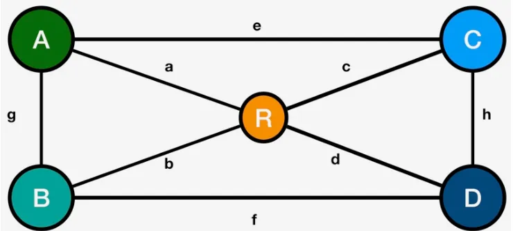
Figure 5.The graph model network of genetic relatedness between the donors and the recipient described in Section 3
To avoid the unpredictable outcomes of hybridization (non-linear responses), the 330
first step would be the identification of the closest pairs, which would maximize the 331
linear response outcomes in the hybrid. In this example, it will beg, the distance between 332
A−Bpair andh, the distance betweenC−Dpair. An ABF1 will have all the favorable 333
alleles from both A and B as heterozygotes in the cross. Similarly, a CDF1 will have 334
all the favorable alleles available. That is a total of two crosses. Now lets cross ABxR 335
andCDxR. Next we crossABRxCDRallowing all 50 alleles to segregate in the ABRCD 336
population. ABRCDpopulation will contain any number of combinations of alleles at
337
the 50 loci of interest would be equivalent to an F2 population, in relation to any one of 338
the parents. 339
We can then evaluate the available progeny for their allelic composition, and identify 340
a number of progeny to be back-crossed to the R parent. We continue backcrossing
341
hybrids to theRparent, until the introgression size at each of the 50 loci is reduced to 342
under 1 cM. In other words, the genome is allRminus 40 cM of introgressions. 343
Note that we have not yet made a selection based on ranks at each locus, just created 344
a diverse set of introgression lines, that can realize any number of possible combinations 345
of alleles across the 50 targets. Next, we rank each of the available progeny for their 346
predicted values across each of the loci, and pick the ones that scores the max. 347
That is 4-5 generations of crosses, for population development (two for hybridization, 348
2-3 for backcross introgression).The algorithm described above can easily be applied to 349
larger number of donors and larger number of loci. The time to complete hybridization 350
in number of generations will bex, where number of donors N =2x Number of back
351
crosses required will be proportional to the total size of the introgressions measured as 352
percentage of the genome. The larger the sum of all introgressions, shorter the number 353
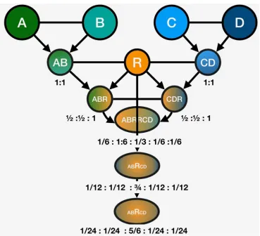
Figure 6. Each generation of crosses described in the scenario in section 3 of the manuscript. At the end of each generation, the expected genomic contribution of each parent is listed under the nodes. A total of 5 generations of crosses shown, at the end of which the expected value of genomic contribution ratio for each ofA,B,C,Deach are 1/24thwhileRis 5/6th. The variance around these expectation can be estimated by simulations
When a large collection of individuals(hundreds of thousands) in a breeding 355
population are considered, the path defined above to a fully stacked line, can be evaluated 356
by using algorithms such as gradient descent in neural networks. The algorithm will 357
need to go through iterative cycles of identifying crosses that carry favorable alleles to be 358
combined but are otherwise most similar to each other in overall genetic composition, 359
followed by GEBV calculations for the resulting progeny, and ranking of the progeny for 360
their potential to carry maximum number of favorable alleles going into a back-cross. It 361
will then evaluate every progeny generated as a result of the back-cross process for its 362
GEBV and provide rankings to be advanced to the next generation of back-crosses. 363
In simpler terms, this is an iterative decision process, where in each step, most closely 364
placed pair of lines are selected, and used for creation of cross, and the F1 of that cross 365
hybridization is achieved, and then the resulting lines are cleaned up and ranked for 367
most favorable combinations. 368
This approached was utilized in an unusual product development project by 369
Syngenta (Ritchie et al., 2017). Briefly, one of the coveted maize products developed 370
that carry an over-expressed transgene for Vip3A protein that was shown to confer 371
insecticidal effects resulting in chewing insect resistance with no negative impact on 372
the hybrid productivity phenotypes. However, later on it was revealed that Vip3A can 373
cause decreased male fertility in certain inbred maize plants under normal growing 374
conditions, creating issues around parent line maintenance, and hybrid seed production. 375
In a multi-year, multi-environment study, nine QTL across various locations across the 376
genome that create this male sterility phenotype has been identified. The research team 377
then utilized the hybridization:backcrossing approach described here to develop an 378
introgression plan for introgressing these QTL back into a large set of commercial line 379
parents in development to mitigate any potential fertility issues (Ritchieet al.,2017) . 380
This type of iterative decision making tasks are what machine learning and deep 381
learning algorithms excel at, and there are a variety of algorithms that can be used for 382
identifying the shortest path that will traverse through a predefined landscape. A few 383
examples of such machine learning algorithms are gradient descent(Fedoryuk,1989; 384
Smirnov,2010;Ruder,2016) and Voronoi diagram methods with applications to 1-NN 385
clustering (Sebastiani,2002). 386
4. Variety testing trial design and advancement decisions
387
Successful breeding for new cultivars involves understanding the expected 388
conditions in growing regions and the crop adaptations needed to meet these 389
expectations. To ensure the alignment of cultivar characteristics and expected growing 390
conditions breeding efforts seek information from both to guide breeding decisions 391
about trialing, parent selection and progeny selection. The standing variation in existing 392
domesticated cultivars drive the decisions around where to get the useful genetics and 393
climactic adaptation information. For instance, the effects of geographic variation and 394
isolation on cultivar genetic variability can be illustrated by the variation in Peruvian 395
highland maize cultivars resulted from cultivation by Andean farmers in a wide range of 396
conditions (Ortizet al.,2008;Grobman,1961). The management practices unique to the 397
Moray plateau region in Peru, i.e. terraces designed as con-circular depressions that vary 398
in depth and orientation with respect to wind and sun resulting in temperature adaptive 399
differences of as much as 15◦C (Wrightet al.,2010) are considered one of the marvels of 400
ancient agricultural engineering, and is postulated to have contributed to the high levels 401
of genetic variation observed in Peruvian landraces (Ortizet al.,2008;Grobman,1961). 402
Modern breeding programs for field crops conduct field trials along the different 403
pipeline (Cooperet al.,2014;Byrumet al.,2016). Ideally, these multi-environment trials 405
(METs) are in the regions where the cultivar is expected to be adapted by matching 406
climactic properties of a trial site with the location-of-origin climactic properties of a 407
new variety (Kang,1997).This process seeks to ensure that when new cultivars are made 408
available to farmers, they are adapted to a region often defined as the target population 409
of environments (TPE) (Löffleret al.,2005). 410
4.1. MET inference 411
Information collected with MET is the result of statistical analysis of agronomic field 412
experiments following well-established principles of experimental design in the form 413
of statistical inference, to develop descriptive statistics. Over the years better access 414
to computing power and statistical methods enhanced the information obtained from 415
field experimentation. For instance, with the widespread introduction of mixed linear 416
models(MLM) in the 1990s it became possible to consider cultivar performances as 417
random effects, widening the inference space of BLUPs and making possible to model 418
spatial trends within the field that often challenge implicit assumptions of the trial 419
designs related to residual independence. 420
More importantly, MLMs makes it possible to dissect genotype by environment 421
interactions (in form of matrices) after considering the main effects of the genotypesand 422
environment. For example, Additive Main effects and Multiplicative Interaction (AMMI) 423
model is an analytical tool to interpret G-by-E based on the spectral decomposition of 424
GxE effects captured. However, using these descriptive results as the main basis to make 425
decisions on newly developed material and data is a risk due to sampling bias (Crossa 426
et al.,1991) leading to important interactions from a single environment with unique 427
conditions being overlooked. Also, these methods are often based on classification of 428
labels in a discrete fashion where each trial is treated as a combination of factors that can 429
be summarized by a combination of location name and year. This crude classification 430
approach makes it difficult to make comparisons between trialing networks where 431
regions from multiple season from different countries are included, and complicate the 432
inferences for understanding the biological basis of cultivar adaptation. 433
4.2. Mechanistic/ Deterministic modeling 434
Some of these limitations addressed by using crop growth and development 435
models structured on crop ecophysiology principles quantifying phenology, biomass 436
accumulation, and partition. This framework allows the integration of agroclimatic 437
conditions, crop management practices and genotypic information (Messina et al.,
438
2010). In the context of breeding programs, phenotypic differences between genotypes 439
can represent genotypic coefficients(Lecoeur et al., 2011). These coefficients can be 440
of cultivar specific predictions in the context of alternative management practices and 442
seasonal conditions. Sinclair et al. 2010 (Sinclairet al.,2010), used crop simulations to 443
evaluate the impact modifying soybean cultivar characteristics associated with drought 444
tolerance in different US soybean producing regions at 30 km resolution.Cooperet al.
445
(2014), illustrates an example of ten corn hybrids for the 2012 season based on the 446
characterization of drought tolerance traits according to the methodology described by 447
Messinaet al.(2010). One of the main limitations to this approach is the throughput 448
and accuracy of phenomics: collecting precise phenotypic information to estimate these 449
model parameters require specialized training and is resource intensive. This makes 450
it difficult to generate extensive training datasets for subtle variations. In addition, a 451
deterministic model might fail to capture hidden interactions between environmental 452
factors, or sufficiently compensate for innate probabilistic nature of the biological 453
processes. 454
4.3. Predictive Analytics framework 455
In the last decade, one field after another has been influenced by the emergence of 456
Predictive Analytics. At its core, predictive analytics involve using datasets generated 457
from activities such as product development or a research program in fields ranging 458
from marketing to medicine to gain new insights to improve them. It uses advanced 459
mathematics and statistical computing algorithms to represent trends, identify complex 460
patterns and forecast trends (Dinov,2018). 461
This transformation is largely driven by access to computing resources and more 462
importantly by access to machine learning and optimization techniques in a wide variety 463
of platforms. Among the predictive analytics approachessupervised learning systemsuse 464
a training dataset to find patterns and trends in complex datasets (Jordan and Mitchell, 465
2015). 466
Predictive analytics approaches in contrast to traditional research programming 467
approaches could have a critical role in improving the understanding of genotype by 468
environment interactions, gaining insights into cultivar stability across environments 469
and using this information to guide decisions in breeding programs. Traditionally a data 470
set is collected from MET, and a generic statistical model is used to generate an mainly 471
descriptive inference about the cultivars under evaluation. Alternatively, data collected 472
from these trials can be used as input in the biophysical crop model along quantitative 473
seasonal conditions information, and after calibration predictions can be generated on 474
expected performance under untested scenarios (Cooperet al.,2014). The predictions 475
can further be extended to untested varieties, via applications of Bayesian models that 476
would leverage allelic composition similarity as opposed to line-id in such a model. 477
This proposed approach uses cultivar phenotypic information from MET trialing 478
These new classification rules can then be applied to generate predictions for tested 480
varieties’ expected performance in TPEs. This approach has been widely used in studies 481
of ecology and biodiversity and was used to predict species diversity distributions based 482
on bioclimatic variables. 483
Bioclimatic variables characterized at a resolution of 1 km2global raster have been 484
cited or utilized in more in more than 14,364 studies according to citation analysis from 485
Google scholar forHijmanset al.(2005). These datasets are often used to extrapolate from 486
a site where a species of interest has been observed, to where else it may be found, using 487
a machine learning framework (Ferrier and Guisan,2006). There are a few examples of 488
how this framework may be applied in breeding programs. Using datasets from multiple 489
years of field trials,Zhonget al.(2018) combined machine learning techniques and robust 490
optimization methods to identify soybean cultivars for a candidate environment. 491
Expanding on this approachMarkoet al.(2017) compared multiple machine learning 492
methods in combination with local and global optimization techniques to identify 493
portfolios of cultivars adapted to target production environments. 494
To use this framework in breeding programs implies making changes in how cultivar 495
metrics are evaluated. One is to consider adaptation as a probabilistic forecast. So instead 496
of asking for a measure of central tendency often in the form of yield estimates with a 497
confidence interval for an environment, it would be possible to ask what are the odds 498
that a certain cultivar is adapted to a certain environment. This modification facilitates 499
using new methods of analysis and performance metrics (Hofmanet al.,2017). 500
Then the challenge is how adaptation is defined if we consider it as a binomial 501
outcome. In species distribution research, adaptation is often defined in binary terms,as 502
presence or absence. In a breeding program, that question can be restated as whether 503
a cultivar is more productive than another cultivar defined as a standard check. This 504
framework allows integrating cultivar performance with specific environmental variables 505
and creates training and validation datasets linking MET and TPEs, facilitating the 506
introduction of predictive analytics techniques. 507
There are two main drivers for development and application of these methodologies 508
in crop improvement. The first one is its application to selection of variety testing 509
networks, and the second is the identification of new geographies where existing material 510
can be suitable. 511
Global climate classification schemes aim to identify distinct climate types and map 512
their geographical extents. By discretizing a multitude of local climates into a manageable 513
number of climate types, we can simplify comparisons and allow ease of interpretation. 514
For these purposes, BIOCLIM4was created (Fick and Hijmans,2017); this resource is a 515
currated set of spatially interpolated monthly climate data for global land areas at a very 516
high spatial resolution. 517
Commercial varieties are often developed with the directive for maximizing 518
profitability. Therefore, it is often a commonly requested task to evaluate suitability of 519
an existing variety to new geographies that define new markets. These experiments are 520
often carried out by leveraging geoclimactic condition matching classifications between 521
METS and TPEs as was described previously. 522
With the advent of climate change creating potential disturbances and redefining 523
boundaries of the relative maturity zones for many crops, this process has become 524
relatively unreliable if based on short-term environmental trends. It has become 525
crucial to collect and leverage high resolution long term geoclimactic-records to drive 526
this process(Atlin et al., 2017). More than ever, it is now crucial to characterize and 527
re-characterize maturity zones for their compatibility with existing varieties. 528
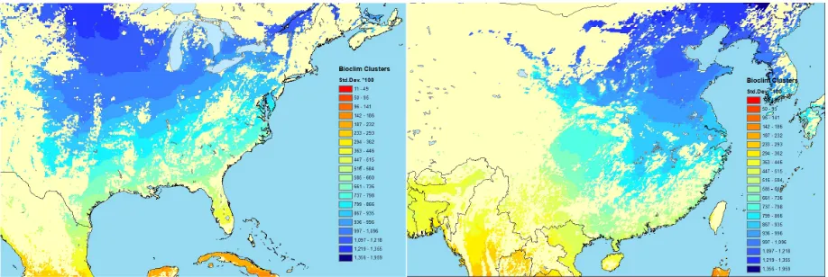
Figure 7. Classification of North America and East Asia cropland according to temperature seasonality variability (BIO4 variable from BIOCLIM).http://worldclim. org/bioclim
Testing effects of inclusion of geoclimactic features in predictive modelling of 529
phenotypic performance across geographies, bioclicmactic parameters from bioclim 530
have been used as features in machine learning algorithms across geographies (Martin 531
unpublished, Figure7). In anArabidopsis thalianacase study (Ersoz,2019) it was reported 532
that inclusion of the environmental features into a Random Forest prediction model 533
together with genetic features found no conclusive trends, since for some phenotypes 534
there was increase in prediction accuracy and at yet for others, a decrease was observed. 535
This was postulated to be due to the direction of the GxE parameters (un-adapted versus 536
well-adapted GxE combinations) that was not explicitly controlled in the model. More 537
work is needed to develop these models and evaluate their efficacy in crops. 538
Advancements in this exciting area requires not only private and public investments 539
organizations for public research and training. In recognition of this necessity, Syngenta 541
has been coordinating an annual crowd-sourcing analytics challange in partnership with 542
the Analytics Society of INFORMS since 2015. Examples of methods developed in these 543
contests, known as Syngenta-Informs Challanges are Marko et al. (2017) and Zhong
544
et al. (2018). More funding, public and private, and more data would enable future 545
innovations in this domain, as well as training of domain experts that can apply these 546
methods. 547
5. Machine Learning for Sustainable Agriculture
548
In addition to the geoclicmactic variables mentioned in the previous section (Figure 549
7), there are many other publicly available data resources that can be leveraged to 550
evaluate various characteristic of cropping systems versus geographies. 551
For example, USDA- Economic Research Service5compiles and distributes annual
552
data for land use and farm land utilization and management practices across the US 553
such as crop rotation and average reported yield per crop. USDA Pest Information 554
Platform for Extension and Education (PIPE)6collects and distributes pest and disease 555
data from across north america. National Centers of Environmental Information division 556
of National Oceanic and Atmospheric Administration (NOAA), collects and distributes 557
drought monitor and extreme climate event data7 and there are many others, that are 558
too numerous to cite here. We will refer to this collection of repositories and data as 559
biogeoclimactic datafor ease of reference. 560
Biogeoclimactic data can be compiled in such a way that each data layer, anchored to 561
geographic coordinates, may be treated as different layers of an image. Such restructuring 562
and compilation of this data would enable use of Convolutional Neural Networks 563
(CNNs), a tool designed for analysis of such layered data by developing ML models. 564
These models can then be leveraged not only to fine tune classification of adaptive 565
region definitions for existing varieties, but can also be leveraged to forecast suitability 566
of existing varieties based on changing bioclimactic conditions (e.g. What is the expected 567
performance for variety X in geography Y?, or what is the expected performance of 568
variety X with climactic parameter set Z?). These models can ultimately be used for 569
making management recommendations for optimizing on-farm management practices, 570
for increasing sustainability of agriculture and to improve margins for the growers. 571
Another potential approach to modelling biogeoclicmactic effects for crop 572
productivity is using the data without the discretization, on a continuous scale. 573
5 https://www.ers.usda.gov/data-products/data-visualizations/ 6 http://sbr.ipmpipe.org/cgi-bin/sbr/public.cgi
Continuous scale modelling would allow capturing influences of extreme-climate events, 574
i.e. droughts, floods, locust years, etc. without smoothing them over as regional averages 575
or discarding them as outliers. This can be achieved by Recurrent Neural Network 576
(RNN) Modelling, as these models seem to capture properties of such extreme weather 577
events (Saha and Mitra,2016). 578
6. Discussion
579
In this review, our objective was to present an overview of the current and potential 580
applications of predictive modelling with machine learning for its applications to 581
contemporary crop breeding and improvement. We started by emphasizing the fact that 582
crop improvement is inseparably tangled with geoclimactic adaptation, followed by a 583
discussion on available tools and strategies for predicting unobserved phenotypes under 584
various conditions to accelerate and inform variety development efforts. 585
We have also discussed leveraging bioclimactic classification methods and long term 586
geo-climactic data to inform variety development and placement as well as generating 587
forecasts for crop productivity under today’s rapidly changing environmental conditions. 588
We did not discuss genomics and biotechnology applications of ML & AI relevant 589
to breeding such as gene editing target identification, gene and allele discovery, or 590
leveraging crop-wild relatives for variety development. To do these topics justice, a 591
separate article would be warranted. 592
We also have not discussed the fine details of algorithmic and methodological 593
complexity of applications of machine learning approaches, since we are of the opinion 594
that such discussions would best be included in an actual investigation study rather then 595
a review ms. 596
Our intention was to keep this review focused on providing examples for how ML 597
and AI can help improve breeding logistics and operational challenges, thereby rate 598
of genetic gain in breeding programs for accelerated variety development. We have 599
also presented a case for leveraging this data and methods for enabling sustainable 600
agricultural practices by redefining and forecasting adaptive variety and management 601
recommendations for farmers. 602
We hope that the examples we provided here would serve and inspire the community 603
to develop and apply these novel models and methods in crop breeding in the near 604
future. 605
Funding: This research, and preparation of the manuscript was fully voluntary on the authors’ parts and no
606
external funding was received for NFM and ESE. This project was partially supported by National Research Initiative
607
Competitive Grant no. 2017-67013-26188 from the USDA National Institute of Food and Agriculture to AES.
608
Acknowledgments: We are grateful to Mark Cooper for asking us to contribute an ms to this special issue of Crop
609
Science, and providing recommendations as to its topic. The funders had no role in study design, data collection and
610
analysis,decision to publish, or preparation of the manuscript.
Conflicts of Interest: EE is the founder and Research Director for Umbrella Genetics, which is a for profit
612
organization that offers big data analytics services for agricultural product research and development. NFM was
613
the Chair of the Challenge Review Committee for Syngenta- Informs Challenge starting 2017 up to 2019. These
614
connections had no role in the collection, analyses, or interpretation of data presented here, other then as cited, or in
615
the writing of the manuscript, or in the decision to publish the ms.
616
References
617
Borlaug, N. Sixty-two years of fighting hunger: personal recollections. Euphytica 618
2007,157, 287 – 297. 619
Bullock, D. Crop rotation. Critical Reviews in Plant Sciences 1992, 11, 309–326, 620
[https://doi.org/10.1080/07352689209382349]. doi:10.1080/07352689209382349. 621
Kwon, S.; Torrie, J. Heritability of and Interrelationships Among Traits of Two 622
Soybean Populations 1. Crop science1964,4, 196–198. 623
Meredith, W.R.; Bridge, R. Breakup of Linkage Blocks in Cotton, Gossypium 624
hirsutum L. 1. Crop science1971,11, 695–698. 625
Kato, T.; Takeda, K. Associations among characters related to yield sink capacity in 626
space-planted rice. Crop science1996,36, 1135–1139. 627
Triboi, E.; Martre, P.; Girousse, C.; Ravel, C.; Triboi-Blondel, A.M. Unravelling 628
environmental and genetic relationships between grain yield and nitrogen 629
concentration for wheat. European Journal of Agronomy2006,25, 108–118. 630
Erskine, W.; Williams, P.C.; Nakkoul, H. Genetic and environmental variation in 631
the seed size, protein, yield, and cooking quality of lentils. Field Crops Research 632
1985,12, 153–161. doi:10.1016/0378-4290(85)90061-9. 633
Guanming, S.; Jean-paul, C.; Kyle, S. An Analysis of the Pricing of Traits in the U.S. 634
Corn Seed Market. American Journal of Agricultural Economics2010, p. 1324. 635
Reekie, E.; Bazzaz, F. Reproductive effort in plants. 2. Does carbon reflect the 636
allocation of other resources? The American Naturalist1987,129, 897–906. 637
Moose, S.P.; Dudley, J.W.; Rocheford, T.R. Maize selection passes the century 638
mark: a unique resource for 21st century genomics. Trends in Plant Science2004, 639
9, 358–364. doi:10.1016/j.tplants.2004.05.005. 640
Guo, Y.; Yang, X.; Chander, S.; Yan, J.; Zhang, J.; Song, T.; Li, J. Identification of 641
unconditional and conditional QTL for oil, protein and starch content in maize. 642
The Crop Journal2013,1, 34–42. doi:10.1016/j.cj.2013.07.010. 643
Li, Y.H.; Li, W.; Zhang, C.; Yang, L.; Chang, R.Z.; Gaut, B.S.; Qiu, L.J. Genetic 644
diversity in domesticated soybean (Glycine max) and its wild progenitor (Glycine 645
soja) for simple sequence repeat and single-nucleotide polymorphism loci. New 646
Phytologist2010,188, 242–253. doi:10.1111/j.1469-8137.2010.03344.x. 647
Reekie, E.; Bazzaz, F. Reproductive effort in plants. 1. Carbon allocation to 648
reproduction. The American Naturalist1987,129, 876–896. 649
Schoen, D.J.; Dubuc, M. The Evolution of Inflorescence Size and Number: A 650
Gamete-Packaging Strategy in Plants. The American Naturalist1990,135, 841–857. 651
Oury, F.X.; Godin, C. Yield and grain protein concentration in bread wheat: how to 653
use the negative relationship between the two characters to identify favourable 654
genotypes? Euphytica2007,157, 45–57. doi:10.1007/s10681-007-9395-5. 655
Rotundo, J.L.; Borrás, L.; Westgate, M.E.; Orf, J.H. Relationship between assimilate 656
supply per seed during seed filling and soybean seed composition. Field Crops 657
Research2009,112, 90–96. doi:10.1016/j.fcr.2009.02.004. 658
Piper, J.K.; Kulakow, P.A. Seed yield and biomass allocation in Sorghum bicolor 659
and F1 and backcross generations of S. bicolor×S. halepense hybrids. Canadian 660
Journal of Botany1994,72, 468–474. 661
Ledford, H. Fixing the tomato: CRISPR edits correct plant-breeding snafu. Nature 662
News2017,545, 394. doi:10.1038/nature.2017.22018. 663
Greene, S.L.; Khoury, C.K.; Williams, K.A., Wild plant genetic resources in North 664
America: an overview. InNorth American Crop Wild Relatives, Volume 1; Springer, 665
2018; p. 3–31. 666
von Wettberg, E.J.; Chang, P.L.; Ba¸sdemir, F.; Carrasquila-Garcia, N.; Korbu, L.B.; 667
Moenga, S.M.; Bedada, G.; Greenlon, A.; Moriuchi, K.S.; Singh, V.; others. Ecology 668
and genomics of an important crop wild relative as a prelude to agricultural 669
innovation. Nature communications2018,9, 649. 670
Van de Wouw, M.; Kik, C.; van Hintum, T.; van Treuren, R.; Visser, B. Genetic 671
erosion in crops: concept, research results and challenges. Plant Genetic Resources 672
2010,8, 1–15. 673
Li, L.; Zheng, W.; Zhu, Y.; Ye, H.; Tang, B.; Arendsee, Z.W.; Jones, D.; Li, R.; Ortiz, 674
D.; Zhao, X.; et al.. QQS orphan gene regulates carbon and nitrogen partitioning 675
across species via NF-YC interactions. Proceedings of the National Academy of 676
Sciences2015,112, 14734–14739. doi:10.1073/pnas.1514670112. 677
Soyk, S.; Lemmon, Z.H.; Oved, M.; Fisher, J.; Liberatore, K.L.; Park, S.J.; Goren, 678
A.; Jiang, K.; Ramos, A.; Knaap, E.v.d.; et al.. Bypassing Negative Epistasis on 679
Yield in Tomato Imposed by a Domestication Gene. Cell2017,169, 1142–1155.e12. 680
doi:10.1016/j.cell.2017.04.032. 681
Batista, L.; Gaynor, R.C.; Margarido, G.R.; Byrne, T.; Amer, P.; Gorjanc, G.; Hickey, 682
J.M. Plant breeders should be determining economic weights for a selection index 683
instead of using independent culling for choosing parents in breeding programs 684
with genomic selection. bioRxiv2018, p. 500652. 685
van Eeuwijk, F.A.; Bustos-Korts, D.V.; Malosetti, M. What Should Students in 686
Plant Breeding Know About the Statistical Aspects of Genotype Environment 687
Interactions? Crop Science2016,56, 2119–2140. doi:10.2135/cropsci2015.06.0375. 688
Doubler, T.W. The use of genetic information to predict the relative maturity of 689
soybeans. PhD thesis, IAState, Iowa State University Digital Repository, 2016. 690
Buckler, E.S.; Holland, J.B.; Bradbury, P.J.; Acharya, C.B.; Brown, P.J.; Browne, C.; 691
Ersoz, E.; Flint-Garcia, S.; Garcia, A.; Glaubitz, J.C.; et al.. The Genetic Architecture 692
of Maize Flowering Time. Science2009,325, 714–718. doi:10.1126/science.1174276. 693
Tenaillon, M.I.; Seddiki, K.; Mollion, M.; Guilloux, M.L.; Marchadier, E.; Ressayre, 694
in maize reveals convergence and key players of the underlying gene regulatory 696
network. bioarxiv. https://www.biorxiv.org/content/early/2018/11/23/461947,
697
2018. doi:10.1101/461947. 698
Ribaut, J.M.; Hoisington, D. Marker-assisted selection: new tools and strategies. 699
Trends in Plant Science1998,3, 236–239. doi:10.1016/S1360-1385(98)01240-0. 700
Gauffreteau, A. Using ideotypes to support selection and recommendation of 701
varieties. OCL2018,25, D602. doi:10.1051/ocl/2018042. 702
Tutino, C. Optimizing Breeding Process Builds Yield. Syngenta Thrive Magazine, 703
2016. 704
Lepore, J. What 2018 Looked Like Fifty Years Ago2018. 705
Meuwissen, T.H.E.; Hayes, B.J.; Goddard, M.E. Prediction of Total Genetic Value 706
Using Genome-Wide Dense Marker Maps. Genetics2001,157, 1819–1829.
707
Meuwissen, T.H.; Goddard, M.E. Prediction of identity by descent probabilities 708
from marker-haplotypes. Genetics, Selection, Evolution: GSE2001,33, 605–634. 709
doi:10.1186/1297-9686-33-6-605. 710
Peiffer, J.A.; Romay, M.C.; Gore, M.A.; Flint-Garcia, S.A.; Zhang, Z.; Millard, M.J.; 711
Gardner, C.A.; McMullen, M.D.; Holland, J.B.; Bradbury, P.J.; others. The genetic 712
architecture of maize height. Genetics2014,196, 1337–1356. 713
Ersoz ES, Myers C, K.D.e.a. Harnessing global genetic potential with CropOS. 714
F1000Research 2019, 8:202 (poster) https://doi.org/10.7490/f1000research.
715
1116445.1, 2017. 716
Moser, G.; Lee, S.H.; Hayes, B.J.; Goddard, M.E.; Wray, N.R.; Visscher, P.M. 717
Simultaneous Discovery, Estimation and Prediction Analysis of Complex 718
Traits Using a Bayesian Mixture Model. PLOS Genetics 2015, 11, e1004969.
719
doi:10.1371/journal.pgen.1004969. 720
Voss-Fels, K.P.; Cooper, M.; Hayes, B.J. Accelerating crop genetic gains with genomic 721
selection. Theoretical and Applied Genetics2018. doi:10.1007/s00122-018-3270-8. 722
Gorjanc, G.; Gaynor, R.C.; Hickey, J.M. Optimal cross selection for long-term genetic 723
gain in two-part programs with rapid recurrent genomic selection. Theoretical and 724
Applied Genetics2018,131, 1953–1966. 725
Dimitrijevic, A.; Horn, R. Sunflower hybrid breeding: from markers to genomic 726
selection. Frontiers in plant science2018,8, 2238. 727
Ozimati, A.; Kawuki, R.; Esuma, W.; Kayondo, S.I.; Pariyo, A.; Wolfe, M.; Jannink, 728
J.L. Genetic Variation and Trait Correlations in an East African Cassava Breeding 729
Population for Genomic Selection. Crop Science2019. 730
Rio, S.; Mary-Huard, T.; Moreau, L.; Charcosset, A. Genomic selection efficiency 731
and a priori estimation of accuracy in a structured dent maize panel. Theoretical 732
and Applied Genetics2019,132, 81–96. 733
Sweeney, D.W.; Sun, J.; Taagen, E.; Sorrells, M.E. Genomic Selection in Wheat. In 734
Heslot, N.; Yang, H.P.; Sorrells, M.E.; Jannink, J.L. Genomic Selection in 736
Plant Breeding: A Comparison of Models. Crop Science 2012, 52, 146.
737
doi:10.2135/cropsci2011.06.0297. 738
Kemper, K.E.; Bowman, P.J.; Hayes, B.J.; Visscher, P.M.; Goddard, M.E. A multi-trait 739
Bayesian method for mapping QTL and genomic prediction. Genetics Selection
740
Evolution2018,50, 10. doi:10.1186/s12711-018-0377-y. 741
Moore, J.H.; Olson, R.S.; Schmitt, P.; Chen, Y.; Manduchi, E. How computational 742
thought experiments can improve our understanding of the genetic architecture 743
of common human diseases. The 2018 Conference on Artificial Life: A Hybrid of 744
the European Conference on Artificial Life (ECAL) and the International Conference 745
on the Synthesis and Simulation of Living Systems (ALIFE) 2018, p. 23–30. 746
doi:10.1162/isal_a_00012. 747
Harper, W.R.; Harris, D.H. The Application of Link Analysis to Police Intelligence. 748
Human Factors1975,17, 157–164,[https://doi.org/10.1177/001872087501700206]. 749
doi:10.1177/001872087501700206. 750
Page, L.; Brin, S.; Motwani, R.; Winograd, T. The PageRank Citation Ranking: 751
Bringing Order to the Web. Technical Report 1999-66, Stanford InfoLab, 1999. 752
Previous number = SIDL-WP-1999-0120. 753
Park, J.; Yook, S.H. Bayesian Inference of Natural Rankings in Incomplete
754
Competition Networks. Scientific Reports2014,4, 6212. doi:10.1038/srep06212. 755
Simko, I.; Pechenick, D.A. Combining partially ranked data in plant breeding and 756
biology: I. Rank aggregating methods. Communications in Biometry Crop Science 757
2010,5, 41 – 55. 758
Lande, R.; Thompson, R. Efficiency of marker-assisted selection in the improvement 759
of quantitative traits. Genetics1990,124, 743–756. 760
Haley, C.S.; Visscher, P.M. Strategies to Utilize Marker-Quantitative
761
Trait Loci Associations. Journal of Dairy Science 1998, 81, 85–97.
762
doi:10.3168/jds.S0022-0302(98)70157-2. 763
Ribaut, J.M.; Ragot, M. Marker-assisted selection to improve drought adaptation in 764
maize: the backcross approach, perspectives, limitations, and alternatives. Journal 765
of Experimental Botany2006,58, 351–360. doi:10.1093/jxb/erl214. 766
Togashi, K.; Lin, C.Y. Theoretical efficiency of multiple-trait quantitative trait 767
loci-assisted selection. Journal of Animal Breeding and Genetics2010,127, 53–63. 768
doi:10.1111/j.1439-0388.2009.00817.x. 769
Hospital, F. Selection in backcross programmes. Philosophical Transactions of the 770
Royal Society B: Biological Sciences2005,360, 1503–1511. doi:10.1098/rstb.2005.1670. 771
Ragot, M.; Biasiolli, M.; Delbut, M.; Dell’Orco, A.; Malgarini, L.; Thevenin, P.; 772
Vernoy, J.; Vivant, J.; Zimmermann, R.; Gay, G. Marker-assisted backcrossing: a 773
practical example. COLLOQUES-INRA1995, pp. 45–45.
774
Collard, B.C.; Mackill, D.J. Marker-assisted selection: an approach for precision 775
plant breeding in the twenty-first century. Philosophical Transactions of the Royal 776
Wallace, J.G.; Rodgers-Melnick, E.; Buckler, E.S. On the Road to Breeding 4.0: 778
Unraveling the Good, the Bad, and the Boring of Crop Quantitative Genomics. 779
Annual review of genetics2018,52, 421–444. 780
Evans, J. Optimization algorithms for networks and graphs; Routledge, 2017. 781
Festa, P. The shortest path tour problem: problem denition, modeling, and 782
optimization. e-book semanticscholar.org https://pdfs.semanticscholar.org/
783
d2f6/39c285fe6f1f549b403aa52f9c22ecc5e37e.pdf, 2019. 784
Ritchie, S.W.; Chintamanani, S.P.; Dunn, M.; Ersöz, E.S.; Foster, D.J.; Martin, N.F.; 785
Skibbe, D.S.; Tucker, D.M. Genetic Markers Associated with Increased Fertility in 786
Maize, 2017. US Patent App. 15/117,491. 787
Fedoryuk, M. Asymptotic methods in analysis. InAnalysis I; Springer, 1989; pp. 788
83–191. 789
Smirnov, V. On the estimation of a path integral by means of the saddle point 790
method. Journal of Physics A: Mathematical and Theoretical2010,43, 465303. 791
Ruder, S. An overview of gradient descent optimization algorithms. arXiv preprint 792
arXiv:1609.047472016. 793
Sebastiani, F. Machine learning in automated text categorization. ACM computing 794
surveys (CSUR)2002,34, 1–47. 795
Ortiz, R.; Crossa, J.; Franco, J.; Sevilla, R.; Burgueño, J. Classification of Peruvian 796
highland maize races using plant traits. Genetic Resources and Crop Evolution2008, 797
55, 151–162. 798
Grobman, A. Races of maize in Peru: their origins, evolution and classification; Vol. 915, 799
National Academies, 1961. 800
Wright, K.R.; Wright, R.M.; Valencia, Z.; McEwan, G.F.; others. Moray: Inca
801
engineering mystery.; American Society of Civil Engineers (ASCE), 2010. 802
Cooper, M.; Messina, C.D.; Podlich, D.; Totir, L.R.; Baumgarten, A.; Hausmann, N.J.; 803
Wright, D.; Graham, G. Predicting the future of plant breeding: complementing 804
empirical evaluation with genetic prediction. Crop and Pasture Science 2014, 805
65, 311–336. 806
Byrum, J.; Davis, C.; Doonan, G.; Doubler, T.; Foster, D.; Luzzi, B.; Mowers, 807
R.; Zinselmeier, C.; Kloeber, J.; Culhane, D.; others. Advanced analytics for 808
agricultural product development. Interfaces2016,46, 5–17. 809
Kang, M.S. Using genotype-by-environment interaction for crop cultivar
810
development. InAdvances in agronomy; Elsevier, 1997; Vol. 62, pp. 199–252. 811
Löffler, C.M.; Wei, J.; Fast, T.; Gogerty, J.; Langton, S.; Bergman, M.; Merrill, B.; 812
Cooper, M. Classification of maize environments using crop simulation and 813
geographic information systems. Crop Science2005,45, 1708–1716. 814
Crossa, J.; Fox, P.; Pfeiffer, W.; Rajaram, S.; Gauch, H. AMMI adjustment for 815
statistical analysis of an international wheat yield trial. Theoretical and Applied 816
Genetics1991,81, 27–37. 817
Messina, C.D.; Podlich, D.; Dong, Z.; Samples, M.; Cooper, M. Yield–trait
818
performance landscapes: from theory to application in breeding maize for drought 819