Millimetric Diagnosis: Machine Learning Based Network Analysis for mm-Wave Communication

Millimetric Diagnosis: Machine Learning Based

Network Analysis for mm-Wave Communication

Maria Scalabrin and Michele Rossi

Guillermo Bielsa, Adrian Loch, and Joerg Widmer

Avda. del Mar Mediterraneo 22, 28918 Leganes, Madrid, Spain email: {guillermo.bielsa, adrian.loch, joerg.widmer}@imdea.org

Abstract—Troubleshooting millimeter-wave (mm-wave) wire-less networks is complex due to the directionality of the communi-cation. Issues such as deafness, misaligned antennas, or blockage may severely impact network performance, and identifying them is crucial to improve network deployments. To this end, access to lower-layer information is important. However, commercial off-the-shelf mm-wave wireless devices typically do not provide such information. Even if they would, detecting effects such as deafness based on information of a single node that forms part of the network is typically hard. In this paper, we present the design and evaluation of an external sniffing device that can infer the aforementioned performance issues only using narrowband physical layer energy traces. Our sniffer does not need to decode any data, resulting in a simple but effective approach which also preserves privacy and works on encrypted networks. Our key contribution is a machine learning framework which enables automated energy trace analysis while coping with the non-stationarity of the traces. We evaluate its performance in practice using off-the-shelf wireless devices operating in the 60 GHz band. Our results show that the above framework correctly infers physical layer events in virtually all cases, thus providing valuable information to troubleshoot issues in mm-wave networks.

I. INTRODUCTION

The directional nature of millimeter-wave (mm-wave) com-munications results in issues that strongly impact higher layers but which are hard to identify without detailed information of the underlying physical layer effects. This includes, for instance, deafness [1], misaligned antennas, and link blockage. Unfortunately, Commercial Off-The-Shelf (COTS) devices are typically a black box regarding such physical layer infor-mation. As a result, troubleshooting COTS-based, real-world mm-wave network deployments often translates into time-consuming “trial-and-error” analysis. While understanding performance issues in such deployments is challenging [2]– [4], the resulting knowledge is extremely valuable. It provides useful insights for network planners and administrators, such as giving advice on whether an Access Point (AP) should be relocated to prevent harmful reflections. Moreover, this knowl-edge helps researchers to understand and improve protocol de-sign, analyze performance of new mechanisms, and investigate standard compliance of mm-wave devices. However, gaining such insights from a COTS node that forms part of the network is virtually impossible. On top of the aforementioned lack of lower-layer access, a single node would be restricted to its

250 500 750 1000 1250 1500

Sample number

0 0.1 0.2 0.3

Amplitud

e [V]

Control Packets

(Beacon Pair) Data Packet and Acknowledgment Exchanges

Fig. 1. Energy trace example of a data burst starting with a pair of beacons.

particular point of view—the directivity of the communication limits the insights that we could gain. To prevent this, we need to capture and compare the behavior of the network from multiple points of view. Given the extreme bandwidth available in mm-wave communications (e.g., 2 GHz per channel in the 60 GHz band), this requires an inordinate amount of data processing, and thus would be highly challenging.

In this paper, we design and evaluate an automated mm-wave network diagnosis tool based on COTS hardware that overcomes the above limitations. Specifically, the tool uses machine learning techniques to infer performance bottlenecks in 60 GHz networks using narrowband physical layer en-ergy traces from one or more sniffers. That is, we do not record and decode the full communication but only require the energy level that the sniffers receive. While sniffers are directional, by combining the traces of multiple sniffers we can obtain the full picture of network activity. The result is an energy trace as shown in Fig. 1. This trace depicts the start of a typical data burst in IEEE 802.11ad. The data burst starts with a pair of beacons which contain control information. The pair of beacons is followed by a sequence of data packets and acknowledgments. While not shown in Fig. 1, occasional Beam Refinement (BR) sequences retrain the antenna beams in case of, for instance, node movement, to ensure that both nodes remain in the boresight of each other. By means of simple visual inspection, it is easy to identify the individual frame types in the trace. This enables us to infer the dynamics of the communication. For instance, a missing acknowledgment after a data packet hints at a deafness issue, overlapping packet frames suggest a collision, and so on. While this is visually evident, manually inspecting the energy traces is clearly infeasible given the number of packets when

communicating at multi-gigabit-per-second rates. At the same time, finding such events in an automated manner is hard. Our key contribution is developing a machine learning framework that is able to correctly classify the above frame types and infer network issues. This is far from trivial due to (a) the non-stationarity of the traces and (b) the complexity of the IEEE 802.11ad protocol [5]. To address (a), we dynamically update the parameters of the underlying machine learning model such that it adjusts to variations in the received energy level due to, e.g., node movement. Regarding (b), we use a combination of template matching and an Explicit Duration Hidden Markov Model (EDHMM) to correctly classify frames.

The core idea of our approach is also applicable to networks operating at lower frequencies such as IEEE 802.11ac. Still, in this paper we focus on the mm-wave case, which is more challenging due to the use of directional antennas and the large bandwidth. Since we do not need to decode any of the data, our approach preserves privacy, works regardless of whether the network uses encryption, and does not require accurate time/frequency synchronization. As a result, our technique is simple yet highly effective. Our contributions are as follows:

• We design a machine learning framework based on tem-plate matching and an EDHMM to diagnose physical layer issues in 60 GHz networks. The main challenge lies in the variability of the traces and the complexity of identifying the structural elements in the traces given their noisiness, aperiodicity, and unpredictable behavior. Standard machine learning approaches fail in such a scenario. The key to solve this issue is the aforementioned complex combination of machine learning techniques. • We introduce a time-adaptive learning mechanism to cope

with the non-stationarity of energy traces due to gain control adjustments and node movement. This run-time adaptation is barely explored in specialized work in the field of statistics but is critical for the success of our approach. It sets our work apart from existing work based on simple clustering or thresholding which is highly sensitive to non-stationary behavior and thus often fails. • We evaluate our approach in an extensive measurement campaign using COTS 60 GHz hardware to analyze its performance in a range of practical scenarios.

The remainder of this paper is structured as follows. In Section II we survey related work, and in Section III we provide some preliminaries of our EDHMM. We then give an overview of our machine learning framework in Section IV, and delve into its details in Sections V and VI. In Section VII we introduce the aforementioned time-adaptive learning mech-anism. After that, we present and discuss our evaluation results in Section VIII, and conclude the paper in Section IX.

II. RELATEDWORK

In the following, we give an overview of performance analy-sis and troubleshooting in mm-wave networking. As sketched in Section I, mm-wave networks suffer from high path-loss and high absorption. To overcome this, nodes typically use directional antennas and Line-Of-Sight (LOS) paths. However,

this makes links very susceptible to blockage. State-of-the-art work in this field [6]–[8] focuses on correctly identifying such blockage at the nodes involved in the communication, and reacting in a timely manner. For instance, BeamSpy [7] measures the set of available paths between a transmitter and a receiver. This “path skeleton” serves as a reference whenever blockage occurs—the nodes compute which of the paths in the skeleton is most likely to be unaffected by the blockage and steer their antennas accordingly. As a result, BeamSpy can avoid costly beam steering overhead. Further, earlier work by the same authors [8] looks into differentiating device move-ment from blockage based on Received Signal Strength (RSS) measurements. This is key to ensure that nodes react correctly when links degrade. Similarly, MOCA [6] transmits a very short control message to assess the link state. If the transmitter does not obtain a reply, it assumes that the antennas are misaligned. Otherwise, it adapts the Modulation and Coding Scheme (MCS) according to the current channel state. All of the above approaches aim at improving the performance of mm-wave networks. In contrast, our work troubleshoots the operation of such approaches and is thus orthogonal to them. While BeamSpy and MOCA also try to identify specific issues in the communication, they are constrained to the specific “viewpoint” of a certain node. Our framework runs on one or more external sniffers which we can place at multiple locations, thus providing much richer insights. Moreover, the sniffers are only needed while troubleshooting the network but not during regular operation.

Earlier work proposes an equivalent concept based on external sniffers. However, such approaches typically consider lower frequency bands, and focus on security issues [9], [10] such as realizing an Intrusion Detection System (IDS). The key difference to our approach is that such security sniffers are designed to continuously operate along with the network, thus increasing the complexity of the deployment. In contrast, our tool does not need to be part of the network, and can be used on-demand only. Hence, we do not add complexity to the network. Moreover, we focus on performance issues in directional wireless networks while the above work deals with security in the omni-directional case. However, [10] and references therein also deal with raw physical layer data, similarly to our case. Specifically, they suggest overhearing the communication and jamming unwanted packets based on, for instance, header information. Our tool also overhears the communication but does not need to decode any preambles and headers to identify the start and source of the packets, respectively. Instead, we use machine learning on the timing of frames to obtain the information required for network analysis. Our tool is the first automatic classifier of IEEE 802.11ad energy traces for network diagnosis. The uniqueness of our approach prevents direct comparison with earlier work.

which are particularly complex and resource intensive in mm-wave networks. However, this poses additional challenges such as identifying frames and discerning which node transmits which frame. In this paper, we provide solutions to these challenges. This contribution sets us apart from existing work.

III. EDHMM PRELIMINARIES

We use uppercase and calligraphic fonts for sets, except for N(X;µ, σ2_{), which refers to a Gaussian random variableX}

with meanµand varianceσ2_{. We denote a random sequence of}

lengthT byX1:T = (X1, . . . , XT), where the random variable Xtat time indext∈ {1, . . . , T}takes values in the setX, with cardinality|X |. Realizations are indicated by lowercase letters, i.e.,xtis the realization ofXt, and withx1:T = (x1, . . . , xT)

we denote a sequence of realizations. Vectors are indicated by bold letters, e.g., bbb, and we refer to their elements asbbb= [b1, . . . , bK], with |bbb| = K. For matrices we use uppercase

bold letters, e.g.,AAA={aij} is a matrix with elementsaij.

Markov models, whose states correspond to observable events, are inadequate to solve our mm-wave channel estima-tion problem. The reason is that we measure a noisy version of the real state (i.e., the current energy level), as the transmitted energy levels are corrupted by random channel fluctuations. Instead, HMMs [13] are a more appropriate tool, as their observations are probabilistic functions of the (hidden) state. Specifically, a HMM is composed of embedded stochastic processes, where an unobservable hidden random process is revealed to the observer through another set of random processes that produce the sequence of observations. We now consider a data burst and aim to solve the following estimation problem. The observed channel samples in the data burst,

O1:T = (O1, . . . , OT), are modeled as a sequence of

real-valued random variables corresponding to one of the following basic elements: “1” inter-frame space (IFS), “2” data packet (DATA) and “3” acknowledgement (ACK). Accordingly, the hidden state St at time t is a discrete random variable that can take values in the set S = {1,2,3}. We define S1:T = (S1, . . . , ST)as the sequence of random variables describing

the hidden states in the data burst, i.e.,t∈ {1, . . . , T}. Our ob-jective is then to reliably estimate the sequence of hidden states

s1:T = (s1, . . . , sT) from observations o1:T = (o1, . . . , oT).

The standard HMM makes two basic assumptions regarding the embedded stochastic processes:

A1) The first assumption is thatS1:T is a first-order Markov

chain, i.e., P(St+1|S1, . . . , St) = P(St+1|St). In

par-ticular, we have P(St+1 = j|St = i) = aij, where A

A

A = {aij}, i, j ∈ S, is the single-step transition probability matrix of the HMM.

A2) The second assumption is that the random variableOtis

statistically independent of (O1, . . . , Ot−1).

Moreover, Ot is a probabilistic function of the hidden state

St, i.e., it obeys a suitable conditional probability P(Ot|St)

and each random variable Ot can use a private distribution P(Ot|St)over the hidden state. We use a Gaussian observation

model with P(Ot|St=i) =N(Ot;µi, σi2), whereµi andσ2i

specify the mean and the variance of the random variable Ot,

given that the hidden state is i ∈ S. This is known to well approximate the noise distribution for mm-wave channels [14]. For all hidden states i ∈ S, we collect the parameter pairs

bi = (µi, σ2_i) through vector bbb = [b1, . . . , b|S|]. We define πππ= [π1, . . . , π|S|], where πi is the probability that the HMM is in state i∈ S in the first time slot of the burst.

The HMM model is described through a further parameter vectorΘ= [πππ, AAA, bbb]. Its maximum likelihood estimate given a sequence of observations is obtained through the Expectation-Maximization (EM) algorithm [15], which entails two-step iterations. First, initial values for Θ are chosen, and using assumptions A1 and A2 the posterior distribution for the whole sequenceP(S1:T|O1:T,Θ)is computed. Hence, this posterior

is used to compute the expected log-likelihood (which is also known as the Baum’s auxiliary function) as

Q(Θnew,Θ) =X

S1:T∈ST

P(S1:T|O1:T,Θ) logP(S1:T, O1:T|Θnew).

(1)

Q(Θnew,Θ) is finally maximized with respect to Θnew, obtaining a new estimate for the HMM model. This pro-cess is repeated until convergence to a critical point. A proper initialization of Θ (with particular regard for bbb) is crucial for a proper convergence of the EM algorithm. For a Gaussian-observation model, applying the two-step itera-tions of the EM algorithm is equivalent to using the fol-lowing Baum’s reestimation approach [16]. Consider two new variables ξt(i, j) and γt(i), with i, j ∈ S, that are defined as ξt(i, j) =P(St=i, St+1=j|O1:T,Θ) and γt(i) =P|S|

j=1ξt(i, j). We have: π_inew = γ1(i)

anew_ij =

PT−1

t=1 ξt(i, j)

PT−1

t=1 γt(i)

µnew_i =

PT

t=1γt(i)ot

PT

t=1γt(i)

σ2 new_i =

PT

t=1γt(i)(ot−µi) 2

PT

t=1γt(i)

(2)

where ξt(i, j) and γt(i) are computed using the Forward-Backward algorithm, see [17], [18].

However, standard HMMs are insufficient for our pur-pose. In fact, the duration distribution for any hidden state

St=i∈ Swith self transition probabilityaiiis the geometric Probability Mass Function (PMF) g(d) = (aii)d−1_(1−aii),

and we found it to be unsuitable to model the duration of the states IFS, DATA and ACK. To address this, we consider the EDHMM, where for each hidden state i ∈ S we have

aii = 0 and a state-specific distribution pi(d) is specified over the discrete set Di = {dmini , . . . , d

max

i }, where d min i

and dmax_i are the minimum and maximum durations for the protocol element transmitted when in state i. Hence, upon entering state i ∈ S, the sequence of observations in that state is i.i.d., of length d ∈ Di (sampled from pi(d)), and

is emitted from P(Ot|St=i) =N(Ot;µi, σi2). The duration

Filtering & Downsampling

Template Matching

Pre-processing Data Bursts

Raw Channel Trace

Beacon Seqs y

y

y y˜yy _o(n)

1:Tn

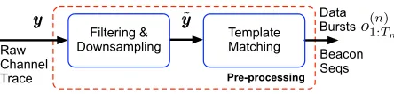
Fig. 2. Flow diagram of the mm-wave channel pre-processing phase.

p p

p = [p1(·), . . . , p|S|(·)]. The EDHMM model is described through the new parameter vector ΘEDHMM= [πππ, AAA, bbb, ppp].

IV. HIGHLEVELDESCRIPTION OF THE MM-WAVE

CHANNELESTIMATIONFRAMEWORK

The aim of the mm-wave channel analyzer that we present in this paper is twofold. First, we want to track when data bursts are transmitted and, for each, detect which packets are exchanged, their duration, and average energy. This allows obtaining statistics on their number, duration, whether there are channel problems (which may be detected from missing ACKs) and also allows tracking the channel quality (from variations in the energy levels). As a second objective, we track the transmission of control packets, which are sent for link management purposes. These control packets appear in two flavors as follows:

C1) The beacon pairs mark the beginning of a data burst. C2) The BR sequences are utilized to manage the radio link. Our approach consists of three steps.

Step 1 – Pre-processing (Fig. 2): beacon detection and data burst extraction are implemented through the pre-processing chain of Fig. 2, which operates on the raw channel trace, through filtering, downsampling and template matching, see Section V. We design the pre-processing chain for the case of 802.11ad but we can easily adapt it to suit other protocols. This pre-processing phase identifies all the beacons, classifies their occurrences into C1 and C2 and outputs a collection of

N data bursts of the form {o(_1:n_T)

n|n = 1, . . . , N}, which are

disjoint and contiguous channel subsequences.1

After Step 1, we delve into the semantic decoding of the protocol elements that are transmitted within each data burst, i.e., the elements in the above defined set S. To assess which elements are transmitted, along with their average energy and timing, we utilize an EDHMM model, which is first trained (Fig. 3), and then used at runtime (Fig. 4) with non-stationary traces. Let yyy = (y1, y2, . . .) be a sequence of channel

samples. In general, yyy can be written as yyy =xxx+www, where

x x

x= (x1, x2, . . .)is the signal of interestat the receiver, that

is, after transmission, andwww= (w1, w2, . . .)is the background

noise. From our experimental measurements, we know that

y y

y is highly non-stationary across data bursts, i.e., there are substantial variations in the energy associated with the signal

x x

x and the noisewww, which entail changes in µi and σ2 i, for i ∈ S. Moreover, they can also be caused by power control

1_{A contiguous subsequence is made up of consecutive channel samples.}

adjustments to compensate for channel attenuation and device mobility. Nevertheless, the transmission time of the elements in setS are channel and protocol-specific, as the transmission time of data frames may be adapted by the protocol according to the channel state. We proceed through the following steps.

Step 2 – EDHMM training (Fig. 3): we use stationary

channel traces for a preliminary and robust training of the EDHMM parameters. Channel traces were picked so as to encompass a wide range of data rates and MCSs, which de-termine the different lengths of the physical layer data frames. The distance between transmitter and receiver is kept fixed and the surrounding environment (indoor for our experiments) is kept as stable as possible (i.e., no user mobility, etc.). From these stationary channels, the state-specific distributions

pi(d) for i ∈ S do not undergo major changes during each trace and this allows their accurate estimation. Then, all the trace-specific distributions are combined into an “average” distribution considering a wide range of protocol settings, see Section VI. Note that training is needed only once for a given technology (e.g., 802.11ad).

Step 3 – Runtime trace analysis (Fig. 4): the EDHMM

parameters µi and σ_i2, for i ∈ S do depend on channel attenuation and noise. Thus, these parameters are estimated at runtime for each data burst using a clustering algorithm, whereas the pi(d) are known from Step 2. The so obtained

EDHMM model is used to estimate the most likely sequence inS (called the Viterbi path) from the samples in the current data burst. This step is explained in Section VII.

Steps 2 and 3 rely on the further assumption that:

A3) Channel attenuation and noise are stationary within bursts.

V. PRE-PROCESSING

HMM training Raw Channel

Trace

EDHMM initialization

Pre-processing State duration

estimates

EDHMM model refinement

EDHMM training y

yy o(_1:n_T)

n Θ

?

HMM ppp Θ

? EDHMM

Fig. 3. EDHMM training procedure: initial state duration estimates are obtained through HMM training and are refined using EDHMM learning tools.

Gaussian Observation Model Update Raw Channel

Trace

Runtime trace analysis Pre-processing

Online Estimation via Time-Adaptive

EDHMM

Performance Analysis y

yy o(_1:n_T)

n Θ

(n) EDHMM

Fig. 4. EDHMM runtime mm-wave channel analysis.

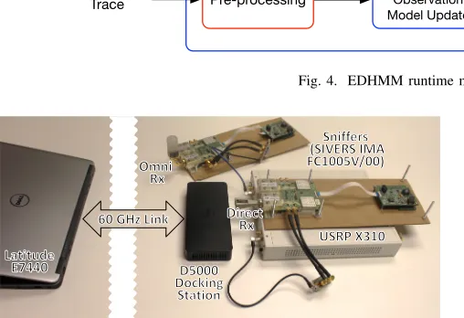
Fig. 5. Practical sniffer setup for trace capture. The antennas at the sniffers can be both directional or omni-directional, and sniffer location can be varied.

raw traceyyy is first filtered and then downsampled to a lower rate for scaling purposes, so that each sample of the new trace is computed as the mean of three subsequent samples in the original raw trace. This new trace is then smoothed using a fast and robust discretized spline filtering algorithm for data of high dimension [19] [20], thus obtaining the traceyyy˜.

Template Matching Algorithm: after the data acquisition, filtering, and downsampling, a collection of N data bursts of the form{o(_1:n_T)

n|n= 1, . . . , N}is extracted from the mm-wave

traceyy˜y. This requires a reliable identification technique for the data bursts and, recalling that each data burst is preceded by a pair of beacons, this corresponds to reliably detecting beacon pairs. What we observe from the collected channel traces is that the beacon duration and the inter-frame spacing between them are almost constant within and across experiments. Moreover, we note that the beacon shape is quite particular, showing different energy levels at the beginning and at the end. These characteristics make it possible to exploit a template matching technique for the beacon detection. Here, we are interested in finding C1) beacon pairs, and C2) BR sequences, as these are key to understand the protocol behavior.

At the core of our template matching approach, we use the Pearson’s correlation coefficient r ∈ [−1,1] [21], which is a statistical measure of the strength of a linear relationship between two vectorsuuu= [u1, . . . , uK] andvvv = [v1, . . . , vK]

(with meanµu andµv, respectively). It is defined as the ratio

of their covariance Cuv and the square root of the product of

their variancesσ2

u andσv2, i.e.,r=Cuv/(σuσv)is the sample

covariance given by:

Cuv= 1

K−1

K

X

k=1

(uk−µu)(vk−µv). (3)

The Pearson’s correlation coefficient is suitable to deal with the non-stationarity of the traces, since it just evaluates some internal relationship between the provided vectors. Moreover, template matching is known to be the optimal detection technique in the presence of white Gaussian noise [22], which we found to be a good assumption for our mm-wave channel traces [14]. Henceforth, for our template matching technique,

uuu corresponds to the average shape of a beacon frame (i.e., the template with a length of K samples), which the system can easily obtain from channel idle times. During those idle times, nodes only transmit periodic beacons which can be clearly identified and used as a template. Vector vvv contains the channel samples from the current K-dimensional sliding window, which moves over the signal traceyy˜y, obtained after the acquisition, filtering and downsampling ofyyy. We adopted the fast template matching scheme of [23] [24], which exploits the Fast Fourier Transform (FFT), thus obtaining dot products in the frequency domain. For a generic channel sequenceyy˜yof

L > Ksamples, this allows the computation of the covariance in O(LlogL) time. Hence, the template matching operates on y˜yy= (˜y1, . . . ,y˜L), outputting a sequence of correlation

estimates (r1, . . . , rL−K+1). We detect a possible beacon at

sample ` if r` is greater than a threshold rth. Then, since

multiple trivial matches (i.e., r` > rth) are likely to occur

across all our experiments settingrth= 0.75. Note thatrth is

independent of the trace amplitude. Thus, we do not need to readjust it for each scenario and/or trace.

The identification of pairs of beacons (C1) allows extracting the data bursts{o(_1:n_Tn) |n= 1, . . . , N}fromyy˜y, which are fed as input to the following EDHMM training phase. Longer beacon sequences (C2) are likewise detected by looking at the number of energy levels of the beacons therein and at their inter-frame spacing, as dictated by the standard [25]. These events are semantically decoded as described below.

VI. EDHMM TRAINING

For the EDHMM training we refer to Fig. 3. We recall that the objective of this training phase is to reliably estimate the distribution vector ppp, modeling the duration of inter-frame spaces, packets and acknowledgements. This phase is executed once offline and is not scenario dependent. Essentially, it is a calibration step for the specific mm-wave technology used in the network, which in our case is IEEE 802.11ad. The traces used in this step should be as much as possible stationary. This means that µi and σi2 do not significantly

vary across data bursts. As a first processing stage, we use the pre-processing procedure of Section V, which returns the data burst set{o(_1:n_Tn) |n= 1, . . . , N}. Next, for illustration purposes

we refer to the n-th data burst o(_1:n_T)

n = (o1, . . . , oTn), but

in our implementation the HMM parameters are estimated using the entire burst set (i.e., the N bursts in the mm-wave trace). For burst n, each of the samples ot, t = 0, . . . , Tn,

maps to an element st∈ S, where state “1” means IFS, “2”

DATA and “3” ACK. Our goal is to accurately associate each

ot in the data burst with the actual protocol element i ∈ S

and, most importantly, to reliably estimate its duration PMF

pi(·). This estimation is performed having access to the noisy observations (o1, . . . , oTn)of the actual protocol elements.

EDHMM initialization: we consider o(_1:n_Tn) as training data and our aim is to get accurate state duration estimates for the EDHMM. This is achieved by deriving initial estimates forppp

through a simpler HMM model. Once this vector is found, it is refined using EDHMM training tools. The HMM parameter vector is ΘHMM and the three fundamental steps involved in

the HMM model estimation are:

E1) The forward-backward algorithm is used to compute metricsγt(i)andξt(i, j)witht= 1, . . . , Tn,i, j∈ S(see

Eq. (2)) for a given HMM transition structure and a list of observations. These weigh the probability of getting the observed sequence from the current model.

E2) The model parameter vector ΘHMM is adjusted through

the EM algorithm.

E3) The Viterbi algorithm [26] is used to compute the most probable path via a Maximum Likelihood (ML) approach. Step E2 returns the optimal parameter vectorΘ?_HMM, whereas E3 outputs the sequence of hidden states (s1, . . . , sTn) that

most likely generated the observed samples (o1, . . . , oTn).

Specifically, we assume π1= 1 as all the data bursts start

with a silence, right after the beacon pair. Moreover, the HMM

transition matrixAAAis constrained in the sense that the hidden state sequence evolves according to structured trajectories [27]. In particular, we havea23=a32= 0, as there must be some

minimum inter-frame spacing between subsequent messages. Also, we setaii= 1−1/Tsfori∈ S, whereTs= 0.1µs is the channel sampling period after the downsampling of Section V. This implies a geometrically distributed dwell time in each state. Still, it serves as a sufficiently good initialization of the transition matrix and increases the HMM models robustness against random fluctuations in the channel dynamics.

The final parameter estimates Θ?_HMM strongly depend on the initial vectorΘ0_HMM for the EM evaluation (step E2). To obtain good initial parameter estimates, we use the K-means clustering algorithm, see [28], [29], which classifies the chan-nel samples in the data bursts around |S| centers. The |S| initial values of the centers can be randomly picked or taken as the locations of the peaks in the empirical distribution of the observed samples. The latter approach was implemented and found to perform satisfactorily across all datasets. Upon completion, theK-means algorithm returns|S|values for the cluster centers, which are used as initial values for µi for

i∈ S. The|S| variancesσ2_i are derived from the distribution of the samples clustered around the centersµi so obtained.

At this point, we use the Viterbi algorithm output (step E3) to fit |S| two-parameter inverse Gaussian distributions [30] [31] for vectorppp, where the rangeDi={dmini , . . . , dmaxi }

for state i ∈ S is such that dmin

1 = · · · = dmin|S| = 1 and dmax

1 =· · ·=dmax|S| =D. In particular, we setD according to the timing parameters of the IEEE 802.11ad communication standard [25] and filter out all the state durations that are outside these boundaries.

EDHMM model refinement: the initial estimate ppp that we have found with the above HMM model is subsequently refined through EDHMM training tools. Here, we opted for the forward-backward algorithm proposed by Yu and Kobayashi in [32], [33] as it is efficient and solves practical issues such as numerical underflows occurring in the EM iterations.

VII. RUNTIMETRACEANALYSIS

Next, we present a runtime analyzer that effectively deals with the non-stationarity of the traces, i.e., variations inµiand

σ2_i fori∈ S. As a first step, we run the pre-processing block of Section V, which returns the data burst sequences{o(_1:n_Tn) |n= 1,2, . . .} through template matching. For each sequence, the energy levels associated with the states IFS, DATA and ACK are re-estimated, as explained in the following.

Gaussian-observation model update:we rely on assumption A3, i.e., that channel statistics are stationary within each data burst. Of course, µi and σ2_i may change considerably across data bursts and we tackle this by running the K -means clustering algorithm for each burst sequence o(_1:n_T)

n,

so as to re-initialize vector bbb in an online fashion. The |S| final values of the centers initializeµi, whereas the variances

of the samples clustered around these centers initialize σ2 i,

obtain the updated parameter set Θ(_EDHMMn) for the current data burst, whereas vector ppp (which represents the “average” time-frame duration statistics) remains fixed. We remark that, for the current burstn,Θ(_EDHMMn) may differ from the optimal parameter setΘ?_EDHMM, as for the latter vectorspppandbbbwould be obtained through the ML approach of [32], [33], whereas in Θ(_EDHMMn) the energy levels in bbb are estimated on-the-fly throughK-means. Since the latter approach does not take into account the joint re-estimation ofpppandbbb, the resulting energy levels are less accurate. However, this approach provides a substantial speedup as neither the re-estimation of the tran-sition matrix AAA nor that of vector ppp are required and these computations account for most of the EDHMM complexity. Hence, the benefit due to the increased speed outweighs the loss in accuracy.

Online estimation via time-adaptive EDHMM:upon obtain-ingΘ(_EDHMMn) for the current data bursto(_1:n_Tn) , the correspond-ing hidden state sequence(s1, . . . , sTn)is reconstructed using

the Viterbi algorithm with sampleso(_1:n_Tn) = (o1, . . . , oTn), i.e.,

each sample ot is mapped onto one of the elements in S.

As suggested in [34], we implemented the Viterbi algorithm using logarithms to avoid numerical underflows. Also, given the sequence of observations o(_1:n_T)

n, the time complexity of

the Viterbi algorithm for EDHMM is O(|S|ZTnD), whereZ

is the average number of predecessors for each state i ∈ S. In our case, Z < |S|, since we set a23 = a32 = 0 (states 2 and 3 respectively denote DATA and ACK). Moreover, since durations are explicitly accounted throughpi(·), we have

aii = 0,∀i∈ S andZ= 4/3. Hence, the computational cost of the Viterbi algorithm is primarily affected by the data burst length Tn and by the maximum durationD.

VIII. EVALUATION

In the following, we evaluate our diagnosis tool in practice using the setup in Section V. First, we validate our machine learning framework in controlled scenarios. Next, we study the behavior of indoor links for regular operation, that is, without disturbances such as link blockage. Finally, we focus on how our framework can identify and characterize such disturbances.

A. Validation

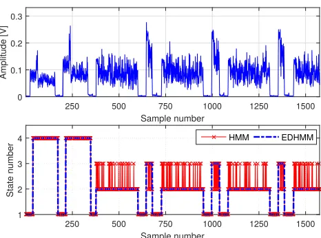
Fig. 6 shows a trace decoding example for our diagnosis tool. In the upper part of the figure, we show the raw trace as captured by the Sivers IMA converter. The two initial frames are beacons that indicate the start of a data burst. After that, we observe a sequence of data and acknowledgment frames (c.f. Fig. 1). The lower part of the figure shows that our framework can correctly identify all frames in the trace. We observe that the framework successfully classifies data packets, acknowledgments, beacons, and inter-frame spacing. Moreover, Fig. 6 also demonstrates the need for our EDHMM approach. The HMM method wrongly classifies many of the samples—within a data or acknowledgment frame, it often fluctuates between states. In contrast, the EDHMM classifies all samples correctly, even in case of varying data packet lengths (not shown in Fig. 6 due to space constraints).

250 500 750 1000 1250 1500

Sample number 0

0.1 0.2 0.3

Amplitude [V]

250 500 750 1000 1250 1500

Sample number 1

2 3 4

State number

HMM EDHMM

Fig. 6. Trace decoding example for our machine learning framework.

no blockage

0 0.5 1

Time [s] 0

20 40 60 80

DATA counter [

×

1000] SN1 SN₂

hard blockage

0 2 4

Time [s] SN₁

SN₂

soft blockage

0 1 2

Time [s] SN₁

SN₂

0 0.5 1

Time [s] 0

1 2 3 4

CTRL counter [

×

1000] SN1 SN₂

0 2 4

Time [s] SN₁

SN₂

0 1 2

Time [s] SN₁

SN₂

Fig. 7. Number of data and control packets identified by our tool. We show the results for two sniffers SN1 and SN2 placed at different locations.

In addition to the visual inspection in Fig. 6, we validate our framework using two approaches. First, we compare the number of data packets that our tool identifies with the number of packets that the driver of our 60 GHz device reports. For the case without blockage in Fig. 7, the driver reports31960

sent packets at the end of the trace. This matches the data packet counter in our results. Second, we record the same data exchange using two independent sniffers SN1 and SN2,

and process the resulting traces using our framework. For no blockage, Fig. 7 shows that both sniffers count the same number of both data and control packets. This again validates that our framework is correctly decoding the trace. For data packets, the counter stabilizes at one second at which point we stop the data transmission. Still, the control packet counter increases steadily because the devices continue to exchange control packets even if no data transmission is taking place.

burst length

0.5 1 1.5 2

Time [ms]

Link 1: MCS = 11, BP_A Link 2: MCS = 11, BP_B Link 3: MCS = 8, BP_B

DATA length

5 10 15 20 25

Time [µs] 0

0.2 0.4 0.6 0.8 1

ECDF

Link 1: MCS = 11, BP_A Link 2: MCS = 11, BP_B Link 3: MCS = 8, BP_B

Fig. 8. CDF of packet and burst lengths for three links deployed in the same environment but with varying performance. “BP” stands for beampattern.

blockage”, which refers to partial blockage such as waiving a hand in the boresight of the antenna.

B. Regular Operation

Next, we show some selected diagnosis capabilities of our tool for regular link operation. Fig. 8 depicts the Empirical Cumulative Distribution Function (ECDF) of the packet and burst lengths that our tool computes for different links. All links have the same length and are deployed in the same location. However, we change their orientation to induce different antenna beam patterns which result in suboptimal per-formance, and which our framework can identify. The protocol used by our 60 GHz test devices defines that the maximum burst length is two milliseconds and the maximum aggregated packet length is 20 microseconds. Since we perform this experiment with full transmission buffer at the nodes, the burst and packet lengths should match the maximum values.

For Link 1 in Fig. 8, we observe that the packet lengths do not match the maximum size. While the burst lengths are as expected, the significant fraction of short packets shows that Link 1 is not operating properly. Indeed, our framework also reveals that the trace energy level differs compared to Link 2, which suggests antenna misalignment. We omit the energy trace level in the interest of space but the device driver reveals that both Links 1 and 2 operate otherwise identically in terms of MCS and traffic load. In other words, our framework successfully identifies the suboptimal device orientation for Link 1. Fig. 8 shows that Link 3 performs even better in terms of packet length. Again, the device driver confirms this insight since Link 3 uses a more robust MCS than Link 2. Thus, Link 3 is more likely to succeed when transmitting longer packets.

C. External Disturbance

Regarding external disturbances, we focus on the case of link blockage. Our tool is able to identify and classify such blockage. This provides means for network operators to determine how often blockage actually occurs for a certain mm-wave link during a certain time-frame, for instance, a day. Identifying blockage is challenging because it may block the LOS path to the sniffer, too. To prevent this, our framework can record and compare the channel activity from two or more sniffers at different locations, as shown in Fig. 9. We

1.929 1.930 1.931 1.932 1.933 Time [s]

0.0 0.1

Amplitude [V]

SN₁

1.929 1.930 1.931 1.932 1.933 Time [s]

0.0 0.1 0.2

Amplitude [V]

SN₂

Fig. 9. Blockage recorded from two different locations SN1 and SN2. The figure shows a fraction of the blockage, i.e., the blockage affects all samples.

1.5 1.6 1.7 1.8 1.9 2.0

Time [s] 0.0

0.1 0.2 0.3 0.4

Amplitude [V]

SN₁ BR location

1.5 1.6 1.7 1.8 1.9 2.0

Time [s] 0.0

0.1 0.2 0.3 0.4 0.5

Amplitude [V]

SN₂ BR location

Fig. 10. Beam refinement sequences during soft link blockage.

observe that while sniffer SN1 barely receives any of the

activity prior to second1.93, SN2 is able to receive all frames

during the blockage. This allows our framework to obtain a much more complete view of the activity on the channel. Based on this information, we automatically identify beam refinement (BR) sequences. Such sequences are rare in static scenarios but are likely to occur if the link is impaired. Fig. 10 depicts a segment of the trace in Fig. 9, overlapped with the locations at which our framework identifies BR sequences. We observe that the BRs identified by both sniffers match but that not all sniffers capture all sequences due to the blockage. This highlights again the benefit of being able to analyze the network behavior from multiple viewpoints. Moreover, Fig. 9 depicts a soft blockage. Thus, the connection does not break and the device continuously adapts its beampattern, resulting in a large number of BRs. In contrast, hard blockage results in less BRs since the transmitter and the receiver cannot communicate during the blockage. Table I shows the average number of BRs per trace for no blockage, soft blockage, and hard blockage. The difference in terms of BR frequency allows our diagnosis tool to classify blockage. This is highly valuable to determine why a mm-wave link is performing poorly.

TABLE I

BEAM REFINEMENT SEQUENCE FREQUENCY FOR BLOCKAGE SCENARIOS

No Blockage Hard Blockage Soft blockage

0 BRs/trace 0.42 BRs/trace 4.02 BRs/trace

as blockage occurs. The underlying reason is that one of the sniffers does not receive the full channel activity while the other one does. While not as unambiguous as the detection of BRs, this also hints at potential blockage scenarios. We observe that hard blockage causes a stronger disagreement than soft blockage, providing means to differentiate them. The mismatch among sniffers is less explicit for control packets since the shape of such patterns is easier to identify than the shape of data packets. Hence, both sniffers are more likely to correctly decode such control packets even in case of blockage.

IX. CONCLUSION

We use machine learning techniques to design, implement, and evaluate a diagnosis tool for IEEE 802.11ad networks. Our tool uses narrowband physical layer energy traces of one or more sniffers to identify lower-layer performance issues. Network planners, administrators, as well as researchers can use our tool to improve the performance of mm-wave networks even though COTS networking devices provide no access to lower-layer information. To address the non-stationarity of energy traces, we use sophisticated machine learning tools and dynamically update the parameters of our model. Moreover, we use a combination of template matching and an EDHMM to deal with the complex characteristics of the traces and the behavior of IEEE 802.11ad devices. As a result, we achieve an ideal trade-off between the efficient but limited monitoring capabilities of IEEE 802.11ad devices in monitor mode, and the highly detailed but costly decoding of full bandwidth signals using software-defined radios. Finally, we use practical COTS 60 GHz hardware to validate our tool and show that it correctly identifies lower-layer performance issues.

X. ACKNOWLEDGEMENTS

This work was supported in part by the European Research Council grant ERC CoG 617721, the Ramon y Cajal grant from the Spanish Ministry of Economy and Competitive-ness RYC-2012-10788, and the Madrid Regional Government through the TIGRE5-CM program (S2013/ICE-2919).

REFERENCES

[1] R. R. Choudhury and N. H. Vaidya, “Deafness: a MAC Problem in Ad Hoc Networks When Using Directional Antennas,” inProc. ICNP, 2004. [2] T. Nitsche, G. Bielsa, I. Tejado, A. Loch, and J. Widmer, “Boon and Bane of 60 GHz Networks: Practical Insights into Beamforming, Interference, and Frame Level Operation,” inProc. of CoNEXT’15, 2015. [3] Y. Zhu, Z. Zhang, Z. Marzi, C. Nelson, U. Madhow, B. Y. Zhao, and H. Zheng, “Demystifying 60GHz Outdoor Picocells,” inProc. of ACM Mobicom’14, 2014.

[4] S. K. Saha and D. Koutsonikolas, “Towards Multi-gigabit 60 GHz Indoor WLANs,” inProc. of IEEE ICNP’15, 2015.

[5] IEEE, “Wireless LAN Medium Access Control (MAC) and Physical Layer (PHY) Specifications Amendment 3: Enhancements for Very High Throughput in the 60 GHz Band,”IEEE Std 802.11ad-2012, 2012. [6] M. K. Haider and E. W. Knightly, “Mobility Resilience and Overhead

Constrained Adaptation in Directional 60 GHz WLANs: Protocol Design and System Implementation,” inProc. of ACM MobiHoc, 2016.

[7] S. Sur, X. Zhang, P. Ramanathan, and R. Chandra, “Beamspy: Enabling robust 60 ghz links under blockage,” inProc. of NSDI, 2016. [8] S. Sur, V. Venkateswaran, X. Zhang, and P. Ramanathan, “60 GHz

Indoor Networking Through Flexible Beams: A Link-Level Profiling,” inProc. of ACM SIGMETRICS’15, 2015.

[9] R. do Carmo and M. Hollick, “DogoIDS: A Mobile and Active Intrusion Detection System for IEEE 802.11s Wireless Mesh Networks,” inProc. of HotWiSec, 2013.

[10] D. S. Berger, F. Gringoli, N. Facchi, I. Martinovic, and J. Schmitt, “Gaining Insight on Friendly Jamming in a Real-world IEEE 802.11 Network,” inProc. of WiSec, 2014.

[11] T. T. T. Nguyen and G. Armitage, “A Survey of Techniques for Internet Traffic Classification Using Machine Learning,”IEEE Communications Surveys Tutorials, vol. 10, no. 4, 2008.

[12] A. McGregor, M. Hall, P. Lorier, and J. Brunskill, “Flow Clustering Using Machine Learning Techniques,” inProc. of PAM, 2004. [13] L. R. Rabiner, “Readings in Speech Recognition,” ch. A Tutorial on

Hid-den Markov Models and Selected Applications in Speech Recognition, Feb 1990.

[14] Y. Niu, Y. Li, D. Jin, L. Su, and A. V. Vasilakos, “A Survey of Millimeter Wave Communications (mmWave) for 5G: Opportunities and Challenges,”Wireless Networks, vol. 21, Nov 2015.

[15] A. P. Dempster, N. M. Laird, and D. B. Rubin, “Maximum Likelihood From Incomplete Data via the EM Algorithm,” Journal of the Royal Statistical Society, Series B, vol. 39, no. 1, 1977.

[16] L. E. Baum, T. Petrie, G. Soules, and N. Weiss, “A Maximization Tech-nique Occurring in the Statistical Analysis of Probabilistic Functions of Markov Chains,”Annals of Mathematical Statistics, vol. 41, Feb 1970. [17] L. E. Baum and J. A. Eagon, “An Inequality With Applications to Statistical Estimation for Probabilistic Functions of Markov Processes and to a Model for Ecology,”Bulletin of the American Mathematical Society, vol. 73, May 1967.

[18] L. E. Baum and G. R. Sell, “Growth Transformations for Functions on Manifolds,”Pacific Journal of Mathematics, vol. 27, no. 2, 1968. [19] D. Garcia, “Robust Smoothing of Gridded Data in One and Higher

Dimensions with Missing Values,” Computational Statistics & Data Analysis, vol. 54, Apr 2010.

[20] D. Garcia, “A Fast All-in-One Method for Automated Post-Processing of PIV Data,”Experiments in Fluids, vol. 50, Oct 2011.

[21] J. Lee Rodgers and W. A. Nicewander, “Thirteen ways to look at the correlation coefficient,”The American Statistician, vol. 42, Feb 1988. [22] T. Kailath and H. V. Poor, “Detection of Stochastic Processes,”IEEE

Transactions on Information Theory, vol. 44, Oct 1988.

[23] A. Mueen, H. Hamooni, and T. Estrada, “Time series join on subse-quence correlation,” inProc. of IEEE ICDM, Dec 2014.

[24] A. Mueen, E. Keogh, and N. Young, “Logical-shapelets: an expressive primitive for time series classification,” in Proc. of ACM SIGKDD international conference on Knowledge discovery and data mining, Aug 2011.

[25] IEEE, “Wireless LAN Medium Access Control (MAC) and Physical Layer (PHY) Specifications Amendment 3: Enhancements for Very High Throughput in the 60 GHz Band,”IEEE Std 802.11ad-2012, Dec 2012. [26] C. Bishop,Pattern Recognition and Machine Learning. Springer, 2007. [27] S. T. Roweis, “Constrained Hidden Markov Models,” inProc. of NIPS,

Nov 1999.

[28] J. MacQueen, “Some Methods for Classification and Analysis of Multi-variate Observations,” inProc. of Berkeley Symposium on Mathematical Statistics and Probability, 1967.

[29] D. Arthur and S. Vassilvitskii, “K-means++: The Advantages of Careful Seeding,” inProc. of SODA, Jan 2007.

[30] S. E. Levinson, “Continuously Variable Duration Hidden Markov Mod-els for Automatic Speech Recognition,” Computer Speech and Lan-guage, vol. 1, Mar 1986.

[31] C. Mitchell and L. Jamieson, “Modeling Duration in a Hidden Markov Model with the Exponential Family,” inProc. in ICASSP, Apr 1993. [32] S.-Z. Yu and H. Kobayashi, “An Efficient Forward-Backward Algorithm

for an Explicit-Duration Hidden Markov Model,”IEEE Signal Process-ing Letters, vol. 10, Jan 2003.

[33] S.-Z. Yu and H. Kobayashi, “Practical Implementation of an Efficient Forward-Backward Algorithm for an Explicit-Duration Hidden Markov Model,”IEEE Transactions on Signal Processing, vol. 54, May 2006. [34] S.-Z. Yu, “Hidden Semi-Markov Models,” Artificial Intelligence,