FLOW AROUND BLUFF BODIES WITH CORNER MODIFICATIONS ON CROSS-SECTIONS

(1)

BY

RUJUN LIU

BE, Power Engineering of Aircraft, Nanjing University of Aeronautics and Astronautics, China, 2017

THESIS

Submitted to the University of New Hampshire in Partial Fulfillment of

the Requirements for the Degree of

Master of Science

in

Mechanical Engineering

(2)

(3)

This thesis has been examined and approved in partial fulfillment of the requirements for the degree of Master of Science in Mechanical Engineering by:

Thesis Director, Dr. Christopher White, Professor of Mechanical Engineering

Dr. Alireza Ebadi,

Lecturer of Mechanical Engineering

Dr. Ivaylo Nedyalkov,

Lecturer of Mechanical Engineering

on 07/26/2019.

(4)

(5)

ACKNOWLEDGMENTS

I would like to thank my advisor, Christopher White, Professor at the University of New

Hamp-shire, who provided many suggestions on my graduate study and this thesis. I would like to thank

Alireza Ebadi, lecturer at the University of New Hampshire, who helped me with the wind tunnel

experiment. I would like to thank Zhijing Xu, Visiting Scholar at the University of New

Hamp-shire, who provided guidance for the numerical simulation.

I would like to thank my parents, Shuxiang Liu and Jie Zhou, whose financial and emotional

support enabled me to pursue knowledge in the United States, seven thousand miles away from my

home. I would like to thank my future employer, AECC Commercial Aircraft Engine Co. Ltd., for

offering me a job in Shanghai a few months ago, which enabled me to devote all my attention to

writing this thesis without distraction.

I would like to thank Editage (www.editage.com) for English language editing.

Finally, I would like to thank my girlfriend, Shan Cheng, MS at the University of Texas, Austin,

who comforted and accompanied me with patience, and provided me with the energy, motivation,

(6)

NOMENCLATURE

Roman Symbols

A Area

Cd Drag Coefficient

D Diameter / Side Length of Cylinder

E Mechanical Energy

F Force

f Vortex Shedding Frequency

Fd Drag Force

g Gravity Acceleration

H Height of Wind Tunnel / Height of Computational Domain

h Water Head Height

L Length of Cylinder / Length of Computational Domain

Lw Length of Föppl Vortices

M a Mach Number

p Pressure

P r Prandtl Number

Q Total Energy

q Internal Energy

r Corner Radius

Re Reynolds Number

St Strouhal Number

t Time

(10)

u Velocity onxDirection

V Volume

v Velocity onyDirection

W Power Output

w Velocity onz Direction

Greek Symbols

λ Volume Viscocity

µ Fluid Viscocity

ρ Fluid Density

τ Surface Shear Force

ξ Grid Quantity

Abbreviations

AMG Method Algebraic Multigrid Method

ASM Algebraic Stress Model

BEM Boundary Element Method

CFD Computational Fluid Dynamics

ELD Engineering Laboratory Design

EVM Eddy Viscosity Model

FDM Finite Difference Method

FEM Finite Element Method

FVM Finite Volume Method

LDA Laser Doppler Anemometry

LES Large Eddy Simulation

PDE Partial Differential Equation

SST Model Menter’s Shear Stress Transport Turbulence Model

(11)

LIST OF TABLES

Table Page

1.1 Results of Delany’s Experiment (1953) . . . 7

3.1 Computational Domain Study . . . 31

3.2 Grid Type Study . . . 32

5.1 Scaled Reattachment Length Comparison . . . 41

5.2 Strouhal Number Comparison . . . 45

5.3 Drag Coefficient Comparison . . . 46

B.1 Original Data from Wind Tunnel Experiment . . . 87

B.2 Experiment Result . . . 87

B.3 Density of Water . . . 88

(12)

LIST OF FIGURES

Figure Page

1.1 Bluff Body Application Example: I-Beam . . . 2

1.2 Comparison ofCdbetween Different Corner Radius Ratios . . . 8

2.1 Flow Structure When Passing Through a Cylinder . . . 22

3.1 Cross-Sections of CylindersC1toC5 (From Left to Right) . . . 26

3.2 Flow Diagram of CFD Simulation . . . 28

3.3 Schematic Diagram of Computational Domain . . . 30

3.4 Computational Domain Comparison . . . 31

3.5 Grid Type Comparison . . . 33

4.1 Sketch Map of Wind Tunnel for Experiment . . . 35

4.2 Assembly Drawing of Wind Tunnel for Experiment . . . 35

5.1 Simulation Validation Examination – Drag Coefficient Comparison . . . 41

5.2 Scaled Reattachment Length VS Reynolds Number . . . 42

5.3 Scaled Reattachment Length VS Corner Radius Ratio . . . 43

5.4 Strouhal Number VS Reynolds Number . . . 44

5.5 Strouhal Number VS Corner Radius Ratio . . . 45

5.6 Drag Coefficient VS Reynolds Number . . . 47

5.7 Drag Coefficient VS Corner Radius Ratio . . . 48

(13)

5.9 Experiment Result – Drag Coefficient VS Corner Radius Ratio . . . 50

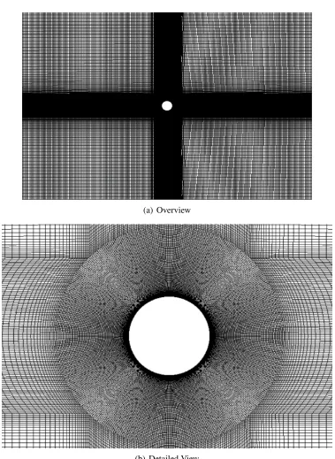
5.10 Three Dimensional Simulation – Overview . . . 51

5.11 Three Dimensional Simulation – Detailed View . . . 51

5.12 Error Analysis – Cylinder Length . . . 52

A.1 H-Type Grid . . . 60

A.2 O-Type Grid . . . 61

A.3 C-Type Grid . . . 62

A.4 Mesh of25D×20D. . . 63

A.5 Mesh of30D×20D. . . 64

A.6 Mesh of50D×20D. . . 65

A.7 Final Mesh Generation of Cylinders . . . 66

A.8 Flow Structures ofC1– Steady Flow . . . 67

A.9 Flow Structures ofC1– Unsteady Flow . . . 68

A.10 Streamlines of Flow ofC1– Steady Flow . . . 69

A.11 Streamlines of Flow ofC1– Unsteady Flow . . . 70

(14)

(15)

ABSTRACT

Flow around Bluff Bodies with Corner Modifications on Cross-Sections

by

Rujun Liu

University of New Hampshire, September, 2019

This research aims to illustrate how the flow around a cylinder changes when the cylinder’s

cross-section is systematically changed from square to circle by modifying the corner radius.

Numerous research studies have been performed on the flow around circular cylinders and

square cylinders leading to a relatively complete understanding of them. In the early 20th century,

von Kármán and Rubach described the theoretical basis and provided an analytical solution to the

flow around circular cylinders at low Reynolds number. Later, experiments on the flow around

square cylinders were conducted by Nakaguchi, Bearman, and other researchers. However, until

now, only a few researchers have focused on how the flow structure evolves when the cylinder’s

cross-section gradually changes from a square to a circle by increasing the radius of the corner

edges.

In this study, five numerical simulations were conducted. Each simulation performed

calcula-tions on a cylinder model where the shape was changed systematically from a square to a circle.C1

is a square cylinder with a side length ofD= 0.375inches andr/D= 0whereris the radius of the corner edge;C2 toC4denote three rounded-corner square cylinders with the same side length

Dandr/Dratios of0.167,0.247, and0.333, respectively.C5is a circular cylinder with a diameter

of0.375inches (r/D= 0.5). Simulations were performed in two dimensions at Reynolds number of 10 to 200, using the control volume technique and Gauss-Siedel iterative method in conjunction

with the Algebraic Multigrid (AMG) solver in ANSYS FLUENT 18.2.

The simulated flow around the cylinders was illustrated by planar contours of various flow

variables (e.g., velocity and pressure). The evolution of the flow behavior when transitioning from

a square cylinder to a round cylinder are described by comparing the scaled reattachment length,

(16)

of the Reynolds number, the drag coefficient and scaled reattachment length decrease, while the

Strouhal number increases when a cylinder changes from a square shape into a circular shape.

However, under specific conditions, the drag coefficient of a rounded-corner square cylinder may

be lower than that of a circular cylinder with the same dimension.

In addition, a series of experiments were performed to study the flow around the described set

of cylinders above at higher Reynolds number ranging from approximately4400 to 16000. The

experiments were performed in an Engineering Laboratory Design (ELD) Model 404 wind tunnel

located in Kingsbury Hall at the University of New Hampshire. The test-section dimensions are

18 inches x 18 inches cross-section and 36 inches in length with a maximum speed of 150 mph.

The cylinders were centered in the test-section with the cylinder length perpendicular to the flow

direction. The aerodynamic drag on a cylinder was measured as a function of wind speed in the

tunnel using a TecQuipment AFA2 lift/drag force balance. The wind speed in the test section was

measured using a Pitot-static tube connected to a differential pressure transducer. The trends of

drag coefficient observed in the experiments are similar to those observed in the simulations.

(17)

CHAPTER 1 INTRODUCTION

1.1 Background and Significance of This Study

Fluid flows occur in a wide range of natural phenomena and engineering applications and their

dy-namics depend solely on their boundary conditions and initial conditions. In many of these flows,

the dynamics are so complex that their understanding requires the development and

implementa-tion of flow models. The modeling of fluid flows incorporates parameters and variables such as

fluid state (liquid or gas), physical characteristics of the fluid (viscosity, compressibility, thermal

conductivity, etc.), fluid variables (temperature, velocity, etc.), and external conditions (boundary

and initial conditions) [23].

Depending on the situation, a flow is generally classified as either laminar flow or turbulent

flow. Turbulent flows are inherently large Reynolds number flows, Re = U L/ν, where U and

L are characteristic velocity and length scale of the flow, andν is the kinematic viscosity of the fluid. The critical Reynolds number Recr denotes the transition between a laminar flow and a turbulent flow. Specifically, a flow will be laminar if Re < Recr and turbulent if Re > Recr. In laminar flow, the fluid particles move along smooth streamlines, while in turbulent flow, they

move along random curved lines. Turbulent flow is dominant in the natural environment and in

most engineering applications. Owing to its complex and seemingly random motions, it is not

possible to derive analytical solutions of turbulent flows. As such, turbulence is considered the

most important unsolved problem in classical physics.

Bluff bodies, also called blunt bodies in some research papers, are the geometries of structures

with a non-streamlined cross-section in which the flow will separate from the surface boundary

(18)

on the body due to viscous effects [4] [21]. The total drag of an object can be decomposed into

pressure drag (form drag), frictional drag (viscous drag) and for lifting bodies induced drag. A

body dominated by pressure drag is called a bluff body, while a body dominated by frictional

drag is called a streamlined body. Bluff bodies include a wide variety of geometric shapes, e.g.,

cylinders, cuboids, spheres, and pyramids. Some of the geometries are widely used in engineering

and industry, especially cuboids and cylinders.

It is important to study the flow around bluff bodies because most vehicles, structures, and

projectiles are shaped as bluff bodies. The flow around a bluff body imparts a force that can lead to

increased fuel consumption (and subsequent increased emissions), mechanical wear, and potential

catastrophic failure. In 1940, Tacoma Narrows Bridge in the U.S. state of Washington collapsed

due to the resonance between Kármán Vortex Street shedding frequency and the natural frequency

of the bridge [2]. Meanwhile, by studying the flow around bluff bodies of different structures, it is

possible to obtain information such as the position of transition point and the wake strength under

different conditions. By changing the shape of bluff bodies, it is possible to better understand flow

separation and strategies to prevent or minimize the effects of flow separation.

Figure 1.1.Bluff Body Application Example: I-Beam

In civil construction, most building structures have rectangular or circular cross-sections. A

sit-uation of wind passing around this kind of structure can be simplified into a model of flow around

(19)

cross-sections. There has been considerable research on the 2D flow around both a square and a

circle, but only a few papers have discussed how the flow structure changes when the geometry

shape gradually changes from square to circle, by increasing the radius of the rounded corner of

the square. Rounded-corner squares are advantageous because they may result in a better

aero-dynamic performance than both squares and circles, in terms of boundary layer separation, wake

length, drag force, and vortex street. Also, they are easier to manufacture and require a lower cost

compared with streamlined bodies. The present study mainly focuses on this point, by using the

computational fluid dynamics (CFD) method and wind tunnel experiment.

1.2 Former Research Results on Flow around Bluff Bodies

Beginning with the origins of modern fluid dynamics in the late 1800’s, the topic of flow around

bluff bodies has always received considerable attention from researchers [54]. Corresponding to

the subject of this paper, the status of three aspects of this research are discussed: the flow around

a cylinder (circular cylinder), the flow around a cuboid (square cylinder), and the flow around a

rounded-corner square cylinder.

1.2.1 Research on Flow around a Circular Cylinder

In 1912, von Kármán [19] first described the characteristics of flow around a circular cylinder,

including the formation of the vortex street and the relationship between vortex momentum and

wake resistance, which was a milestone in the research on flow around a cylinder. In 1913, Ludwig

Föppl [12] introduced a pair of vortices appearing behind a cylinder in a steady flow under a low

Reynolds number.

Later on, many experiments were performed on this topic. Taneda [48] [49] described the

for-mation of Föppl’s vortices behind a cylinder at Re=5. He also stated that Föppl’s vortices attached

behind a cylinder but were stretched when Re < 45. IfRe > 45, the vortex becomes asymmet-ric and oscillates, ultimately separating from the cylinder and evolving into the Kármán vortex

street. In 1954, Rushko [42] studied the wake development downstream of a circular cylinder for

(20)

Reynolds number was varied.Re= 40to150is the stable range, where the flow is mainly regular and has a periodic vortex without any turbulence. Re= 150to300is the transition range, where the turbulence is initiated by laminar-turbulent transition. Re > 300is the irregular range, which is dominated by turbulent velocity fluctuation. Mathis [25] experimentally proved the idea of three

different flow patterns raised by Roshko. Williamson [53] studied the three-dimensional transition

of the flow behind a circular cylinder and found the formation of a three-dimensional shedding

vortex, whose transition begins when the Reynolds number increases from180to260.

The involvement of laser technology brought increasing accuracy and efficiency to the

exper-iments. Provansal [38] investigated the wake of a circular cylinder near the oscillation

thresh-old using a laser probe. Perrin [33] analyzed the turbulence properties in unsteady flows around

circular cylinder wakes with a low aspect ratio (L/D = 4.8) and a high blockage coefficient (D/H = 0.208) by using PIV, with similar conditions as that in this paper. Price [37] performed an experiment on flow visualization around a circular cylinder near a plane wall for Reynolds

num-bers between1200and4960, by changing the diameter of the cylinder. The results were classified

into four different flow patterns according to the distance between the cylinder and the plane wall.

In 2008, Parnaudeau [31] studied the flow structure over a circular cylinder atRe= 3900, which is the boundary between laminar flow and turbulent flow. The study was based on hot-wire

anemom-etry and PIV, and focused on the turbulence statistics and power spectra near the wake up to ten

diameters.

By the 1960s, with the development of computer technology, CFD technology became a hot

topic in fluid research. With lesser cost and simpler facilities, it was possible for researchers to

obtain the results of complicated flow fields, the experiments of which are difficult to perform. This

resulted in a rapid growth of fluid dynamics research leading to fruitful discoveries. Rahman [39]

investigated the flow around a circular cylinder using the 2-D finite volume method, at Reynolds

numbers of1000 and3900. He compared the lift and drag coefficients of the cylinder calculated

(21)

vibrations in three dimensions using a large eddy simulation (LES) Smagorinsky model. The

simulation result matched the experimental results obtained under similar conditions by Achenbach

[1] in 1968. Rajani [40] focused on the analysis of two- and three-dimensional flow past a circular

cylinder in different laminar flow regimes with an implicit pressure-based finite volume method

and measured the mean surface pressure, skin friction coefficients, and the size and strength of

the recirculating wake for the steady flow regime as well as for the Strouhal frequency of vortex

shedding.

1.2.2 Research on Flow around a Square Cylinder

Studies on the flow around a square cylinder originated from the studies on the flow around

other bluff bodies, including flat plates, wedges, cuboids, and other bodies with similar

geome-tries. In 1955, Rushko [43] first compared the wake Strouhal number and the drag coefficient of

a circular cylinder, a flat plate, and a90◦ wedge under different base pressure coefficients.

Nak-aguchi [29] carried out an experiment on the drag force of flow around rectangular cylinders, which

revealed that the drag coefficient is related to the ratio between the rectangle’s side length parallel

to the flow direction and perpendicular to the flow direction. Bearman’s [3] research confirmed

Nakaguchi’s findings and presented further details of the flow structure including the base pressure

coefficient, drag coefficient, and Strouhal number. Castro and Robins [5] considered the effect of

changes in block shape on the flow structure, including modification of the cube height and

an-gle towards flow direction. In 1982, Hunt [16] simulated the atmosphere structure and generated

pressure and velocity fields on the surface of a square cylinder. It was found that under boundary

layer simulations with scales of1/180and 1/360, the influence of roughness of cylinder surface increases when the Reynolds number increases. Meanwhile, Hunt discovered that negative peaks

of pressure occurred on the front surface, which had been ignored by Castro and Robins.

Martin-uzzi and Tropea [24] introduced the flow visualization technique to the study of square cylinders,

e.g., crystal violet, oil-film, and laser-sheet. It was investigated whether the vortex exists on all

(22)

foundation for further research. Later on, Hussein and Martinuzzi [17] performed experiments

on the three-dimensional flow around a surface mounted cube in a channel by using laser doppler

anemometry (LDA) measurement. The production, convection, and transport of the turbulence

kinetic energy in the obstacle wake were obtained. Simultaneously, the turbulence dissipation rate

was obtained to closely balance the K-transport equation. By using PIV technology, Ito and his

team [18] performed an experiment to clarify the characteristics of spatial flow structures and wind

pressures above the top surface of a cube, and found that a flat conical vortex was formed when

the intensity of turbulence of the approaching flow was large.

Similar to the flow around circular cylinders, numerical simulation has played a significant role

in modern research. Baetke and his colleagues [47] presented the simulation result of turbulent

flow around a surface-mounted cube and over a surface-mounted square rib. For the first case, the

standardK − turbulence model was introduced together with Reynolds equations. The second case was solved by applying the concept of large-eddy simulation. Murakami [28] [27] focused

on the improvement of the turbulence model. The K − Eddy Viscosity Model (K − EVM), Algebraic Stress Model (ASM), and LES were examined for accuracy, and it was found that LES

had the best agreement with the results of the tunnel test on the flow around a cube. Sohankar et

al. [47] calculated the 2-D flow around a square cylinder at incidence between0◦and45◦ for a low

Reynolds number of 45to200, and the flow was presumably laminar. Richards and Hoxey [41]

calculated the constants in theK−and boundary conditions for atmospheric wind engineering problems based on the measurement results obtained from Silsoe Research Institute.

1.2.3 Research on Corner Modification

Besides the studies on circular cylinder and square cylinder, some researchers focused on the

corner modification of a square cylinder. The flow structure around a circular and square cylinder

is so different that it made people curious about the changes in flow structure when the shape of

(23)

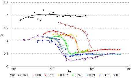
gradually increases from0 to half of the side length (r/D = 0.5), which makes the geometry a circle with a diameter ofD.

In 1953, Delany and Sorensen [8] measured the drag forceFdand drag coefficientCdof squares with corner radius modification. The results were measured in the Ames 7- by 10-foot wind tunnel.

It was concluded by Delany that Cd decreased with increase in the corner radius ratio in most geometries. A part of the data and the results of the flow around rounded-corner squares are

provided in Table 1.1.

D∗ r∗ Corner Radius Ratio (r/D) Re Cd 12 0.25 0.021 1×105 2.0 4 0.08 0.021 1×105 ₂_.₀

1 0.02 0.021 1×105 2.0 12 2.00 0.167 2×105 1.2 12 4.00 0.333 1×105 ₁_.₀

1 0.33 0.333 1×105 ₁_.₀

∗: In Inches

Table 1.1.Results of Delany’s Experiment (1953)

Later, in 1958, Polhamus [34] performed experiments on cylinders with similar shapes in the

Langley 300-MPH 7- by 10-foot tunnel. Two rounded-corner square cylinders withr/D = 0.245 and0.080were tested underRe = 2.5×105 to approximately1.8×106. It was found thatCdof a square withr/D= 0.245has a rapid decrease atRe= 4×105, but only a gentle decrease over

Re= 1×106_{in the case of}_r/D_{= 0}_._080.

Hu et al. [15] studied this topic using PIV, LDA, and hotwire measurements. Four bluff

bod-ies of r/D equal to 0(square cylinder), 0.157, 0.236, and 0.5 (circular cylinder) were examined respectively atRe= 2600and6000. It was found that asr/Dincreases from0to0.5, the maxi-mum strength of the shed vortices attenuates, the circulation associated with the vortices decreases

progressively by 50%, the Strouhal number,St, increases by about 60%, the convection velocity of the vortices increases along with the widening of the wake width by about25%, and the vortex

(24)

Hinsberg et al. [51] performed experiments on cylinders with rounded corners ofr/D = 0.16 and r/D = 0.29. A comparison was made between the results of their research and those of previous researches, including the researches of:

1. Delany and Sorensen [8]:r/D= 0.021;r/D= 0.167;r/D = 0.333;

2. Polhamus [34]: r/D= 0.08;r/D= 0.245;

3. Schewe [44]:r/D= 0.5(Circular Cylinder);

Figure 1.2. Comparison ofCdbetween Different Corner Radius Ratios

Figure 1.2 shows the comparison between the results obtained by Hinsberg et al. and those of

the studies listed above. The colors were set as spectrum gradient according to ther/Dratio, and trendlines were added to clearly indicate the relationship between the corner radius ratio and drag

(25)

1.3 Objective and Main content of This Study

This study mainly focuses on the flow around square cylinders with corner modifications under

low Reynolds numbers of 10to 200, which have not been focused on by many researchers, and

seeks to figure out the changes in flow structure due to the corner effect in flow regimes of the

laminar range. Meanwhile, the study of flow around the same cylinders under medium Reynolds

numbers from around4300to16600was conducted to compare with former researches and verify

the other results.

A total of five cylinder models are introduced, with the shape gradually changing from a square

to a circle. C1 is a square cylinder with a side length of0.375inch, i.e., r/D = 0. C2 toC4 are

three rounded-corner square cylinders with the same side length and r/D ratio of 0.167, 0.247, and0.333. C5 is a circular cylinder with a diameter of0.375inch (r/D= 0.5).

Due to the computational capability of the present condition, as well as the dimension and

velocity range of the wind tunnel, the result of low Reynolds number is obtained through numerical

simulation, and that of medium Reynolds number is obtained through a wind tunnel experiment.

Simulations were performed in two dimensions, using the control volume technique and

Gauss-Siedel iterative method in conjunction with the Algebraic Multigrid (AMG) solver in ANSYS

FLUENT 18.2. H-, O-, and C-types of structured grids were tested and compared. H-type grids

were chosen for the simulation. For the boundary conditions, the left wall was set as the flow

inlet and the right wall was set as the pressure outlet. All four wall boundaries were set as slip

walls, while the cylinder boundary was set as a non-slip wall to make sure that there is no relative

movement. The mesh independence was also taken into consideration. The calculation domain

was chosen for a dimension of30D×20Dand mesh quantity of around100,000. The data of drag coefficient, Strouhal number, and scaled reattachment length were collected for analysis.

Experiments were performed in an Engineering Laboratory Design (ELD) Model 404 wind

tunnel located in Kingsbury Hall at the University of New Hampshire. The test-section dimensions

(26)

(27)

CHAPTER 2 FUNDAMENTAL THEORY

2.1 Governing Equations

The flow around bluff bodies is a classic topic in fluid dynamics. To clearly illustrate and deeply

understand the flow structure, it is necessary to begin with the governing equations, which can be

derived from Newton’s first, second, and third laws, regarding conservation of mass, momentum,

and energy. The governing equations include the continuity equation, the momentum equation, the

energy equation, the Navier-Stokes equation, and Bernoulli’s equation [22].

2.1.1 The Continuity Equation

From the conservation of mass and Reynolds Transport Theorem, it is known that the mass

flow rate of the control volume is equal to the mass flow rate of the control surface, according to

the following equation:

D Dt

Z

V

ρdV = ∂

∂t

Z

V

ρdV + I

A

ρ ~UdA~ = 0 (2.1)

where t is the time,ρis the fluid density,U~ is the flow velocity,V is the control volume, andA~

is the control surface area.

According to the Gauss divergence theorem,

Z

V

∇ ·(ρ ~U)dV = I

A

ρ ~UdA~ (2.2)

(28)

∂ ∂t

Z

V

ρdV + Z

V

∇ ·(ρ ~U)dV = 0 (2.3)

Taking the derivative ofdV,

∂ρ

∂t +∇ ·(ρ ~U) = 0 (2.4)

Due to the low speed condition of the present study, the flow can be considered to be

incom-pressible, whereρ=const.and∂ρ/∂t= 0. Then, the Hamiltonian operator (∇) is expanded:

∂u ∂x +

∂v ∂y +

∂w

∂z = 0 (2.5)

This is the differential form of the continuity equation for incompressible flow, whereu,v, and

ware the velocities in thex,y, andzdirection.

If we apply ρ = const. and ∂ρ/∂t = 0 to Equation 2.1, the integral form of the continuity equation for incompressible flow can be obtained as follows:

I

A

~

UdA~ = 0 (2.6)

2.1.2 The Momentum Equation

The momentum equation is the application of Newton’s second law in fluid dynamics. If a

control volume is considered instead of a single particle, Newton’s second law can be written as

follows:

~ Fnet =

d dt

Z

V

ρ ~UdV (2.7)

whereF~netrepresents the externally applied forces.

On applying Reynolds transport theorem into Equation 2.7, we get

~ Fnet =

∂ ∂t

Z

V

ρ ~UdV + I

A

(29)

The momentum equation can also be written in the derivative form as follows:

∂(ρ ~U)

∂t =−∇p− ∇(ρ ~U) ~

U − ∇τ+ρF (2.9)

where pis the pressure, τ is the shear force on every surface, and F is the body force of the control volume.

If we expand all the Hamiltonian operators in Equation 2.9, we get

ρ∂u ∂t =−

∂p ∂x −(ρu

∂u ∂x +ρv

∂u ∂y +ρw

∂u ∂z)−(

∂ ∂xτxx+

∂ ∂yτyx+

∂

∂zτzx) +ρFx ρ∂v

∂t =− ∂p ∂y −(ρu

∂v ∂x +ρv

∂v ∂y +ρw

∂v ∂z)−(

∂ ∂xτxy +

∂ ∂yτyy+

∂

∂zτzy) +ρFy ρ∂w

∂t =− ∂p ∂z −(ρu

∂w ∂x +ρv

∂w ∂y +ρw

∂w ∂z)−(

∂ ∂xτxz+

∂ ∂yτyz+

∂

∂zτzz) +ρFz

(2.10)

These are the derivative forms of the momentum equation.

2.1.3 The Energy Equation

The energy equation shows the principle of the first law of thermodynamics on fluid dynamics.

It illustrates that the heat received by the control volume per unit time is equal to the sum of the

flow rate of the total energy and the power output by the control volume, i.e.,

Q= dE

dt +W (2.11)

whereQis the total energy received by the control volume per unit time,E is the flow rate of the mechanical energy, andW is the power output by the control volume.

For a control volume of a small amount of fluid, the mechanical energy includes the kinetic

energy and internal energy. The kinetic energy per unit mass is U~2_/₂ _{and the internal energy is}

(30)

dE

dt =

d dt

Z

V

ρ(q+U~

2

2 )dV (2.12)

On substituting Equation 2.12 and applying the Reynolds transport theorem into Equation 2.11,

we get

Q= ∂

∂t

Z

V

ρ(q+

~ U2

2 )dV + I

A (q+

~ U2

2 )(ρ ~U ·d

~

A) +W (2.13)

This is the energy equation in fluid dynamics.

2.1.4 The Navier-Stokes Equation

Stokes made a well-known hypothesis for Newtonian fluids (viscosity is a constant, i.e. µ =

const), which is as follows:

τxx =−p+ 2µ

∂u

∂x +λ∇ ·U~ τyy =−p+ 2µ

∂v

∂y +λ∇ · ~ U

τzz =−p+ 2µ

∂w

∂z +λ∇ · ~ U

τxy =τyx=µ(

∂u ∂y +

∂v ∂x) τxz =τzx=µ(

∂u ∂z +

∂w ∂x) τyz=τzy =µ(

∂v ∂z +

∂w ∂y)

(2.14)

whereλis the volume viscosity, which is usually equal to−2µ/3.

For the present research, we can apply the incompressible flow condition and substitute

Equa-tion 2.5 and EquaEqua-tion 2.10 into EquaEqua-tion 2.14. Then, we can obtain the Navier-Stokes equaEqua-tion for

(31)

ρ(∂u

∂t +u ∂u ∂x +v

∂u ∂y +w

∂u

∂z) = ρFx− ∂p ∂x +µ(

∂2u ∂2_x +

∂2u ∂2_y +

∂2u ∂2_z)

ρ(∂v

∂t +u ∂v ∂x +v

∂v ∂y +w

∂v

∂z) = ρFy − ∂p ∂y +µ(

∂2v ∂2_x +

∂2v ∂2_y +

∂2v ∂2_z)

ρ(∂w

∂t +u ∂w

∂x +v ∂w

∂y +w ∂w

∂z) = ρFz− ∂p ∂z +µ(

∂2_w

∂2_x +

∂2_w

∂2_y +

∂2_w

∂2_z)

(2.15)

This is the Navier-Stokes equation. It can also be rewritten using the Hamiltonian operator:

ρD ~ U

Dt =ρF − ∇p+µ∇

2_~

U (2.16)

2.1.5 The Bernoulli’s Equation

Navier-Stokes equation can be used to describe most types of flow; however, due to the

non-linear diffusion term, it is unable to derive an analytical solution using current mathematical

knowl-edge. However, for some special circumstances of flow, the equation of motion can be simplified

to a form without non-linear terms, which results in Bernoulli’s equation. It should be noted that

we only consider Bernoulli’s equation for incompressible flow in this paper.

To satisfy the requirements of Bernoulli’s equation, the flow must meet the following

charac-teristics:

1. Steady flow: The entire system must not change with time;

2. Incompressible flow: The density of fluid must be a constant. For gas, the Mach numberM a

should be less than0.3;

3. Frictionless flow: The friction due to viscous forces must be negligible;

4. Flow along a streamline: The fluid element must move along a streamline. Different

stream-lines must not intersect with each other.

Considering a system that satisfies the above requirements, the following equations must hold

(32)

∂u ∂y = ∂v ∂x, ∂u ∂z = ∂w ∂x, ∂v ∂z = ∂w ∂y ∂u ∂t = ∂v ∂t = ∂w

∂t =τ = 0

(2.17)

Substitute Equation 2.17 into Equation 2.10 and multiply dx, dy, and dz respectively to the first, second, and third equations:

0 =−∂p

∂xdx−(ρu ∂u

∂xdx+ρv ∂u

∂ydx+ρw ∂u

∂zdx) +ρFxdx

0 =−∂p

∂ydy−(ρu ∂v

∂xdy+ρv ∂v

∂ydy+ρw ∂v

∂zdy) +ρFydy

0 =−∂p

∂zdz−(ρu ∂w

∂xdz+ρv ∂w

∂ydz+ρw ∂w

∂zdz) +ρFzdz

(2.18)

Note that in Equation 2.17, ∂u/∂y = ∂v/∂x is equivalent to udy = vdx. Similarly, udz =

wdx,vdz =wdy. On applying this to Equation 2.18, we get

0 =−∂p

∂xdx−ρu( ∂u ∂xdx+

∂u ∂ydy+

∂u

∂zdz) +ρFxdx

0 =−∂p

∂ydy−ρv( ∂v ∂xdx+

∂v ∂ydy+

∂v

∂zdz) +ρFydy

0 =−∂p

∂zdz−ρw( ∂w

∂xdx+ ∂w

∂ydy+ ∂w

∂zdz) +ρFzdz

(2.19)

(33)

(∂p

∂xdx+ ∂p ∂ydy+

∂p ∂zdz)

+ρ[u(∂u

∂xdx+ ∂u ∂ydy+

∂u ∂zdz)

+v(∂v

∂xdx+ ∂v ∂ydy+

∂v ∂zdz)

+w(∂w

∂xdx+ ∂w

∂ydy+ ∂w

∂zdz)]

−(ρFxdx+ρFydy+ρFzdz) = 0

(2.20)

For engineering applications, the body force of flow is usually the gravitational force, i.e.,

Fx = 0

Fy = 0

Fz =−g

(2.21)

wheregis the gravity acceleration term. For steady flow, we have

dp= ∂p

∂xdx+ ∂p ∂ydy+

∂p

∂zdz (2.22)

Also, note that

u(∂u

∂xdx+ ∂u ∂ydy+

∂u

∂zdz) =udu= d( u2

2 )

v(∂v

∂xdx+ ∂v ∂ydy+

∂v

∂zdz) =vdv = d( v2

2 )

w(∂w

∂xdx+ ∂w

∂ydy+ ∂w

∂zdz) =wdw= d( w2

2 )

(2.23)

(34)

d(U~

2

2 ) = d(

u2

2 ) + d(

v2

2) + d(

w2

2 ) (2.24)

On applying all conditions above to 2.20, we get

dp+ρd(

~ U2

2 ) +ρgdz = 0 (2.25)

On integrating, we get

p+ρ ~ U2

2 +ρgz =Const. (2.26) It can be rewritten in a more common form:

p ρ+

~ U2

2 +gz =Const. (2.27)

Equation 2.26 and 2.27 are Bernoulli’s equations.

2.2 Background Concept

Besides the governing equations, the fundamental theory of fluid dynamics introduced in present

paper includes dimensional analysis, introduction of commonly used similarity criterion numbers,

boundary layer, and turbulence.

2.2.1 Turbulence

Based on the behavior of flow, it can be generally classified into laminar and turbulent flows.

Turbulent flow, i.e., turbulence, has received considerable attention from researchers since it

was first studied in late nineteenth century. Based on the results of a previous study, turbulence can

be defined as follows [7]:

Turbulence is a spatially complex distribution of vorticity, which advects itself in a chaotic

manner in accordance with the vorticity equation. The vorticity field is random in both space and

(35)

In general, when the Reynolds number increases in a laminar flow, the streamlines fluctuate

randomly instead of staying in parallel layers. Finally, the entire system will be full of multi-scale

vortices, with energy dissipation and diffusion.

Turbulence is characterized by the following features:

1. Irregularity

Turbulent flows are always highly irregular; hence, turbulence problems are normally treated

statistically rather than deterministically.

2. Diffusivity

The readily available supply of energy in turbulent flows tends to accelerate the

homoge-nization of fluid mixtures. Turbulent flow enhances mixing and increases the rates of mass,

momentum, and energy transports.

3. Rotationality

Turbulent flows have non-zero vorticity and are characterized by a strong three-dimensional

vortex generation mechanism known as vortex stretching.

4. Dissipation

Turbulence dissipates rapidly as the kinetic energy is converted into internal energy by the

viscous shear stress. Turbulence causes the formation of eddies of many different length

scales. Most of the kinetic energy of the turbulent motion is contained in the large-scale

structures.

2.2.2 Boundary Layers

With the development of analytical solutions of steady fluid flows in the beginning of the

twen-tieth century, researchers calculated the flow around bodies of various shapes. The drag force was

predicted to be zero and the tangential velocity was predicted to be non-zero at the body surface,

(36)

To deal with this contradiction, Prandtl [36] defined the boundary layer, or frictional layer [26],

in a paper presented on August 12, 1904 at the third International Congress of Mathematicians in

Heidelberg, Germany. A boundary layer is the layer of fluid in the immediate vicinity of a bounding

surface where the effects of viscosity are significant. The main characteristic of the boundary layer

is that the thinner the layer the higher the Reynolds number, i.e., the smaller the viscosity.

This theory leads to an ingenious way to solve the complicated flow. If we calculate the flow

without considering viscosity, it is possible that we would obtain a result that does not match the

actual situation, as mentioned above. If the whole flow is calculated to be viscous, due to the

non-linear term in the Navier-Stokes equation, it is hard to get an analytical solution. By including the

boundary layers, the flow calculation can be separated into two parts: the non-viscous main flow

and the viscous boundary layers.

The thickness of a boundary layer is usually defined as the distance between the wall and the

point where the velocity reaches99%of the main flow.

The channel structure in the internal flow or the object shape in external flow is highly decisive

to the formation and development of boundary layers. When the flow encounters an object, if

the object is streamlined, a steady development of boundary layer is usually observed, without

separation. Meanwhile, a bluff body may result in a precocious separation of the boundary layer,

which leads to a greater drag force caused by the pressure difference between the windward side

and leeward side. Vortices and wakes also exist behind a bluff object. Under a certain Reynolds

number range, vortex shedding can be observed, which forms the famous Kármán vortex street,

and is introduced in the next section.

The boundary layers can also be characterized as laminar and turbulent. Through experiments,

it is shown that in regular cases, the laminar boundary layer begins at the point where the flow first

attaches to the object. Then, the laminar situation is collapsed into pulsation between laminar and

turbulent, which is called the transition section. Finally, the boundary layer behaves in a completely

turbulent manner. In engineering approximation, for the sake of convenience, the length of the

(37)

To predict the position of the transition point, a parameter of transition Reynolds numberRex is introduced [22]:

Rex =ρU0x/µ (2.28)

where U0 is the velocity of the main flow and x is the distance between the examined point

and object leading edge. The critical Reynolds number forRex ranges from 3×105 to3×106, and is sensitive to the disturbing level of the initial flow, the pressure gradient of the flow field, the

surface roughness of the object, the compressibility of the fluid, or even the heating and cooling of

the atmosphere.

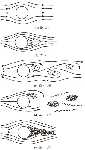
2.2.3 Kármán Vortex Street

Kármán vortex street is a repeating pattern of swirling vortices caused by vortex shedding,

which is responsible for the unsteady separation of flow of a fluid around bluff bodies. It is named

after Theodore von Kármán, who first systematically described it in 1912 as further development

of the prior result by Mallock and Bénard [52].

When a flow passes over a cylinder, Kármán vortex street will appear in certain conditions

related to the Reynolds number. WhenReis less than1, the upstream flow and downstream flow are symmetric, as shown in Figure 2.1(a). WhenRe∼5−40, steady vortices (Fopple vortex) are found attached to the trailing edge of the cylinder, as shown in Figure 2.1(b). WhenRereaches 40, an instability is observed in the form of an oscillation of the wake. The vortices start to peel

off from the rear of the cylinder regularly and periodically when Reis around 100, as shown in Figure 2.1(c). This is the Kármán vortex street after a cylinder. The flow remains laminar until

Reapproaches400, when turbulence starts to appear within the vortices, while the periodicity still remains. This structure is retained untilRereaches a dimension of104 ₋₁₀5_{, as shown in Figure}

(38)

(a) Re1

(b) Re∼10

(c) Re∼100

(d) Re∼104

(e)Re∼106

(39)

2.2.4 Dimensionless Quantities Used in This Study 2.2.4.1 Reynolds Number

Reynolds number is the ratio of inertial forces ρ ~U2_/D _{to the viscous force} _{µ ~}_{U /D}2_{, and it}

represents the level of disturbance in a flow. WhenReis small, the viscous force has a significant influence on the flow field, leading to attenuation of small disturbances, which makes the flow

become stable and laminar. Conversely, the inertial forces have a dominant role at a high Reynolds

number, which amplifies small disturbances. The flow has more possibility of becoming unsteady

and turbulent.

Reynolds number is defined as follows:

Re= ρU D

µ = U D

ν (2.29)

whereDis the characteristic linear dimension. In this case, it is the side length of the square cylinder or the diameter of the circular cylinder.

2.2.4.2 Strouhal Number

Strouhal number is a dimensionless number describing the oscillating flow mechanisms. It

represents the vortex shedding intensity of the flow. For large Strouhal numbers (St ∼1), viscos-ity dominates the fluid flow, resulting in a collective oscillating movement of the fluid. For low

Strouhal numbers (St <10−4_{), the steady state portion of the movement dominates the oscillation}

[46].

Strouhal number is defined as follows:

St = f D

U (2.30)

(40)

2.2.4.3 Drag Coefficient

Drag coefficient is a dimensionless quantity that is used to quantify the drag or resistance of an

object in a fluid environment. It is defined as follows:

Cd = 2Fd

ρU2_A (2.31)

(41)

CHAPTER 3 NUMERICAL SIMULATION

3.1 Method Introduction

In this chapter, the numerical simulations of five cylinders are described. Each simulation performs

calculations on a cylinder model, with the shape gradually changing from a square to a circle. The

detailed geometry of each cylinder is introduced in Chapter 3.1.1.

Simulations were performed in two dimensions for Reynolds numbers from 10 to 200 using

ANSYS FLUENT 18.2. In this chapter, a thorough discussion of the computational domains, grids,

and solvers used in this study are described.

3.1.1 Geometry Model Formation

Five cylinder models were formed using the software SOLIDWORKS 2018 and exported as

.IGS files, which were imported into the pre-process software of ANSYS FLUENT known as

ANSYS GAMBIT. The five cylinders are named C1 toC5 in sequence. C1 is a square cylinder

with a side length of0.375inch, i.e.r/D = 0. C2toC4 are three rounded-corner square cylinders

with the same side length and corner radii of 0.062, 0.092, and 0.125 inches, with r/D ratios of 0.167, 0.247, and 0.333, respectively. C5 is a circular cylinder with a diameter of 0.375 inch

(r/D= 0.5). The cross-sections are shown in Figure 3.1.

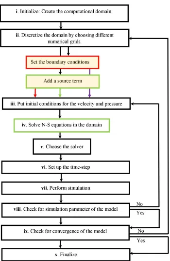
3.1.2 Main Process of Simulation

The flowchart of the main process of simulation is shown in Figure 3.2. After the generation

of cylinder geometry, there are ten steps to complete the simulation as follows:

(42)

Figure 3.1. Cross-Sections of CylindersC1toC5 (From Left to Right)

A computational domain needs to be set up first, with the cylinder geometry and walls. It

needs to be considered that the dimension of the domain should contain enough space to

clearly illustrate the flow structure but not too big to cause heavy computational burden.

2. Discretizing the domain by grids:

It is essential to choose the proper type and quantity of grids to discretize the domain, with

sufficient tests and modifications, as shown in Chapter 3.2.2 and Chapter 3.2.3.

3. Determining initial conditions:

The initial conditions together with the boundary conditions and source term is determined

in this step. In this study, all simulations were performed under atmospheric pressure and

25◦C, and the velocities were based on the Reynolds numbers needed.

4. Solving the N-S equation in the domain.

5. Choosing the CFD solver:

In this study, the Gauss-Siedel iterative method in conjunction with the Algebraic Multigrid

(AMG) was chosen as the solver; detailed discussion is provided in Chapter 3.1.3.

6. Setting up the time-step:

The time step was set to vary from0.01for steady flow to0.05for unsteady flow.

(43)

8. Checking for simulation parameter of the model:

If the parameter does not make physical sense after simulation, we need to go back to step 3

for modification.

9. Checking for convergence of the model:

If the simulation result shows divergence, there might be a problem with grid discretization

or choice of solver.

10. Finalizing:

Export all data to the post-processing software. The results are shown in Chapter 5.1.

3.1.3 CFD Solver and Numerical Method

The governing equations in Chapter 2.1 are a typical set of partial differential equations (PDEs).

To approximate those PDEs, it is necessary to choose an appropriate discretization method, e.g.,

finite difference method (FDM), finite volume method (FVM), and finite element method (FEM),

which are basically embedded in most commercial software. However, there are also other methods

such as spectral scheme, boundary element method (BEM), etc. After choosing the discretization

method, the discretization process is conducted with it. The discretization process is performed to

convert a set of PDEs into non-linear algebraic equations. For unsteady flows, an elliptic problem

is solved at each time step, while steady flows are solved using an equivalent iteration scheme.

Then, the problems turn out to be solutions of linear equation systems. The convergence criteria

are checked after completing all the calculations. The repetition of the loop depends on whether

the convergence is satisfied.

The commercial software ANSYS FLUENT 18.2 has been employed to simulate the present

problem using the control volume technique. A density-based (coupled) solver has been

imple-mented for pressure-velocity coupling, while the algebraic equations are solved using SIMPLE

scheme [32]. The discretization of convective terms is performed by FVM, specifically, by the

(44)

(45)

AMG method can significantly reduce the number of iterations (and thus, CPU time) required to

obtain a converged solution, especially when the model contains a large number of control

vol-umes. The time step varies from0.01for steady flow to0.05for unsteady flow. The convergence criteria for the inner (time step) iterations are set as10−8_{for the discretized continuity, momentum}

equations, and the discretized energy equation.

3.2 Parameter Settings

After determining the adequate numerical method for calculation, it is essential to set up the

bound-ary conditions, the computational domain, and other parameters before starting the simulation. In

addition, it is important to choose the appropriate mesh quantity and grid type through mesh

inde-pendence study and grid type study.

3.2.1 Boundary Conditions

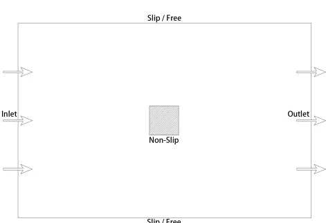
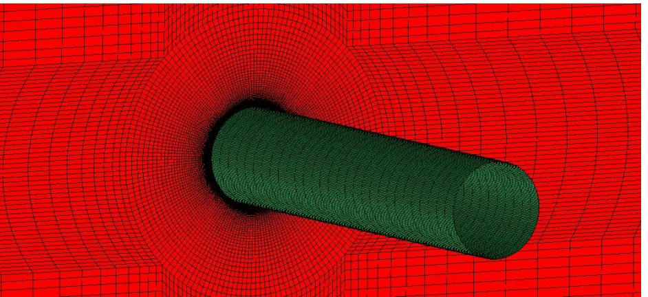
The boundary for the bluff body used in this simulation is shown in Figure 3.3. It should be

noted that the scale in this figure is not actual. The cylinder is enlarged three times so that it can

be seen clearly. In this rectangular box, the left boundary was set as the flow inlet and the right

boundary was set as the pressure outlet. Also, all four wall boundaries were set as the slip wall to

model an undisturbed flow channel. The cylinder boundary was set as a non-slip wall to make sure

that there was no relative movement between the boundary and the fluid layer.

The cylinders were placed in the geometric center of the computational domain. The size of

the computational domain is discussed in the next section. Considering that the fluid is air under

atmospheric pressure and25◦C, all the simulations were conducted at a Prandtl number (P r) equal to0.73.

3.2.2 Computational Domain and Mesh Independence

To evaluate the domain sensitivity, three computational domains were tested, namely G1, G2,

and G3. The domain sizes L×H of 25D ×20D, 30D×20D, and50D×20D were studied.

(46)

(47)

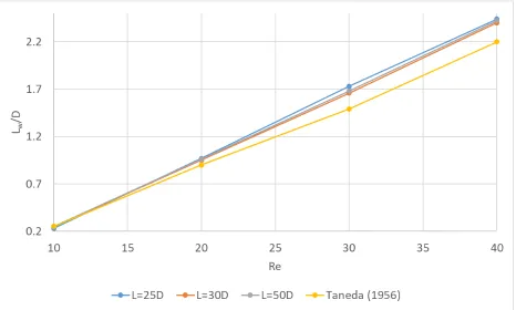
107,240(nodes: 106,484, Figure A.5), and201,040(nodes:200,364, Figure A.6). TakingC5as an example, the comparison results are shown in Table 3.1 and Figure 3.4. Lw is defined as the length of Föppl vortices andLw/D is the scaled reattachment length behind the cylinder.

G1 (L= 25D) G2(L= 30D) G1(L= 50D) Taneda (1956) [48]

n∗ 101280 107240 201040 –

Re Cd Lw/D Cd Lw/D Cd Lw/D Lw/D 10 3.0478 0.23 3.0291 0.25 3.0213 0.25 0.25 20 2.1697 0.97 2.1585 0.95 2.1528 0.96 0.90 30 1.8134 1.73 1.8045 1.66 1.7997 1.68 1.49 40 1.6090 2.44 1.6014 2.40 1.5970 2.42 2.20

∗: Mesh Numbers

Table 3.1.Computational Domain Study

Figure 3.4.Computational Domain Comparison

It is shown in Table 3.1 and Figure 3.4 that G2 has the most accuracy of scaled reattachment

(48)

also suggested the size of the computational domain to be around30Din length. Therefore,G2 is

chosen for the computational domain size and grid quantity for further study.

To ensure the mesh density does not affect the simulation result, mesh independence study was

also carried out, with tested mesh size ofξmax = 100,150,200. ξmaxis the maximum grid quantity downstream of the cylinder. It is shown that ifξmaxis greater than 150, the flow parameters (drag coefficient) does not change with the grid size. As the result,ξmax = 150is used for further study.

3.2.3 Grid Type

The computational domain is represented by numerical grids, in which the variables can be

calculated. There are different types of numerical grids for the flow solver, and they can be roughly

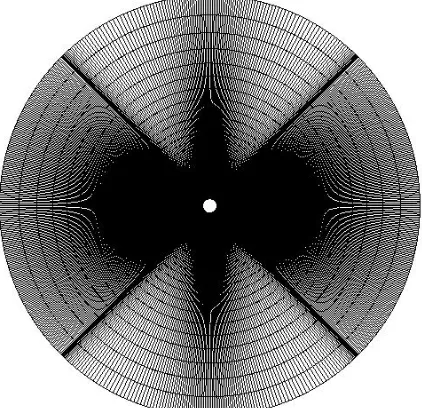
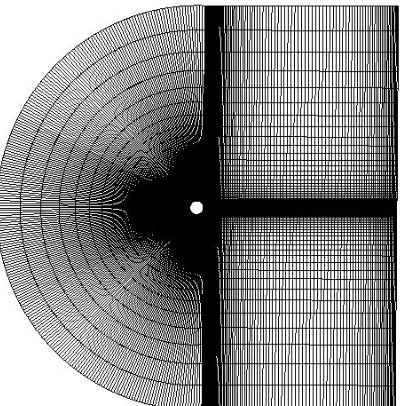
classified as structured and unstructured grids [11] [45]. Structured grids include three basic types:

H-, O-, and C-types. The names are derived from the shapes of the grid lines. These three types

of grids are shown in Figures A.1, A.2, and A.3, respectively. In the simulations, all three types of

grids are compared. Also, by takingC5as an example, the comparison results are shown in Table 3.2 and Figure 3.5.

Re H-Grid O-Grid C-Grid Taneda (1956) [48]

Cd Lw/D Cd Lw/D Cd Lw/D Lw/D 10 3.0291 0.25 2.9146 0.25 2.7337 0.26 0.25 20 2.1585 0.95 2.1062 0.98 2.1583 0.72 0.90 30 1.8045 1.66 1.7660 1.67 1.7826 1.36 1.49 40 1.6014 2.40 1.5698 2.40 1.5812 2.01 2.20

Table 3.2.Grid Type Study

It is shown in Table 3.2 and Figure 3.5 that the H-type grid has the most accuracy of scaled

reattachment length compared with Taneda’s experiment (1956). Therefore, the H-type grid is

chosen as the grid type for further study.

By using all these parameters that were determined, five cylinders were simulated, and the final

(49)

(50)

CHAPTER 4 WIND TUNNEL EXPERIMENT

4.1 Experimental Facilities

The experiments were performed in an Engineering Laboratory Design (ELD) Model 404 wind

tunnel located in Kingsbury Hall at the University of New Hampshire. The test-section dimensions

are 18 inch x 18 inch cross-section and 36 inch in length with a maximum speed of 150 mph.

measured using a Pitot-static tube connected to a differential pressure transducer.

The wind tunnel is an Eiffel type tunnel. Air is drawn into the radiused inlet through a

honey-comb and screen pack and is accelerated through the contraction into the test section. The system

air regains static pressure when passing through the diffuser and is discharged to the atmosphere.

The test section is fabricated using a 3/4”thickness acrylic plexiglass on the top, sides, and bottom, with interior dimensions of36”in length,18” in width, and18”in height. The side wall

on the operating side of the test section is fitted with a7”high by 8”wide access opening at the

center, while the other side is a hole of 0.5” with LabVIEW drag force sensor set. A Pitot tube is placed along the center line of the test section, extending 5” cm from the ceiling of the test

section. It is connected to a water column pressure gauge, from which the pressure difference can

be recorded according to the water head, and then the wind speed can be derived.

The fan assembly is capable of providing a total of 9 levels of wind speed, with the maximum

(level 9) being65m/s and the minimum (level 1) being2m/s. During the experiment, only level 2

(51)

(a) Inlet (b) Contraction

(c) Test Section (d) Fan and Diffuser

Figure 4.1.Sketch Map of Wind Tunnel for Experiment

(52)

The wind tunnel sketch map (in parts) is shown in 4.1, and the assembly drawing is shown in

Figure 4.2.

4.2 Operation Steps

The main processes of the experiment are as follows:

1. Recording the temperature in the laboratory:

The room temperature was recorded using a mercury thermometer for calculating the air and

water density.

2. Zeroing the Pitot tube and the drag force sensor with a cylinder plugged in:

Every time when switching to a new cylinder, the clamp needed to be re-tightened, which

resulted in minor displacement in the sensor. It was reflected in the drag force deviation on

the screen. Thus, it was necessary to set the drag force to zero once a new cylinder was

replaced into the tunnel.

3. Recording the water head difference from the water column pressure gauge:

The water head difference was recorded so that it was possible to calculate the difference

between the total pressure and static pressure in the flow, and subsequently the wind speed.

4. Recording the drag force data from the sensor:

The drag force was recorded so that the drag coefficient could be derived together with the

wind speed.

5. Switching the wind speed level and repeating Steps 3 - 4:

Every cylinder was tested under wind speeds of level 2 to level 8.

6. Replacing the cylinder and repeating Steps 2 - 5:

A total of five cylinders were tested. The cylinder geometry is the same as that in the

(53)

In all the processes, the drag force of every cylinder under different Reynolds numbers were

collected successfully. The original data is shown in Table B.1.

4.3 Data Processing

In this section, the formulas for deriving the drag coefficient from the original data are introduced

in steps.

4.3.1 Dynamic Pressure

According to the knowledge of the Pitot tube, the higher water column represents the total

pressure while the lower water column represents the static pressure. The water head difference

represents the pressure difference, which is the dynamic pressure related to wind speed.

The dynamic pressurepdcan be derived as follows:

pd =ρwg∆h (4.1)

whereρw is the density of water. It depends on the recorded room temperature, which can be looked up in Table B.3 [14].

It should be noted that the data of∆hwas recorded in units of inches. Equation 4.1 is modified to convert∆hinto international system of units:

pd= 0.0254ρwg∆h (4.2)

4.3.2 Wind Speed

According to Bernoulli’s principle, the relationship between the dynamic pressure and wind

speed is

pd= 1 2ρaU

2

(4.3)

(54)

By substituting Equation 4.2 and some transposition, we get

U = s

0.0508ρwg∆h

ρa

(4.4)

4.3.3 Reynolds Number

According to Chapter 2.2.4.1, the Reynolds number can be derived as follows:

Re= ρaU D

µ (4.5)

The air dynamic viscosityµdepends on the recorded room temperature, which can be looked up in Table B.4 [14].

By substituting Equation 4.4 and modifying the unit of side lengthD(from inches to meters), we get

Re= 0.0254D

µ

p

0.0508ρwρag∆h (4.6)

By substituting all constants ofD= 0.375inches andg = 9.8m2/s, we get

Re= 0.00672

√

ρwρa∆h

µ (4.7)

4.3.4 Drag Coefficient

According to Chapter 2.2.4.3, the drag coefficient can be derived as follows:

Cd= 2Fd

ρaU2A

(4.8)

where Ais the reference surface area, which in this study is the windward projection area of the cylinder, i.e.,L0×D. Excluding the parts held by the sensor clamp, the length in the flow field

L0 is7inches.

(55)

Cd=

23245.7Fd

ρwg∆h

(56)

CHAPTER 5 RESULT ANALYSIS

5.1 Numerical Simulation on Low Reynolds Number

5.1.1 Simulation validity Examination

Based on the discussion of Chapter 3, the mesh type of H-grid and computational domain of

L= 30DandH = 20Dwere chosen to simulate the flow. Under the conditions mentioned above, the flow around the circular cylinder was first tested to verify the formation of Föppl’s vortices

and Kármán vortex street discussed by Taneda [48] [49] and Rushko [42]. The simulated flow

structures are shown in Figure A.24 (Re = 10 −40) and Figure A.25 (Re = 60− 200). The streamlines are shown in Figure A.26 (Re= 10−40) and Figure A.27 (Re= 60−200).

For the simulation results mentioned above, it is clear that whenRe₆40, the shedding vortex does not appear and the downstream flow is considered to be steady. Meanwhile, a pair of Föppl’s

vortices is observed behind the cylinder, which matches the studies of Taneda and Rushko.

Under the condition of Re _> 60, an unsteady oscillation accompanied with periodic vortex shedding is observed behind the cylinder. The oscillation range increases with increase in the

Reynolds number.

The data of the drag coefficient are exhibited in Figure 5.1 and compared with the experimental

and simulation results from Tritton (1959) [50], Dennis (1970) [9], Park (1998) [30], Clift (2005)

[6], and Gabitto (2008) [13]. Owing to the similarity between the results of the present study and

(57)

Figure 5.1.Simulation Validation Examination – Drag Coefficient Comparison

Re C1 (r/D=0) C2 (r/D=0.167) C3 (r/D=0.247) C4 (r/D=0.333) C5 (r/D=0.5)

10 0.52 0.51 0.5 0.42 0.25

20 1.3 1.22 1.2 1.1 0.95

30 2 1.8 1.75 1.7 1.66

40 2.6 2.4 2.3 2.25 2.4

(58)

5.1.2 Scaled Reattachment Length, Strouhal Number, and Drag Coefficient under Effect of Corner Radius

Through numerical simulation, cylinders with different Reynolds numbers and of various

cor-ner radii were tested with the abundant data acquired. To illustrate the flow structure evaluation

under the effect of corner radius, three main parameters were taken for comparison, including the

scaled reattachment length (Lw/D), Strouhal number (St), and drag coefficient (Cd).

5.1.2.1 Scaled Reattachment Length

The scaled reattachment length is defined as the length of Föppl’s vortices divided by the

cylin-der’s side length. It is only valid in the steady condition, i.e. Re₆40. The data is shown in Table 5.1 and Figures 5.2 and 5.3.

Figure 5.2.Scaled Reattachment Length VS Reynolds Number

From Figure 5.2, we can see that the scaled reattachment length has a positive correlation with

(59)

Figure 5.3.Scaled Reattachment Length VS Corner Radius Ratio

findings of the previous study that Föppl’s vortices stretch when the Reynolds number increases.

In general, the greater the corner radius ratio of a cylinder, the shorter its scaled reattachment

length. However, in the figure, it is seen that the only exception is C5, a circular cylinder, at a Reynolds number of 40. Its scaled reattachment length is greater than that of the three cylinders

with lower corner radius ratios. Figure 5.3 is drawn to show this more clearly, and from this figure,

we can see that the only case in which Lw/D increases is when r/D = 0.5 and Re = 40. It is probably due to the precocious separation of the boundary layer on the circular cylinder. The

separation range ofC4is about90◦in the leeward section, whileC5is around120◦, which can be noted when comparing Figures A.22.(d) and A.26.(d).

Another property shown in Figure 5.3 worth noticing is that the scaled reattachment length

has the least sensitivity to Reynolds number at r/D ≈ 0.25, which means that Föppl’s vortices range is the steadiest at this corner radius ratio, with the smallest stretching. It may be helpful for

(60)

flow with various Reynolds numbers, i.e., when the point should not fall into or leave the Föppl’s

vortices when the Reynolds number changes.

5.1.2.2 Strouhal Number

The Strouhal number, as described in Chapter 2.2.4.2, represents the vortex shedding intensity

of the flow. Under the same conditions of flow velocity and object size, the higher Strouhal number

indicates a higher frequency of vortex shedding. In contrast to the scaled reattachment length,

Strouhal number is only valid in the unsteady range, i.e. Re_> 60, from which the Kármán vortex street starts to form. The data is shown in Table 5.2 and Figures 5.4, 5.5.

Figure 5.4.Strouhal Number VS Reynolds Number

As shown in Figure 5.4, unlike the scaled reattachment length, the Strouhal number does not

have a linear correlation with the corner radius ratio. Statistically, C1 and C5 have the lowest Strouhal numbers, which means that the vortex shedding frequency of the square and circular

(61)

rounded-Re C1 (r/D=0) C2 (r/D=0.167) C3 (r/D=0.247) C4 (r/D=0.333) C5 (r/D=0.5)

60 0.104 0.105 0.118 0.123 0.125

100 0.143 0.185 0.195 0.192 0.16

150 0.157 0.211 0.203 0.216 0.188

200 0.188 0.235 0.224 0.244 0.193

Table 5.2.Strouhal Number Comparison