University of Pennsylvania
ScholarlyCommons
Publicly Accessible Penn Dissertations
1-1-2012
Development of High Angular Resolution
Diffusion Imaging Analysis Paradigms for the
Investigation of Neuropathology
Luke Bloy
University of Pennsylvania, [email protected]
Follow this and additional works at:
http://repository.upenn.edu/edissertations
Part of the
Biomedical Commons
, and the
Radiology Commons
This paper is posted at ScholarlyCommons.http://repository.upenn.edu/edissertations/493
For more information, please [email protected].
Recommended Citation
Bloy, Luke, "Development of High Angular Resolution Diffusion Imaging Analysis Paradigms for the Investigation of Neuropathology" (2012).Publicly Accessible Penn Dissertations. 493.
Development of High Angular Resolution Diffusion Imaging Analysis
Paradigms for the Investigation of Neuropathology
Abstract
Diffusion weighted magnetic resonance imaging (DW-MRI), provides unique insight into the microstructure of neural white matter tissue, allowing researchers to more fully investigate white matter disorders. The abundance of clinical research projects incorporating DW-MRI into their acquisition protocols speaks to the value this information lends to the study of neurological disease. However, the most widespread DW-MRI technique, diffusion tensor imaging (DTI), possesses serious limitations which restrict its utility in regions of complex white matter. Fueled by advances in DW-MRI acquisition protocols and technologies, a group of exciting new DW-MRI models, developed to address these concerns, are now becoming available to clinical researchers.
The emergence of these new imaging techniques, categorized as high angular resolution diffusion imaging (HARDI), has generated the need for sophisticated computational neuroanatomic techniques able to account for the high dimensionality and structure of HARDI data. The goal of this thesis is the development of such techniques utilizing prominent HARDI data models. Specifically, methodologies for spatial normalization, population atlas building and structural connectivity have been developed and validated. These methods form the core of a comprehensive analysis paradigm allowing the investigation of local white matter
microarcitecture, as well as, systemic properties of neuronal connectivity. The application of this framework to the study of schizophrenia and the autism spectrum disorders demonstrate its sensitivity sublte differences in white matter organization, as well as, its applicability to large population DW-MRI studies.
Degree Type
Dissertation
Degree Name
Doctor of Philosophy (PhD)
Graduate Group
Bioengineering
First Advisor
Ragini Verma
Keywords
Diffusion MRI, FOD, HARDI
Subject Categories
DEVELOPMENT OF HIGH ANGULAR RESOLUTION DIFFUSION IMAGING ANALYSIS PARADIGMS FOR THE INVESTIGATION OF NEUROPATHOLOGY
Luke Bloy
A DISSERTATION
in
Bioengineering
Presented to the Faculties of the University of Pennsylvania
in
Partial Fulfillment of the Requirements for the
Degree of Doctor of Philosophy
2012
Supervisor of Dissertation
Ragini Verma, Associate Professor, Radiology, UPenn
Graduate Group Chairperson
Beth Winkelstein, Professor, Bioengineering, UPenn
Dissertation Committee
Timothy P. L. Roberts, Profesor, Radiology, UPenn
Andrew Tsourkas, Associate Professor, Bioengineering, UPenn Ragini Verma, Associate Professor, Radiology, UPenn
Felix Wehrli, Professor, Radiology, UPenn
This work is dedicated to my family:
ACKNOWLEDGEMENT
This thesis, and more importantly the research that it describes, are the culmination of more than four years of work. It would not have been possible without the support and effort of many people who have contributed to it as well as to my development as a scientist, to whom I am deeply indebted.
Firstly, I would like to thank my mentor, Dr. Ragini Verma. Ragini has always been incredibly supportive and encouraging. Our endless discussions were crucial to development of the ideas and problems central to this research, and provided valuable insight and training in the many skills required by the modern research environment.
In many ways research is a collaborative effort and I have been lucky enough to work in a lab full of excellent researchers, who have made coming to work each day both interesting and fun. For this I thank Dr. Christos Davatzikos and Dr. Verma for assembling this group of people and creating an engaging and focused atmosphere in which to work. I am particularly thankful to Madhura Ingalhalikar, Drew Parker, Alex Smith, Yasser Ghanbari and Kayhan Batmanghelich, who were a sounding board for all of my ideas, no matter how absurd, and were central to the identification and development of the good ones. I would also like to thank Mark Bergman, Evi Parmpi and Amanda Shacklett for all of their help in navigating the many facets of being a graduate student.
ABSTRACT
DEVELOPMENT OF HIGH ANGULAR RESOLUTION DIFFUSION IMAGING ANALYSIS PARADIGMS FOR THE INVESTIGATION OF NEUROPATHOLOGY
Luke Bloy
Ragini Verma
Diffusion weighted magnetic resonance imaging (DW-MRI), provides unique insight into the microstructure of neural white matter tissue, allowing researchers to more fully investigate white matter disorders. The abundance of clinical research projects incorporating DW-MRI into their acquisition protocols speaks to the value this information lends to the study of neurological disease. However, the most widespread DW-MRI technique, diffusion tensor imaging (DTI), possesses serious limitations which restrict its utility in regions of complex white matter. Fueled by advances in DW-MRI acquisition protocols and technologies, a group of exciting new DW-MRI models, developed to address these concerns, are now becoming available to clinical researchers.
TABLE OF CONTENTS
ACKNOWLEDGEMENT . . . iii
ABSTRACT . . . iv
LIST OF TABLES . . . viii
LIST OF ILLUSTRATIONS . . . ix
CHAPTER 1 : Introduction . . . 1
CHAPTER 2 : Diffusion Weighted MRI in Neuroimaging . . . 8
2.1 Principles of DW-MRI . . . 8
2.2 The Diffusion Tensor Model . . . 10
2.3 Beyond the DT Model . . . 13
2.4 Applications of DW-MRI in Clinical Populations . . . 17
2.5 The Anatomy of a Population Study . . . 20
CHAPTER 3 : HARDI Spatial Normalization . . . 23
3.1 Introduction. . . 23
3.2 FOD-based Non-Linear Spatial Normalization . . . 24
3.3 Validation: Simulated Experiments . . . 30
3.4 Validation: In-vivo Experiments . . . 32
3.5 Conclusions . . . 37
CHAPTER 4 : White Matter Parcellation . . . 39
4.1 Introduction. . . 39
4.2 White Matter Parcellation . . . 42
4.4 Development of a Adolescent WM Atlas . . . 47
4.5 Conclusions . . . 52
CHAPTER 5 : Structural Connectivity. . . 55
5.1 Introduction. . . 55
5.2 An Integrated Structural Connectivity Framework . . . 57
5.3 Validation: In-vivo Human Datasets . . . 64
5.4 Discussion . . . 71
CHAPTER 6 : Applications . . . 76
6.1 Introduction. . . 76
6.2 Analysis Framework . . . 77
6.3 Schizophrenia: Results and Discussion . . . 81
6.4 Autism: Results and Discussion . . . 87
6.5 Conclusion . . . 92
CHAPTER 7 : Conclusion . . . 93
CHAPTER A : Datasets and Common Preprocessing . . . 98
A.1 Imaging Datasets . . . 98
A.2 Processing Pipeline . . . 100
Appendix B : The Real Spherical Harmonics . . . 102
B.1 Mathematical Definition . . . 102
B.2 Rotations in the RSH basis . . . 103
B.3 Spectral Powers of the RSH . . . 104
B.4 Established Metrics. . . 105
Appendix C : Publications . . . 107
LIST OF TABLES
TABLE 6.1 : Applications: Structural Connectivity Differences in SCZ . . . 85
LIST OF ILLUSTRATIONS
FIGURE 1.1 : Gross Dissections of the Cerebral Hemisphere . . . 2
FIGURE 1.2 : Robustness of the FOD . . . 5
FIGURE 2.1 : Stejskal and Tanner PGSE sequence . . . 9
FIGURE 2.2 : Simulation of 90◦fiber crossing geometry . . . 12
FIGURE 3.1 : Registration: FOD registration pipeline . . . 26
FIGURE 3.2 : Registration: FOD Reorientation . . . 27
FIGURE 3.3 : Registration: Registration Accuracy in Simulated data . . . 31
FIGURE 3.4 : Registration: Effect of FODs order on Registration . . . 32
FIGURE 3.5 : Registration: DTI and FOD Population Variance Images . . . 35
FIGURE 3.6 : Registration: T-Tests between DTI and FOD registration residuals 36 FIGURE 3.7 : Registration: Ability to register cortical WM . . . 37
FIGURE 4.1 : WM Parcellation: Simulated Fiber Cross . . . 47
FIGURE 4.2 : WM Parcellation: Clustering Parameters . . . 49
FIGURE 4.3 : WM Parcellation: Clustering Symmetry. . . 50
FIGURE 4.4 : WM Parcellation: High Resolution Atlas . . . 50
FIGURE 4.5 : WM Parcellation: Comparison with Anatomical Atlas. . . 51
FIGURE 5.1 : Structural Connectivity Framework Diagram . . . 58
FIGURE 5.2 : Structural Connectivity Transition probability . . . 59
FIGURE 5.3 : Structural Connectivity: Test/Retest . . . 66
FIGURE 5.4 : Structural Connectivity: Inter/Intra Subject Sensitivity . . . 67
FIGURE 5.5 : Structural Connectivity: Connectivity Matrics . . . 68
FIGURE 5.6 : Structural Connectivity: Nodal Connection Distribution . . . 69
FIGURE 5.7 : Structural Connectivity: Connections of the Corpus Callosum . . 69
FIGURE 5.9 : Structural Connectivity: Comparison to WholeBrain TDI. . . 72
FIGURE 6.1 : Applications: ASD and SCZ Atlases . . . 79
FIGURE 6.2 : Applications: Voxel Statistics in Schizophrenia (Males) . . . 82
FIGURE 6.3 : Applications: Voxel Statistics in Schizophrenia (Females) . . . 84
FIGURE 6.4 : Applications: Regional Statistics in Schizophrenia . . . 84
FIGURE 6.5 : Applications: Connectivity Statistics in Schizophrenia . . . 86
FIGURE 6.6 : Applications: Voxel Statistics in ASD . . . 89
CHAPTER 1 : Introduction
The human brain consists of approximately 100 billion neurons, organized into a vastly complex network of interconnections. This network, consisting of both local neural circuits and long distance fiber pathways, is thought to provide the anatomical substrate allowing for the distributed interactions between brain regions [70,128,157]. While neural anatomy has been extensively studied using cerebral dissection [66, 144], relatively little is known about this complex set of connections which mediate brain function and give rise to the richness of human behavior and experience. Chemical tracing, where markers are locally injected into the cortex and their subsequent distribution is observed, has facilitated the probing of this network yielding connectivity information in many animal models [110,145]. However, the invasiveness of this technique precludes its use in human subjects particularly, within a clinical setting.
More recently, diffusion weighted magnetic resonance imaging (DW-MRI) has emerged as the prominent noninvasive methodology able to quantitatively probe neuronal white mat-ter (WM), enabling the in-vivo investigation of tissue microstructure and organization. By describing the average molecular diffusion of water molecules, DW-MRI probes tissue structure at biological scales typically unavailable to noninvasive imaging techniques. The fact that water molecules in highly organized fibrous tissues, such as neuronal WM, diffuse preferentially along fibers, allows DW-MRI to obtain information related to the local tissue architecture. This knowledge of the local WM organization can also be extrapolated to infer global patterns of neuronal connectivity, previously available only via dissection, as in Figure1.1, or chemical tracing techniques. The ability to investigate both local architecture and global structural connectivity, in-vivo, has garnered DW-MRI an important place in many clinical studies focused on evaluating WM tissue structure, fidelity and development.
Figure 1.1: Illustrations by Friedrich Arnold [10] of gross dissections of the cerebral hemi-sphere. From [145, Schmahmann2007a].
complexity of the mathematical models used to represent the diffusion signal has continually increased. Initially a single scalar, the apparent diffusion coefficient (ADC) [23], was used to measure the degree of diffusion at each voxel. Subsequent improvements in MR hardware and image acquisition have led to improved signal to noise (SNR), enabling a more formal treatment of in-vivo diffusion, the diffusion tensor (DT) model [17], to be developed.
The use of a Gaussian distribution of molecular displacements allows diffusion tensor imag-ing (DTI) to model molecular diffusion in three dimensions enablimag-ing researchers to quantita-tively investigate the amount of diffusion per voxel (the ADC), its anisotropy (the acuteness of its directionality), as well as its spatial orientation. The more robust information avail-able from the DT model has proved to be very useful in the study of both normal and pathological brains, as discussed in section 2.4. DTI is now routinely included in research protocols studying a range of pathologies, such as multiple sclerosis [35,75], schizophrenia [96], autism [26,87], as well as normal development [64].
without limitations. Most importantly, its dependence on a single Gaussian distribution limits its ability to model architectures with multiple fiber orientations. Voxels with a more complex microarchitecture, such as fiber crossings or fanning configurations, are thus poorly characterized. This represents a serious limitation, as it is currently thought that between one and two thirds of the WM voxels [21], at the current clinical resolutions of 1-3 mm isotropic, show evidence of complex fiber organization [133, 174]. The recognition of this limitation has led to the development of a group of more complex diffusion models that are better able to describe the complexities of these tissue architectures.
Diffusion spectrum imaging (DSI) exploits the Fourier relationship [172,183,181] between the DW-MRI signals and the underlying diffusion process to compute a three dimensional probability distribution function (PDF), at every imaging voxel, describing the local dif-fusion process. In an attempt to reduce the high data acquisition requirements of DSI, other models have been introduced that have lower acquisition requirements. The most prominent, the orientation distribution function (ODF) [2,47,170,173] and the fiber orien-tation distribution (FOD) [8,168], require a single shell DW-MRI acquisition and are often referred to as high angular resolution diffusion imaging (HARDI) [173] diffusion models.
The focus of this thesis is the development of such an analysis framework. Two types of analysis are enabled by the methods developed here. First, local features derived directly from the diffusion models can be used to investigate regional differences in WM architecture. This necessitates the establishment of the spatial correspondence between the WM anatomy of each subject, which is accomplished through the developed HARDI-based spatial nor-malization process. Homogeneous WM regions of interest (ROIs) can then be defined by parcellating the WM volume based on its local architecture, thereby enabling the generation of population specific atlases and facilitating regional statistics. The second type of analysis, is achieved through the development of a structural connectivity algorithm. Registration is again used to establish spatial correspondence between subjects, in this case between the gray matter (GM) nodal regions. This correspondence enables the direct statistical analysis of the connection strengths, in addition to the analysis of the global topological features of these networks. Combined, these tools form the core of a HARDI neuroimaging toolkit, from which more complex statistical analysis methods can be developed in the future.
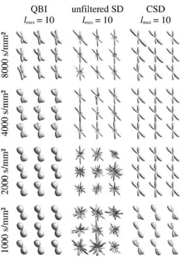
Figure 1.2: Orientation distribution function (QBI) and FODs computed with spherical deconvolution and constrained spherical deconvolution, are shown for a range of b-values. The CSD produces more robust profiles then either the QBI or the SD. Adapted from [168, Tournier 2008].
Organization and Contributions of this Thesis
mathemat-ics of the RSH basis functions, that form the core of our analysis methods, are discussed in AppendixB. In combination, these present the requisite background information required to place the remainder of this work in context. The main contributions of the thesis are then presented as independent chapters.
The spatial normalization method, presented in Chapter 3, utilizes the RSH coefficients of the FOD data model to inform a diffeomorphic Demons registration framework used to align each subject’s anatomy with that of a template subject. The method is a two phase framework, using an orientation invariant approach in the initial phase followed by an orientation sensitive secondary phase. Simulation studies show that this overall approach is able to maintain the registration accuracy achieved from the more intensive orientation sensitive method, in reduced computational time. The proposed approach is also compared with state of the art DTI-based registration techniques, illustrating the ability of the HARDI based approach to better align the WM anatomy, as indicated by lower population variances, lower residuals and improved overlap of the population’s WM volumes.
Chapter4describes a data-driven WM parcellation algorithm which utilizes local variations in an FOD image to delineate regions of homogeneous tissue architecture. This approach allows the generation of population specific atlases at various levels of granularity, enabling researchers to tailor the process to their specific application. The use of a local similarity measure and an iterative process, focused on minimizing regional variance, yields ROIs that are more homogeneous then those typically available from anatomically defined atlases.
It should be noted that while the above methods were all developed and validated using the FOD diffusion model, they can be seamlessly applied to any spherical diffusion model possessing a representation in the RSH basis. This ability provides a simple means for evaluating the utility of the alternate diffusion models within the context of a group study, while controlling for the analysis methods being used.
Finally, the utility of these methodologies to elucidate group differences is demonstrated through the investigation of two disorders, schizophrenia and autism, thought to possess a degree of aberrant connectivity. These studies illustrated the ability of the proposed methods to localize differences in both the WM microstructure and in the patterns of structural connectivity. While these preliminary findings are intriguing, additional studies with larger numbers of subjects are needed to replicated them. None the less, these studies serve as validation that the proposed methods are able to capture group differences and provide a solid basis from which additional analysis may be performed.
Software Contributions
CHAPTER 2 : Diffusion Weighted MRI in Neuroimaging
The focus of this thesis is the development of an analysis framework enabling the use of HARDI diffusion models within research studies of human WM and neuropathology. It is important to recognize that since DW-MRI became a viable in-vivo imaging modality in the early 1990s, the mathematical tools being used to investigate and model diffusion in the brain have undergone continuous development. The purpose of this chapter is to present this development with a particular focus on those models that are applicable to the framework developed in this thesis. Additionally, we present some of the insights that have been garnered using DTI within population studies, suggesting areas where the more complex HARDI modeling may be particularly beneficial.
2.1. Principles of DW-MRI
All particles, at temperatures above absolute zero, undergo random Brownian motion. Within populations or ensembles of particles, this random motion results in a diffusion process, where the population of particles gradually spreads. When concentration gradients exist this process explains the net movement of particles from regions of higher concen-tration to those of lower concenconcen-trations, although diffusion also occurs in the absence of a concentration gradient.
Figure 2.1: The Stejskal and Tanner pulsed gradient spin echo sequence. Adopted from [185, Westin2002]
directly related to the diffusion coefficient:
x2= 6Dτd
DW-MRI’s sensitivity to the diffusion process is due to the introduction, by Stejskal and Tanner [158], of a series of diffusion encoding pulse sequences prior to either a spectroscopic readout or an imaging pulse sequence. The most basic pulse sequence demonstrating this pre-encoding block, is the pulsed gradient spin echo (PGSE) sequence (seen in Figure2.1). The diffusion sensitivity is due to a pair of balanced linear gradients separated by a 180◦ pulse. These gradient pulses, separated by a time ∆, are applied along the directionuwith a strengthgfor a duration ofδ. The first gradient imparts each spin with a phase proportional to its location along the encoding direction. The 180◦ pulse inverts the spins allowing the second gradient, balanced in respect to time and magnitude, to refocus the spins. Those spins that do not experience any displacement along u, during the time separating the two gradient lobes, are completely refocused. However, those that have diffused along
u experience a slightly different field strength during the second gradient lobe than was experienced during the first resulting in an incomplete rephasing and a subsequent signal loss.
subsequent signal can be expressed by the common form of the Stejskal-Tanner equation:
S(u) =S0e−bD (2.1)
whereS(u) is the measured signal resulting from a gradient direction ofu,S0 is the signal in the absence of diffusion sensitive gradients (often referred to as a b0 image in DW-MRI).
Dis the diffusion coefficient or when used to describe the average response from a DW-MRI voxel, the apparent diffusion coefficient (ADC). The ’b-value’ [23],
b=γ2δ2
∆−δ
3
g2
is related to the gradient strength (g), the gyromagnetic ratio of water protons (γ) as well as the pulse duration (δ) and separation (∆). Typical DW-MRI acquisitions utilize ∆s on the order of 30-60 ms, meaning that DW-MRI is probing the tissue microstructure on length scales in the 23–32 µm range (assuming a D = 3x10⁻³mm/s), a scale much smaller then those available from other in-vivo imaging modalities.
It is important to note that each diffusion weighted image (DWI) is sensitive to a single diffusion direction, however, diffusion is a three dimensional process and water displacements may not be uniform in all directions [122]. This anisotropic diffusion may be due to the local tissue organization, such as membranes or other obstacles impeding diffusion in certain directions. The desire to account for this phenomenon has led to the development of a diffusion model capable of capturing the true anisotropic nature of the water diffusion in biological tissue, the DT model [17].
2.2. The Diffusion Tensor Model
within each imaging voxel as full three dimensional Gaussian process of the form:
P(x, τ) = 1
4πτ3|D|e
−1
4τx
tDx
(2.2)
where the probability of a displacement,x, occurring in a timeτis controlled by a symmetric 3x3 covariance matrix describing the Brownian motion of water molecules at each imaging voxel, the diffusion tensor (D). Using this form, the solution to the Stejskal-Tanner equation is:
S(u) =S0e−bu
tDu
(2.3)
The symmetric nature of the DT means that it posseses six unknown elements that must be estimated from the DWIs, requiring a minimum of six DWIs be acquired using non-colinear gradient directions, in addition to a single b0 image. Estimating the DT from these measurements has been extensively studied, with proposals ranging from traditional linear least squares approaches, to more sophisticated methods that account for the strict positivity of the diffusion process [11,54].
The largest benefit of the DT model is its ability to characterize the local diffusion pro-cess using measures beyond the ADC, which can be computed as 1/3 of the trace of the DT. An eigensystem analysis can be used to diagonalize the DT, identifying the principal diffusion directions (the eigenvectors), as well as, the diffusivity in those directions (the eigenvalues,λs). This yields information concerning both the shape and orientation of the diffusion process. Additionally, many scalars have been introduced to quantify the amount of anisotropic diffusion that is present in each voxel. For instance, the linear anisotropy (CL), planar anisotropy (CP), and spherical anisotropy (CS), have been proposed [185] to measure different types of anisotropy in each voxel. However, the most widely accepted measure remains the fractional anisotropy (FA) [19]. The FA measures the severity of the anisotropy of the DT by:
F A=
s
3 2
(λ1−λ¯)2+ (λ2−¯λ)2+ (λ3−¯λ)2
DT
ADC
ODF
Fiber Directions
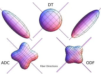
Figure 2.2: A simulated example of a simple crossing geometry where two fiber pathways intersect at 90◦. As can be seen the DT model is able to identify the fiber plane but is unable to distinguish the individual peaks representing each fiber population whereas the HARDI models, ODF and ADC, are better able to capture the complex structure. Only the peaks of the ODF align with the simulated fiber directions.
whereλ1,λ2 and λ3 are the eigenvalues of the DT.
The improved modeling fidelity of the DT has led to the increased ability to discern dif-ferences in WM structure, which in turn has benefited the study of many neurological processes, discussed below in Section 2.4. Despite this, the DT model is not without lim-itations. Most critically, the underlying assumption of a single diffusion Gaussian PDF (equation2.2), limits the DT’s ability to model WM geometries with more than one prin-cipal diffusion direction. Figure 2.2illustrates this example for a simple crossing geometry, where two fiber pathways intersect at 90◦. As can be seen, the DT model is able to identify the fiber plane but is unable to distinguish the individual peaks representing each fiber population. In contrast, the more complex HARDI models are better able to capture this complex structure. This limitation hinders the DT’s ability in modeling voxels with com-plex geometries, such as crosses, branchings, fannings, etc., prompting the need for improved modeling approaches.
2.3. Beyond the DT Model
While many of the limitations of the DT model were understood early in the adaptation of DTI, it wasn’t until 1999 that they were first illustrated within human WM tissue [174]. Since that time, a large effort has gone into the development of more complex higher order models of diffusion, as well as, the acquisition strategies to provide the data they require.
2.3.1. Q-Space Imaging
While the signal models of DTI and ADC imaging (equations2.3and2.1) utilize a Gaussian approximation (Equation 2.2) of the diffusion process at each voxel to model the DW-MRI signal, it is possible to utilize DW-MRI in a model free way. If the width of each gradient lobe is assumed to be small compared to the separation of the lobes (δ << ∆) then the signal resulting from a PGSE sequence (S(q, τ)) can be expressed as the 3-dimensional Fourier transform Fof the diffusion PDF, P,
S(q, τ) =S0
Z
R
whereq=γδu/2π, withγ being the water proton gyromagnetic ratio, andu the direction of the applied gradient. The Fourier relationship between the measured signal intensity and diffusion PDF implies that by performing many measurements with different gradient orientations and strengths, fully sampling the 3-dimensional q-space, researchers can use the inverse Fourier transform to investigate the local diffusion process in a model free way [33].
Single dimensional q-space imaging (QSI), where measurements are acquired only in the radial direction, has been used to investigate the local geometry of porous materials [32], as well as, the axonal architecture (principally the axon diameter) [15,125]. Full 3-dimensional acquisitions requiring a large number of radial and angular measurements, along with the 3-dimensional Fourier transform, have been performed under the name of DSI [106,172,182]. While in many ways this approach represents the most theoretically complete form of DW-MRI, its data requirements currently make it ill suited for use within clinical research studies. The key drawback is the requirement of a rectilinear sampling of q-space, which requires many measurements with very large gradient strengths. Current research into compressed sensing [48, 99, 114] has shown promise at reducing these requirements but has yet to develop into a reliable alternative. Other attempts to deal with this practical limitation have prompted the development of approaches that utilize data acquired on a single shell of q-space but with a higher angular resolution (HARDI) than was typically utilized in DTI.
2.3.2. Single Shell HARDI
The data acquisition scheme underlying HARDI is relatively straight forward. Essentially, a large number of DWIs are acquired, all with the same b-value, with the gradient di-rections chosen to evenly sample a sphere. In fact, DTI acquisitions are single shell ap-proaches, although generally the term HARDI is reserved for acquisitions that use b-values above 1500 s/mm2. The b-values typically used in HARDI acquisitions range between
been applied to lower b-value (b = 1000 s/mm2) datasets. The use of smaller b-values, relative to those used in DSI (b = 20000 s/mm2 [182]), combined with the lower required number of samples makes these data acquisitions more feasible within a clinical setting. A number of higher order diffusion models have been developed to take advantage of this type of data. The most prominent are discussed below.
The Apparent Diffusion Coefficient Profile
One of the first uses of DW-MRI was the characterization of the diffusion process by the ADC value (equation 2.1). This approach can be extended by treating the ADC as a continuous function as opposed to a constant, leading to the following definition of the ADC profile:
D(uˆ) =−1
bLog
S(ˆu)
S0
There are 2 common and equivalent representations of the ADC profile. First is the repre-sentation of the ADC profile as an lth order fully symmetric Cartesian tensor [126]. This representation reduces to the DT model whenl= 2. The second representation is as a RSH series [3,57]. There are a number of drawbacks to the ADC model, mainly the extraction of orientation information is hindered by the fact that the maxima of the ADC profile (see Figure2.2) do not necessarily coincide with the underlying fiber directions [195], preventing its clear interpretation in terms of physiology.
Q-ball imaging
to better marginalize the ODF yielding a sharper profile. Unlike the ADC profile, the correspondence between the peaks of the ODF and the principal directions of the underlying fibers, has been established experimentally [130].
Fiber Orientation Distribution
The FOD HARDI data model [8, 167] represents the DW-MRI signal as the spherical convolution of the FOD and a fiber impulse response (FIR). The FIR describes the DW signal that would be measured for a single fiber or fiber bundle aligned along the z-axis, and is computed from the subject’s DW-MRI data. The FOD contains information relative to both the orientation of any fiber bundles that may be present and partial volume fractions relating these different fiber populations.
Since the FOD is of particular interest to the work presented here, its estimation is discussed in additional detail. The FOD estimation is based on the process of spherical deconvolution (SD) [78,166,167]. The coefficients of the DW-MRI signal’s RSH expansion ( ˜S) are related to those of the FOD ( ˜F) by ˜S =HF˜, where His a square matrix representing thelth order rotational harmonic decomposition of the FIR. The FOD can be computed as ˜F =H−1S˜. The FIR is determined for each subject, by first finding the voxels with high fractional anisotropy (>0.6). The directionality of the diffusion process is removed from ˜Sby aligning the major eigenvector of a diffusion tensor model with the z-axis. The signal profiles are then averaged to create the FIR.
Mixture Models
In addition to the estimation methods mentioned above, a number of researchers have pro-posed the utilization of mixture models [113,138] to describe the diffusion process at each imaging voxel. The most popular of these are the multi-tensor models [95,129] where the DW-MRI signal is modeled as a linear combination of different DTs. An advantage of this approach is that common terms, such as FA, are directly applicable. They do typically require the number of components being modeled to be fixed, resulting in possible inaccu-racies when modeling voxels with a different configuration. An example of such a situation would be the modeling of a single fiber bundle by a three tensor model. Additionally these approaches require multiple b-value acquisitions to fully determine multiple tensors in a single voxel [142,143].
2.4. Applications of DW-MRI in Clinical Populations
Since its introduction, DW-MRI has offered researchers unique insight into the structure and fidelity of neuronal WM. As it has matured the percentage of neuroimaging research protocols that include a form of DW-MRI, has continued to increase. While the majority of these studies utilize DTI to characterize the local diffusion process, the proportion of studies including HARDI acquisitions is beginning to rise. Here we highlight some of the central findings of these studies illustrating DW-MRI’s potential to elucidate group differences in the local and global architecture of the human brain.
2.4.1. Stroke
options are only viable within this early time frame. While the physiological interpretation of this decrease is not completely understood [155], DW-MRI remains the main imaging modality used to monitor patient progress and predict clinical outcome.
2.4.2. Neural Development
The investigation of normal development of the brain has been a recent topic of study. While longitudinal studies are still rare, there have been a number of cross sectional studies to investigate WM development. DTI lifespan studies have shown that FA values in WM increase during adolescence and early adulthood, peaking roughly around 33 years of age [76]. This parabolic increase is followed by an equally gradual decrease. Not all fiber path-ways develop with identical FA trajectories, pathpath-ways connecting the frontal and temporal lobe develop latest [102], while those thought to involve more critical processing, such as, the corpus callosum (CC), the inferior longitudinal fasciculus (ILF) and the fornix develop earlier.
Structural connectivity models have also been utilized to study differences in the organi-zational properties of the neural networks with age. Gong et al. [64], focused on changes across the entire lifespan (19 – 84 years) finding decreases in cortical regional efficiency, par-ticularly in the parietal and occipital neocortex with increases in the frontal and temporal regions. Global efficiencies did not show significant changes. Hagmann et al. [72], focused on adolescent development (2 – 18 years), finding increases in global efficiency, node strength and decreases in clustering coefficient. This suggests that the overall effect of development on network properties is increased network integration and decreased segregation.
2.4.3. Schizophrenia
decreases in the cingulate, the CC and frontal WM [96,186], while the superior longitudinal fasciculus (SLF), the inferior fronto-occipital fasciculus (IFOF) and the uncinate have also been implicated. It is important to note that these finding have not been consistent in all studies [186], however the general theme of these results indicate a reduction in WM integrity, as measured by FA. Connectivity analysis has demonstrated altered topological properties of the brain networks of schizophrenic patients as compared to controls. Again the overall picture resulting from these studies is one of a decrease in global network efficiency [179, 194] with decreases in regional efficiency found in frontal [175, 179, 194] regions and limbic regions [194].
2.4.4. Autism
The autism spectrum disorders (ASDs) are developmental disorders characterized by im-paired social interaction, imim-paired communication abilities and repetitive behaviors. In-creasingly, they are being viewed as disorders of functional networks suggesting that DW-MRI may provide critical insights into their neuropathology. In the last 5 years, DTI has been increasingly used to study children diagnosed with autism spectrum disorder (ASD). This work suggests reduced FA and increased ADC, often referred to as mean diffusivity, in subjects diagnosed with ASD. While there has been some variability in reported findings, the predominant pattern is one of compromised WM of the frontal and temporal lobes [6, 104, 161]. Tract and region based analysis has implicated the ILF, the IFOF and the SLF [123,150,151], as well as, the CC and cortical spinal tract (CST). The more complex structural connectivity models are just now beginning to be used to study ASD, hoping to further inform the concept of ASD being a connectivity disorder [42].
2.4.5. Other
been utilized in identifying WM lesions due to multiple sclerosis and cardiac disease, as well as in the study of brain tumors and neurosurgical planning [103,120,148].
2.4.6. Summary
These studies illustrate the unique ability of DW-MRI in providing in-vivo information related to the organization and structure of neuronal WM as it relates to disease. Despite these successes, there are a number of areas where the improved contrast offered by the HARDI data models may be particularly beneficial. The principal hindrance of the DT model is its inability to model multiple fiber populations in a single imaging voxel. The most immediate benefit of models that can describe multiple fiber populations, are the studies based on fiber tracking and connectivity. By being able to accurately track through fiber crossings, these improved models should offer more robust connectivity results in many of the pathologies mentioned above. Additionally, many of the regions identified as abnormal in the disease populations, consist of regions that traverse multiple fiber architectures and are thus poorly modeled by DTI. This fact may be result in the variability of findings seen in these regions suggesting the possibility of more robust and reliable findings when using improved modeling techniques.
2.5. The Anatomy of a Population Study
Clearly DW-MRI, in its present form of DTI, offers researcher a unique and valuable tool with which to study neural development and disease. With the exception of using ADC measurements to characterize acute brain ischemia, the majority of the analysis performed in the above mentioned studies can roughly be grouped into five categories:
1. Voxel-Based: The most common approach to DTI analysis is the voxel-based
2. Manual ROIs: A more time intensive approach involves the manual determination of individual WM ROIs in each subject and the subsequent statistical analysis of scalars extracted from each of these ROIs. An advantage of the manual ROI approach is that each region is determined based on the individual anatomy of the subject, perhaps reducing inter-subject variability in the ROI definition. This comes at the expense of the time consuming manual delineation step, which often limits the number of regions being investigated, resulting in studies that are highly hypothesis driven as opposed to being more exploratory.
3. Atlas ROIs: An alternative to the use of manually defined ROIs is the use of a WM
atlas that has already been parcellated into regions. Each subject is then spatially normalized into the atlas space and regional measures are extracted and subjected to statistical analysis. The utilization of this approach clearly rests on the availability of a suitable WM atlas (defined on a similar population, containing regions that are of interest, etc) as well as, a reliable spatial normalization algorithm.
4. Track-Based: These approaches are in someways a variant of the manual
ROI-based approaches. Essentially, fiber tracking algorithms are used to identify particular structures that are of interest. Scalars can then be computed along the points of each fiber track and investigated to determine how they vary as the fiber track advances through the anatomy [41,65]. Alternatively, the voxels that these fibers pass through can be accumulated into an ROI allowing for statistical analysis similar to the previous two approaches.
5. Connectivity: The most recent analysis tool utilized in DW-MRI studies, uses fiber
by pathology.
The success of these analysis approaches in elucidating the affects of pathology on neuronal WM, has been enabled by the development of image analysis methodologies that take full ad-vantage of the DT data model. These include methods for spatial normalization/registration [68,88,188,191,197], spatial smoothing [54], tractography [18,21,22,40,101], as well as, the availability of DTI-based WM atlases [119,124,178].
CHAPTER 3 : HARDI Spatial Normalization
3.1. Introduction
The process of spatial normalization, or image registration, lies at the center of large pop-ulation based studies. Its ability to capture individual anatomical variation allows both the direct exploration of geometric and volumetric anatomical differences, as well as, the establishment of a standard coordinate frame where scalar features, such as those derived from the diffusion models (FA for instance), can be subjected to statistical analysis. The process of spatial normalization attempts to determine the anatomical correspondence be-tween the brains of two subjects (or a subject and a template) by minimizing the differences between the two images. A direct analysis of the parameters of the spatial transforms per-mits a quantification of the geometric differences [13, 14, 45] between subjects, while the registered images allow for the investigation of differences not attributable to differences in geometry.
It is worth noting that the use of anatomical landmarks to achieve spatial correspondence and subsequently performing measurements on the registered images, rests on two basic assumptions. First, it assumes a relationship between global anatomy (the region’s loca-tion) and the function of each region. Secondly, it assumes that this structure/function relationship is conserved between individuals. While both of these assumptions are lacking in some cases, such as in the presence of large focal pathologies such as tumors or stroke, in cases where differences due to pathology are thought to be less extreme, this approach offers the only way to address the statistical analysis of large population studies.
contrast between GM, WM and cerebrospinal fluid (CSF) yielding detailed information concerning cortical anatomy, it provides considerably less information about WM anatomy [165], thereby severely limiting its use in aligning WM anatomy.
Alternatively, by providing an in-vivo WM contrast, DW-MRI can be used to distinguish WM structures, providing detailed anatomical information that is unavailable from struc-tural MRI. The use of DW-MRI within a spatial normalization framework is complicated by the inherent high dimensionality of the data (diffusion models typically consist of more than a single intensity), as well as, the orientational nature of the data. This second issue requires an additional reorientation step that is not required when performing structural MRI registration. DTI-based spatial normalization [36,88,189,191,196] has been an active area of research and has shown to improve the alignment of WM structures over comparable structure based registration.
The DTI based approaches inherit, from the DT modeling, the difficulty in describing complex WM. Thus it could be expected that the use of more complex HARDI based diffusion models within the registration framework, would further improve the registration result. This chapter describes a spatial normalization framework that makes use of the FOD diffusion model but could be trivially expanded to utilize other RSH based diffusion models.
3.2. FOD-based Non-Linear Spatial Normalization
The first group of algorithms use orientation invariant (OI) scalar measures to define image similarity measures, that are invariant to the orientation of the diffusion model. These image similarities are used to drive the registration framework to determine a spatial trans-formation relating the two images. Once the transtrans-formation is determined, it is applied to the subject image with a suitable reorientation strategy. OI representations and similarity measures that have been investigated and used for registration include the T2-weighted signal (b0) [85], the regional diffusivity and anistropy derived from each voxel’s ADC pro-file [190]. A second group of methods utilize similarity measures defined on the models themselves and are implicitly sensitive to orientation; for instance, theL2 norm of the RSH coefficients of the ODF [59] or the norm and the cross correlation of the FOD coefficients [135].
The algorithms which utilize OIs tend to be faster and less computationally complex, as they only perform a single reorientation step after the spatial transformation has been deter-mined. In contrast, the orientation sensitive (OS) methods must incorporate reorientation into the optimization problem used to determine the optimal spatial transform and there-fore presumably benefit from access to this additional information yielding a more accurate result. The proposed method seeks to utilize both OI and OS approaches into a single two-phase framework.
Diffeomorphic Demons FOD Registration
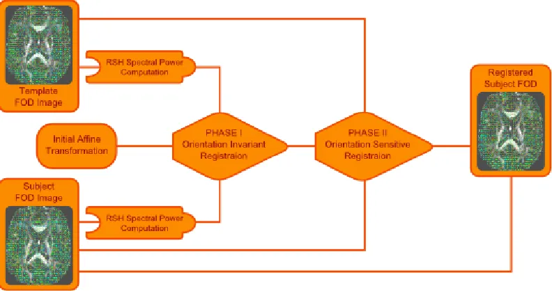
Figure 3.1: FOD registration is accomplished using a two phase registration scheme. First spectral power features are computed and registered. This registration is then improved during a second registration phase where the FODs are directly registered, while reorienting the FOD at each iteration.
utilizes a multichannel Demons registration framework to minimize the difference between the complete FOD images, represented by their RSH coefficients. This representation is dependent on the FOD orientation requiring the finite strain (FS) reorientation method (discussed below) to be used to reorient the FODs at each iteration of the registration pro-cess. The utilization of the two phase process reduces the computational complexity and convergence time, by removing the need to reorient the images in half of the iterations, without sacrificing the accuracy garnered from the inclusion of orientation information.
In phase I, both the fixed and moving images are represented by their RSH spectral power images (discussed in Section B.3) which are rotationally invariant. These images are com-prised of feature vectors of the form vl =
P
m( ˜fl,m)2, where ˜f are the RSH coefficients of the FOD at the particular voxel. The Diffeomorphic Demons framework minimizes the
(a) (b)
Figure 3.2: Images of the posterior corpus callosum, with (a) and without (b) finite-strain reorientation of an FOD image following a 45 degree rotation. Note that without reorien-tation, the principal directions of the FODs do not coincide with the underlying anatomy.
following metric between the moving and fixed FOD images at each voxel,
v u u t
lMax
X
l=0,leven
(X( ˜fl,m)2−
X
(˜gl,m)2)
where ˜f and ˜g are the RSH coefficients of corresponding voxels in F and M.
Phase II uses the full vector of RSH coefficients to represent the FOD at each voxel, mini-mizing the L2 metric in the full RSH space,
v u u t
lMax
X
l=0,leven l
X
m=−l
( ˜fl,m−g˜l,m)2=
Z
dωf(θ, φ)−g(θ, φ) (3.1)
This metric measures the total amplitude difference between the two spherical functions,
f and g, and is inherently sensitive to the orientations of both. Owing to this sensitivity, during the Demons optimization process, we reorient the moving image, using the finite strain reorientation scheme [4], when applying the transformation at the current iteration.
Finite Strain FOD Reorientation
computational simplicity, as well as, its unbiased treatment of the maxima of the data model. Thus at each voxel, the FOD (f) is replaced by f0 =f◦R−1. In the RSH representation, this takes on the form of ˜f0 =Rg−1f˜, where Rg−1 is the matrix representation ofR−1 in the
RSH space, the details of which are discussed in Appendix B.2. The effect and need for performing reorientation can be seen in Figure3.2.
Multichannel Diffeomorphic Demons
The multichannel diffeomorphic Demons algorithm forms the central mechanism that drives both phases of our registration method. It seeks to determine a correction to the current spatial transformation, s, of the form exp(u). This update minimizes a global energy functional defined in terms of the fixed and moving image,F and M,
Es(u) =
X
p∈Ω
||F(p)−M◦s◦exp(u(p))||2L2+
σi
σx
2
||u||2
where p are points in Ω, the domain of the fixed image, F. While the σi
σx term accounts for image noise and interpolation error and acts, as can be seen from equation 3.2, as a regularizer for determining the update field. We can linearize the image similarity term in the region ofu= 0 as:
F(p)−M◦s◦exp(u(p)) =F(p)−M ◦s(p) +Jpu
In the case where F and M are images of vectors, Jp is the Jacobian matrix. With the above linearization, the energy functional simplifies to
Es(u) =X
p∈Ω
F(p)−M ◦s(p) 0 + Jp σi σxI
u(p)
2 L2
equations for each point p.
F(p)−M ◦s(p) 0
+
Jp
σi σxI
u(p) = 0
which simplifies to
(JptJp+
σi
σx
I)u(p) =−Jpt(F(p)−M◦s(p))
yielding following update step
u(p) =−(JptJp+
σi
σx
I)−1Jpt(F(p)−M ◦s(p)) (3.2)
In our application, we have chosen to use the symmetric computation of the Jacobian,
Jp =−Jp(F)+2Jp(M◦s), whereJp(F) andJp(M◦s) are the Jacobians of the fixed and deformed moving images at the point p.
Each iteration of the multichannel diffeomorphic Demons method can be summarized as follows
1. compute an update step uusing equation 3.2
2. smooth u with a Gaussian filter
3. s←s◦u
4. deform the moving image usings
5. apply reorientation if using OS features (Phase II)
This process is repeated either until the update steps no longer substantially reduce the image difference or for a prescribed number of steps.
computed from the fixed and moving images. The resultant transformation is then used as the initial transformation for the second phase, which uses the entire RSH representation of the FOD images and necessitates a reorientation at each iteration.
3.3. Validation: Simulated Experiments
The proposed method was validated by comparing it to each of its constituent registration processes (Phase 1 and Phase 2) as well as to a scalar Demons algorithm that utilizes the non-diffusion weighted (T2 weighted) images from the DW-MRI datasets to drive the registration. These four methods (Phase 1, Phase 2, Combined, T2) were applied to a simulated dataset to evaluate their ability in registering prominent WM structures.
Simulated Datasets
A DW-MRI dataset was acquired on a healthy human using a Siemens (Siemens Medical Systems, Iselin, NJ) Verio 3T scanner and a spin-echo, echo-planar imaging sequence, TE = 106ms, TR = 16.9s, 2mmisotropic voxels,b= 3000 s/mm2and 128 gradient directions with 4 images, with no diffusion weighting (b0). An FOD image, of order 12 (91 components), was computed using the CSD method. This would serve as the template image. A T1 structural image was also acquired. Prominent WM regions of interest (corpus callosum, corona radiata, internal capsule) were determined by registering the template T1 image with the Eve atlas [124]. A WM mask was created using the FSL’s FAST algorithm [198].
T2 Phase I Phase II Combined
R
egi
str
a
tio
n
E
rr
or
(
m
m)
Registration Accuracy
Corpus Callosum Internal Capsule Corona Radiata White Matter
1.2
1.0
0.8
0.6
0.4
0.2
0.0
Figure 3.3: Average displacement error is shown for prominent white matter regions (Corpus Callosum, Internal Capsule, Corona Radiata) and whole brain white matter, for each of the registration methods.
Results
The four registration algorithms (Phase 1, Phase 2, Combined and T2) were then per-formed on these 10 datasets. The resultant deformations were subtracted from the known deformations yielding a displacement error vector at every voxel. The magnitude of the displacement error vectors were then averaged within the ROIs and across subjects.
All methods were robust and produced reliable results for all simulated datasets. Figure3.3
shows the average displacement error within the ROIs and in the whole brain WM. There are three things to note from Figure3.3. First, the inclusion of orientational information (Phase 2 and Combined) improves the registration accuracy compared with the other methods. Second, there is no significant difference between results of the Phase 2 method and the combined method. Finally, the decrease in accuracy when using the Phase 1 method as compared to the T2 method is surprising, although it may be attributed to the fact that the T2 method was used to initially create the simulated datasets.
4th Order 8th Order 12th Order R egi str a tio n E rr or ( m m) Time R at io t o T2 Computation Time Registration Error Phase II Combined 400 100 250 350 300 200 50 150 0 0.170 0.140 0.155 0.165 0.160 0.150 0.135 0.145 0.130
4th Order 8th Order 12th Order
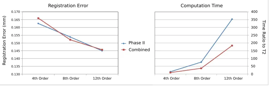
Figure 3.4: A: Average registration error for the internal capsule as a function of the RSH order of the FOD fit. B: Computation time for each registration as a ratio to the T2 registration method.
algorithm. As discussed in SectionB.2, reorientation is a linear operation in the RSH space, and as the dimension of this space, determined by the order of the RSH fit, increases the complexity of determining the reorientation operator also increases. Figure 3.4 shows the average registration error for the internal capsule for the Phase 2 and combined registration methods, as well as the computation time relative to the T2 registration method. The internal capsule was chosen for its small size and thus its susceptibility to registration errors. Even at the lowest order tested (l= 4), we see that both the Phase 2 (0.162mm error) and the combined (0.165 mm error) registration methods out perform the T2 (0.29 mm) and Phase 1 methods (0.8 mm). As the fit order is increased we see a growing separation in computational time between the Phase 2 and combined methods while we see no difference in accuracy improvement between the two. This suggests that it isn’t until the higher order fits (l >4) are being used that the befits of the combined approach be come significant.
3.4. Validation:
In-vivo
Experiments
DW-MRI modalities offer different representations of the same anatomy. Thus, the best
spatial normalization should correctly align both images. The registration algorithms are evaluated based on the their ability to adequately register the DTI, FOD and WM images of the population.
The subjects used for the experiment were the 27 typically developing controls acquired as part of the ASD dataset. A description of this imaging dataset can be found in Section
A.1.1. Both the HARDI and DTI datasets were corrected for Rician noise and eddy current artifact. FOD and DTI images were then fit to their respective datasets. A WM image was determined using tissue segmentation performed on each subject’s structural MP-RAGE image. All three images were then aligned to the FOD image, resulting in co-registered FOD, DTI and WM images for each subject. The details of these procedures can be found in SectionA.2.
Registration Results
For each subject, three spatial transformations are computed, registering their anatomy to that of a 10 year old male chosen to act as a template subject. This process begins with both the FOD and DTI images of each subject being linearly registered to the template space via an affine transformation, computed using the subject’s b0 image. These linearly registered images serve as the starting point for the three registration procedures.
First, the subject’s FOD image is registered to that of the template subject using the proposed non-linear registration process, referred to as FOD-Demons. The DTI image of each subject is then registered into the template space using the DTI-Droid registration algorithm [88] as well as a DTI based version of the Demon’s method presented in Section
3.2, referred to as DTI-Demons. Phase I of the DTI-Demons method uses FA as the rotationally invariant DT feature, while Phase II uses the log-Euclidean [11] representation of the DTs and a finite strain reorientation strategy.
template subject. These deformations are then applied to both the FOD and DTI images of each subject, generating registered images. Residual images, consisting of the voxel-wise difference between the subject’s registered image and the template, are also computed, for each registration method and for each modality. The RSH L2 distance (equationB.5) was used to measure the voxel-wise difference of the FOD images while the Log-Euclidean metric [11] was used for the DTI images.
In addition to computing residual images, population variance images were computed for both the FOD and DTI contrasts, for all three registrations, using equation3.3at each voxel
x, where fi(x) is the model of interest andn is the number of subjects in the population. Again when computing the DTI variance the Log-Euclidean metric was used as the distance measure (d(., .)), while theL2 RSH distance (equationB.5) was used when computing the FOD variance.
V(x) = 1
n
n
X
i
d(fi(x), µ)2 (3.3)
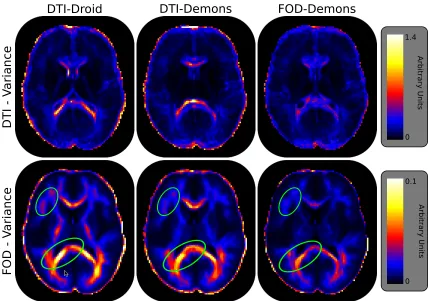
Figure 3.5 shows representative slices of the population variance FOD and DTI images computed using each of the three registration techniques. When examining Figure 3.5it is important to recognize that the FOD and DTI variances are scaled differently since they are computed from inherently different modalities. However, the same scaling is used across the registration types (rows of Figure3.5).
DTI-Droid DTI-Demons FOD-Demons
DTI
V
ar
ian
ce
0 1.4
Arbitr
a
ry U
n
its
FOD
-
V
a
ri
a
n
ce
0 0.1
Arbitr
a
ry U
n
its
Figure 3.5: Representative slices of the FOD and DTI population variance images com-puted for each registration method, DTI-Droid, DTI-Demons and FOD-Demons. Each row is scaled independently since different difference metrics, the Log-Euclidean for DTI and equation B.5 for FOD, are used within equation 3.3 to compute the respective variances. The FOD-Demons registration method is able to minimize both the DTI variance as well as the FOD variance suggesting that it better captures the true anatomical differences between subjects better.
observed using the FOD based technique.
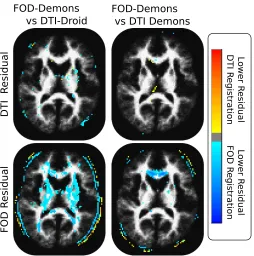
FOD-Demons vs DTI-Droid FOD R esidu al DTI R esidu al FOD-Demons vs DTI Demons
Lo w er R esidu al FOD R egi str at ion Lo w er R esidu al DTI R egist ration
Figure 3.6: Statistical maps determined by four t-tests, performed to identify regions where the registration methods yield different FOD and DTI residuals. Representative slices, thresholded at an FDR correct p-score of 0.001, are shown. The FOD based registration performs significantly better, i.e. yields lower residuals, than either DTI-based technique when the FOD residual is used, while performing similarly when compared on the DTI residual.
A final point of comparison is the ability to register WM volumes of the population. Figure
DTI-Droid DTI-Demons FOD-Demons
White
Ma
tt
er
0 1
Template WM boundary
Figure 3.7: Representative slices of WM masks averaged over the population for each of the registration methods overlaid with the template WM mask (red contour). Higher values in these maps signify a higher degree of overlap in the registered WM masks of the population. Areas where the FOD-Demons registration results in improved alignment of cortical WM structures are indicated in green.
3.5. Conclusions
The general aim of performing spatial normalization, within neuroimaging, is to capture the spatial relationship between the neuroanatomy of different subjects. Once this informa-tion is captured, it can be exploited to either study the geometric (volumetric) differences between the anatomy of individual subjects [13,14,45], or to study the population within
a standard reference frame using other modalities, such as fMRI or DW-MRI. The work
contained in this thesis focuses primarily on examining group differences in regional WM architecture, as represented by diffusion models. Thus we are principally concerned with establishing a correspondence at the voxel level between the WM anatomy of different sub-jects. This necessitates the use of registration techniques that utilized modalities sensitive to differences in WM anatomy, namely those derived from DW-MRI.
model representable in the RSH basis. The method presented is a two phase diffeomor-phic Demons based framework, using an orientation invariant approach in the initial phase followed by an orientation sensitive secondary phase. Simulation studies show that this over-all approach is able to maintain the registration accuracy achieved from the more intensive orientation sensitive method, in reduced computational time (Figures 3.3and 3.4).
Additionally, the proposed method was compared with the DTI-Droid based registration al-gorithm as well as a DTI version of the proposed alal-gorithm (DTI-Demons), in a population of 27 typically developing children. An analysis of both the FOD and DTI population vari-ances (Figure3.5) computed by these techniques indicate that the proposed FOD method is better able to align the anatomy of these subjects, since it better minimizes both forms of variance, while increasing the overlap of cortical WM (Figure 3.7). The FOD-Demons technique is able to significantly (p <0.001) reduce the population residuals (Figure3.6) of the FOD images, when compared to either of the DTI based techniques. However, all the methods were able to adequately reduce the DTI residuals, indicating that by considering the additional information content, available from the FOD modeling, the proposed method is able to better capture the geometric differences in the population.
CHAPTER 4 : White Matter Parcellation
4.1. Introduction
The use of brain atlases in neuroimaging studies allows researchers to register, identify and perform measurements on individual subjects within a common spatial coordinate system enabling large scale group studies. Such studies leverage their greater statistical power to elucidate smaller or more subtle anatomical differences that exist in specific diseases. Since the introduction of the Talairach [162] human cortical atlas, a number of MRI atlases have been introduced to assist with these measurement issues. T1-weighted MRI atlases [12,39,98,97,111,112] have been used extensively to illustrate differences in gray matter anatomy as well as to localize functional signals within these structures. While T1-weighted MRI provides detailed information concerning cortical anatomy, it provides considerably less information concerning white matter anatomy [165], thus these atlases have focused primarily on the identification of GM regions and possess limited detail concerning WM regions.
By providing anin-vivoWM contrast mechanism, DW-MRI has reinvigorated the study of WM pathologies. More recently, DTI-based anatomical atlases [119, 124, 178] have been introduced to address the relative lack of information provided by the existing cortical atlases. While DTI is able to model WM regions possessing a single fiber population, it is ill-suited to model areas of more complex WM, such as fiber crossing. This limitation makes delineating boundaries within these regions difficult and the labeling within them suspect. HARDI data models, such as the FOD, provide contrast in areas of fiber crossing and orientation change that is unavailable from conventional DTI and better reflects the underlying structure of the WM tissue.
region labeling, permits the generation of population/study specific atlases without the need for manual delineation of anatomical regions.
In general, atlases identify spatial regions consisting of voxels that meet some conceptual criterion of sameness. The majority of imaging atlases attempt to label regions based on named neuroanatomical constructs, such as the prefrontal cortex or the internal capsule. This typically requires a neuroanatomist/neuroradiologist to manually label a template im-age to identify each region. A process that is inherently variable, due to the underlying vari-ability of human neuroanatomical boundaries, resulting in different labellings by different neuroanatomists [46,180]. Recent work within the registration community [74,79,80,196] suggests that choosing a registration template from the population under study, improves the accuracy of spatial normalization. However the labor intensive labeling process makes the accurate transfer of atlas defined regions to a population specific atlas difficult, a partic-ularly acute issue when the population has unique characteristics (such as being of a younger age than the anatomical atlas) or when the new imaging modalities, such as HARDI, are being used.
Another important consideration, is whether labeling based on anatomical boundaries pro-vide sufficient demarcation, particularly in areas of complex WM, for applications such as ROI based WM statistical analysis. For instance, most large fiber bundles such as the CC or SLF, sensible targets for anatomical ROI labeling, are known to traverse a variety of WM architectures and thus may not be well suited for ROI studies where they are represented by a single average diffusion model or a single scalar feature derived from the entire region.
homogeneity is the driving force behind the clustering process, each region can be confi-dently represented by its average. This makes these regions ideal for ROI statistical studies or for the extraction of spatial WM features for use in a classification framework.
While neuroanatomical labeling may not provide suitable delineation of boundaries needed to identify homogeneous WM regions, it does aid in interpretability by providing researchers and clinicians with a means of investigating the structure and function of these regions and providing a comparative basis to other published studies. To improve the interpretability of our regions, we assign each homogeneous WM region with neuroanatomical labels based on its spatial overlap with an existing WM atlas. While not designed merely to identify these named anatomical constructs, the neuroanatomical relabeling of the data-based atlas, allows for describing the ROI as belonging to the anatomical region, thereby instilling it with joint information of the underlying fiber orientation as well as the global anatomy and function, thereby facilitating interpretability.
Algorithm 1 Spatially Coherent Normalized Cuts
Require: Initial ROIS: C
Require: N-CUTS parameters: σf,σs
Require: Stopping criteria:
Ensure: Final ROIS: C0
C0 ←C
while maxR∈C0Φ(R)> do
Identify the region,Ci, with the maximal degree of non-uniformity. RemoveCi from collectionC0.
Partition Ci using normalized cuts intoCi,1 and Ci,2.
Extract all the spatially connected regions from bothCi,1 and Ci,2. Add new spatially connected regions to collectionC0.
end while
4.2. White Matter Parcellation
WM regions, that are defined anatomically either based on fiber bundles such as the SLF or the CST, or based on their spatial location such as the internal capsule (IC) or the sagittal stratum (SS) often extend through a range of diverse WM architectures (orientations, cross-ings etc). This heterogeneity is problematic, particularly when using robust WM features such as the DT or the FOD diffusion models in subsequent analysis, as it makes the repre-sentation of these ROIs, by their averages, suspect. These anatomical ROIs are intended to represent anatomical structures and are therefore often not uniform in the feature space of interest. This non-uniformity is the main trait we would like to avoid when defining regions.
To address this, we utilized an approach similar to that of the superpixel [117] methodology. Within this framework, a single WM region or a set of anatomically or otherwise defined regions are iteratively divided into spatially connected subregions, using a normalized-cut clustering routine and a seed growing algorithm to enforce spatial connectedness.
Spatially Coherent Normalized Cuts for WM Clustering
ROIs are supplied as a labeled image, with each label specifying a unique ROI.
The initial step of the algorithm is to parse the supplied labeled image into a collection of fully connected regions. Any region that contains more than one spatially connected component, is divided into those components. This process yields a collection, C, of fully spatially connected regions derived from the supplied labeled image. From C, we identify the region which is most heterogeneous with respect to the FODs it contains. A region’s heterogeneity is represented by the average squared distance (equation 4.1) between the mean FOD (µ) and the FOD (fi) of every voxel in the region. This measure has an interpretation similar to a variance.
Φ(R) = 1
n
X
i∈R
d(fi, µ)2 (4.1)
For the purposes of clustering we utilize the L2 metric on the RSH coefficients of the normalized FODs, equationB.6, to measure the distance between pairs of FODs (d(·)).
![Figure 1.1: Illustrations by Friedrich Arnold [10] of gross dissections of the cerebral hemi-sphere](https://thumb-us.123doks.com/thumbv2/123dok_us/9325475.1467316/14.612.134.520.83.314/figure-illustrations-friedrich-arnold-gross-dissections-cerebral-sphere.webp)
![Figure 2.1: The Stejskal and Tanner pulsed gradient spin echo sequence. Adopted from[185, Westin2002]](https://thumb-us.123doks.com/thumbv2/123dok_us/9325475.1467316/21.612.137.513.86.184/figure-stejskal-tanner-pulsed-gradient-sequence-adopted-westin.webp)