Fuzzy Statistical Process Control of a Calcite Grinding Plant Using Total Color Difference Parameter (Δ E)

ISSN (e): 2250-3021, ISSN (p): 2278-8719

Vol. 07, Issue 05 (May. 2017), ||V1|| PP 07-22

Fuzzy Statistical Process Control of a Calcite Grinding Plant

Using Total Color Difference Parameter (ΔE)

Metin Uçurum

Industrial Engineering Department, Bayburt University. Bayburt-Turkey

Abstract :

-

Statistical process control (SPC) is one of the important approaches used in quality management. SPC can be applied in plants to obtain good quality and high standard products that have become very popular in many industries. Fuzzy process capability analysis by using X-R control charts gives more realistic results, developed with fuzzy theory. Fuzzy control charts are more sensitive than SPC. Therefore, fuzzy control charts lead to producing better-quality products. In this study, total color difference parameter (ΔE) was studied using fuzzy observation on a calcite grinding plant products. For this purpose, color parameters of the grinding plant products were evaluated using triangular fuzzy number (TFN) and fuzzy process capability indices (PCIs). The results show that the mill plant seems to be under control. Therefore, on a randomly selected sample used in the fuzzy statistical process control work was chosen and other color parameters such as whiteness index (WI), saturation index (SI), hue angle (H), browning index (BI) and yellowness index (YI) and particle size properties, XRF, XRD, FTIR, TGA-DTA and SEM were then determined on the calcite sample.

Keywords: Fuzzy Statistical Process Control, X-R Charts, Grinding plant, Total color difference

I.

INTRODUCTION

One of the predominant technologies in mining, production of minerals. and materials treatment is grinding. Ball mills are mainly used for that purpose [1]. Grinding by collision is more effective for size reduction of brittle materials. One of the few machines for grinding of materials by collision is a disintegrating mill-disintegrator [2], a mill for reducing lump material to a granular product. where crushing took place partly by direct impact and partly by interparticulate attrition [3]. Ground and precipitated calcium carbonates are widely used as performance minerals in the rubber, plastics and paper industries. Both untreated and surface-modified forms are used. depending upon the nature of the end product [4].In polymer applications the calcium carbonate is often blended with polypropylene (PP) homopolymer or polyethylene (PE) to improve processability and properties such as stiffness and impact resistance of composite materials. For effective mixing and good adhesion characteristics it is desirable that the surface energies of the mineral and polymer are close to each other [5].

The aspect and color of the calcite surface is the first quality parameter evaluated by consumers and is critical in the acceptance of the product. Industrial applications require specific properties and characteristics. Among the most valuable characteristics is the color, a function of the parent rock and its alteration [6]. In polymineral natural samples with complex crystallochemistry, the study of color is more complicated than in minerals of high purity (or even synthetic ones) where diffuse reflectance spectroscopy techniques are employed [7]. An organization called the Commission International Eclairage (CIE) determined the standard values that are used worldwide to measure color. The values used by CIE are called L*, a*, and b* and the color measurement method is called CIELab. Symbol L* represents the difference between light (where L* = 100) and dark (where L* = 0) a* represents the difference between green (−a*) and red (+a*). and b* represents the difference between yellow (+b*) and blue (−b*) [8].

products obtained as a result of inspections taken randomly from the samples of products in the determined place of the process. The aim of control chart type X-R is to observe and register the changing ability of the characteristics of the researched element of the production process. The example of implementing control chart type X-R shows the possibility of monitoring parameters of the production process according to an idea of defect prevention. Using this method allows monitoring the production process, provides opportunities for cost reduction, and maintains the production process stability [12].

Conventionally, for monitoring a manufacturing process, the Shewhart control charts are applicable on the condition that collected sample data are real-valued numbers only. However. in many cases the key quality characteristic of manufactured products, such as the color-intensity quality of produced pictures or screens and the reading-precise quality shown on analogue measurement equipments, apparently inheres with imprecise character, whose samples data are collected by taking certain imprecise information into consideration, known as interval-valued or fuzzy numbers/data [13,14]. Besides. the fuzzy data may also come from output measurements judging with humans‟ partial knowledge or subjectivity or gathered from the manufacturing process with scarce or coarse samples [15,16,17]. Therefore, based on the fuzzy sample data to identify whether a manufacturing process exists special causes variation, or is needed to makes certain correction. traditional Shewhart control charts must be expanded so as to possibly carry out the process monitoring in this fuzzy environment [18].

In general, statistical and fuzzy methodologies exist to deal with the categorical data. Early research on statistical methodologies goes back to Duncan [19] who introduced a chisquare control chart for monitoring a multinomial process with categorical data. Later. this type of control chart is discussed further by Marcucci [20] and Nelson [21]. Marcucci [20] introduced a statistical approach for the case, where the proportion of each category is not known before. In the case of fuzzy methodologies, several approaches are proposed. Bradshaw [22] for the first time, used fuzzy sets as a basic for explaining the measurement of conformity of each product unit with the specifications.

In this study, data from related color parameters of grinding process products of a company in Niğde-Turkey are obtained. An application is presented for fuzzy X-R control charts; it‟s tried to be analyzed whether or not the process is under control by constructing fuzzy control charts using calculated total color differences (ΔE). In addition, the specifications of the micronized calcite, on a randomly selected sample used in the fuzzy statistical process control work, were then determined by other color parameters such as whiteness index (WI), saturation index (SI), hue angle (H), browning index (BI) and yellowness index (YI) that were calculated and particle size properties of the micronized calcite product were given. In addition, XRD, XRF, FTIR, TGA, DTA analyses were made on the selected ultra-fine grinding sample.

II.

MATERIAL- METHOD

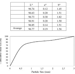
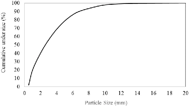
Conventional ball-mill grinding technology is used to obtain calcite with micronized on the industrial scale. Fine/very fine sizes of calcite products could be produced with the mill running closed circuit by separation of air. Flow diagram of a micronized calcite grinding plant is given in Figure 1. The particle size distribution of the mill feed sample was determined by screening. It is shown in Figure 2. It can be seen that the d80 size is about 1.0 mm particle size. The products used in statistical color parameters (L*, a*, b*) studies are cyclone products. In the total color difference calculations, averages of the five samples values, are used as L*=96.77, a*=0.19, b*= 1.56 (Table 1).

Table 1. Color Parameters Values of the Feed Samples

_{L* a* b*}

96.74 0.12 1.45

96.63 0.20 1.51

96.73 0.30 1.82

96.91 0.20 1.50

96.85 0.14 1.51 Avarage _{96.77 0.19 1.56}

Figure 2. Cumulative Under Size (%) of Feed Sample

An organization called Commission Internationale del'Eclairage (CIE) determined the standard values that are used worldwide to measure color. The values used by CIE are called L*. a*. and b*, and the color measurement method is called CIELAB. Symbol L* (Lightness) represents the difference between light (“pure white”) (where L*=100) and dark (“black”) (where L*= 0); a* (Redness-Greenness) represents the difference between green (−a*) and red (+a*); and b* (Yellowness-Blueness) represents the difference between yellow (+b*) and blue (−b*) [8]. The colour measurement method is called CIELAB. The CIELAB values are calculated from the red green and blue filters of the colorimeters and are particularly suited to describing near white samples according to the following equations [24]:

L*= 116 (Y/Yn)1/3-16 (1)

a*=200[((X/Xn)1/3-(Y/Yn)1/3] (2)

b*=200[((Z/Zn)1/3-(Y/Yn)1/3] (3)

where X. Y and Z are the tristimulus values for the samples arising from the colourimetric system and Xn. Yn and Zn are those of a surface colour chosen as the nominal white stimulus. Using this system and colour that correspons to a place on the Cylindrical CIELAB color space system was shown in Figure 3.

Another useful parameter for describing White, which is given in the BS 3900 [26] is delta E (∆Ε). The total color difference (ΔE) was calculated using the measurements and Equation 4. by using L*, a* and b* values [27, 28]. The color parameters (L*, a*, b*) of calcite samples were measured using a Datacolor Elrepho SF450X spectrophotometer in the study.

ΔE = [(L0 − L*)2 + (a0 −a*)2 + (b0 − b*)2]0.5 (4)

where subscript “0” refers to the color reading of the feed sample used as the reference, and a larger ΔE indicates greater color change from the reference sample [24]. The CIELAB, or CIE (1976) L*a*b* values have a perceptual meaning: L* is the lightness which relates to the physical intensity of a color, whilst a* and b* are coordinates on the red–green and yellow–blue color axes respectively. This scheme is designed such that a constant difference in color, ΔE, defined by the Euclidean distance. It should give a constant „perceived‟ total color difference-regardless of the location in the color space. The smallest perceivable difference for two colored patches contacting one another is approximately 0.5–1.0 ΔE units [29]. A whiteness index (WI) has been described based on the distance of a color value from a nominal white point, represented in CIELAB color space as L*=100, a*=0 and b*=0. In spectral terms a white material is one whose reflectance across the visible wave length range is constant and high (i.e. close to 100% or reflectance factor of 1). Varying shades of gray to black have a constant reflectance with the perfect black having a reflectance of 0% [30]. The hue angle is traditionally measured starting at the direction corresponding to pure red. The simplest way to derive an expression for this angle is to project the vector (1; 0; 0) corresponding to red in the RGB (red, green, and blue) space and an arbitrary vector c onto a plane perpendicular to the achromatic axis, and to calculate the angle between them. For the derivation of an expression for the saturation of an arbitrary color c, we begin by looking at the triangle which contains all the points with the same hue as c. The intersection of this triangle and the iso-brightness surfaces are lines parallel to the line between c and its brightness value on the achromatic axis L(c) = [L (c); L (c); L (c)]. Traditionally, the saturation is calculated as the length of the vector from L(c) to c divided by the length of the extension of this vector to the surface of the RGB cube. Moreover, it is clear that this definition of the saturation depends intimately on the form of the brightness function chosen (i.e. on the slopes of the iso-brightness lines) [31]. The Hunter b or CIELAB b* coordinate is often used for the characterization of yellowness. Yellowness indices are unduly neglected in the publications reviewed; they report only in a few cases the application of the according to ASTM (2005), where CX and CZ are illuminant- and observer-specific constants, or the formula 6 often referenced [32]. Browning index in the literature may mean one of two things: a simple indicator of a chemical change (often characterized by the optical density at a given wavelength or the ratio of the reflectance at 570 and 650 nm) or the color change due to oxidation of a freshly cut fruit or vegetable surface, during storage or drying, or the baking of bread. The simplest (and probably least adequate) indicator of the color change is the L* coordinate (or 100 − L* or 100/L*) [33]. Whiteness index (WI), saturation index (SI), hue angle (H), browning index (BI) and yellowness index (YI) were calculated using measured Equation 5, 6, 7, 8 and 9, respectively by using L*, a* and b* values [33, 34, 35]. WI =100 – [(100 − L*)2+ a *2+b *2]0,5 (5)

SI = [a*2+ b*2]0,5 (6)

H = arctan (b*/a*) (7)

BI=[100*(x-0.31)]/0.17 (8)

where; x=(a*+1.75xL*)/(5.645xL*+a*-3.012xb*) YI=142,86xb*/L* (9)

We now briefly review the development of the equations for constructing the control limits on the X and R control charts. In X chart, means of small samples are taken at regular intervals, plotted on a chart and compared against two limits. The limits are known as upper control limit (UCL) and lower control limit (LCL). These limits are defined as below: LCL = - A2*R and (10)

Table 2. Constants for Control Charts [36]

Subgroup size (n) A2 D2 D3 D4

2 1.880 1.128 0 3.267

3 1.023 1.693 0 2.574

4 0.729 2.059 0 2.282

5 0.577 2.326 0 2.114

In these charts, the sample ranges are plotted in order to control the variability of a variable. The centre line of the R chart is known as average range. The range of a sample is simply the difference between the largest and smallest observation. If R1, R2, .... Rk. be the range of k samples, then the average range (R bar) is given by:

= (R1+R2+R3……….Rn)/ki (12)

The upper and lower control limits of R chart are:

Upper control limit: UCLR=D4* (13)

Lower control limit: LCLR=D3* (14) where, factors, D2, D3 and D4 depend only on sample size (n) (Table 2) [37]

Assume that a quality characteristic is defined as "approximately X". Considering the fuzzy sets concept, this value can be converted to the triangular fuzzy number (TFN) = (X1; X2; X3). After measuring a sample of size n from triangular fuzzy numbers (X1j,X2j. ;X3j) j = 1;……….. ; n, the average of this sample can be calculated by extension principle as follows:

(15)

Also considering extension principle. the range of the sample can be calculated by

(16)

=(max X1j, max X2j, max X3j)-(min X1j, min X2, min X3j) (17) =( max X1j- min X1j, max X2j- min X2j, max X3j- min X3j) (18)

where (maxX1j; maxX2j; maxX3j) and (minX1j; minX2j; minX3j) represent the maximum and minimum values of fuzzy measurements, respectively. One method to determine the maximum and minimum values of fuzzy measurements is assign from ranking method [38].

For m subgroups with size n, the fuzzy grand average and the average range of samples are [39]

(19)

(20)

respectively, therefore. the control limits for control charts are calculated as follows:

=( 1+ 2+ 3+ (21)

= =( 1, 2, 3)=(CL( )1, CL( )2, CL( )3) (22)

=( 1- 2- 3- (23) and similarly, for control chart.

=(D4 D4 (24)

= =( 1, 2, 3)=(CL( )1, CL( )2, CL( )3) (25)

=(D3 D3 (26)

centering the process and thus gives no indication of the actual process performance. Kane (1986) [40] introduced index Cpk to overcome this problem. The index Cpk is used to provide an indication of the variability associated with a process. It shows how a process confirms to its specifications. The index is usually used to relate the „„natural tolerances (3r)” to the specification limits. Cpk describes how well the process fits within the specification limits. taking into account the location of the process mean. Cpk should be calculated based on Eqs. (27)–(28) [38, 40, 41].

(27)

] (28)

where μ denotes the process mean. Cpu, l indicates. in addition. how well the distribution is centred about the

nominal (target) value, a property that can better reveal the relationship between the mean and objective values. Assume that specification limits (SLs) and measurements of the considered quality characteristic are

defined by linguistic variables such as „„approximately” or „„around”. Triangular fuzzy numbers (TFNs) are more suitable for this case. SLs can be defined as follows:

(29)

(30)

Also fuzzy process mean and standard deviation can be calculated as follows [42]:

=TFN (µ1, µ2, µ3) (31)

=( , , )=TFN (s1, s2, s3) (32)

Based on these definitions. fuzzy process capability indices can be calculated as follows:

=TFN( ) (33)

=TFN( ) (34)

=TFN( ) (35)

The value of index Cp gives us an opinion about process‟ performance. For example if it is greater than 1.33 which corresponds to 63 nonconforming parts per million (ppm) for a centered process. we conclude that process performance is satisfactory. The six quality conditions and the corresponding Cpvalues are summarized in Table 3 [43].

Table 3. Quality Conditions and Cp Values [43]

Quality conditions Cp values Super excellent 2.00 ≤ Cp

Excellent 1.67 Cp ≤ 2.00 Satisfactory 1.33 Cp ≤ 1.67

Capable 1.00 Cp ≤ 1.33 Inadequate 0.67 Cp ≤ 1.00

Poor Cp ˂ 0.67

On the other hand, steepness ratio can be also defined by the „„steepness factor‟‟ (SF). The SF can be calculated from the PSD curve of the powder using the following equation:

SF =d50/d20 (36)

A curve with the greater than 2 is described as „„broad‟‟ and those with the factor of less than 2 as „„narrow‟‟ or „„steep‟‟ [51].

In this study, the particle size distribution and values of whiteness color parameters (L*, a*, b*) were determined using Mastersizer 2000 (Malvern) and Elrepho 450x (Datacolor) in the laboratory of Mikrokal Co. Nigde-Turkey. Other analyses were performed at Bayburt University. XRD analysis was made between 2-70° by Cu X-ray tube D8 DISCOVER device. TG-DTA and SEM analyzes were performed by using Perkin Elmer STA 8000 and Nova Nano SEM 450 instruments, respectively. The vibration modes of functional groups of the compound were determined by Fourier transforms infrared (FTIR) analysis. The FTIR spectra were measured in the range of 450–4000 cm-1 by the Perkin Elmer Spectrum Two.

III.

RESULTS

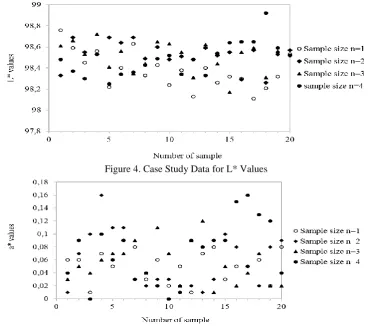
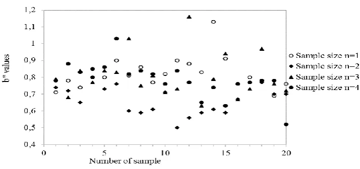
In this study, fuzzy X and R control charts for monitoring the process average and variability based on the fuzzy sample data were given as an example. The appearance of the display seen through total color difference is of great importance for micronized calcite users. For this reason, companies evaluate the amount of total color difference values from feed and ultra-fine calcite products. Color parameters of ground calcite samples are measured with a few grams of sample, obtained from tons of material. Therefore, it seems to be the right approach to use fuzzy statistical methods. At the present time, fuzzy statistical process control methods based upon the product quality data have been the standard approach to process monitoring. In order to analyze the variation in color parameters such as L*, a* and b* (measured using Datacolor Elrepho 450x Datacolor) of the ground calcites delivered to the conventional ball-mill with control charts, data from 20 days have been gathered. Data arranged as m=20 (number of sample) and n=4 (size of sample) are given in the Figure 4, 5 and 6. Calculated values of total color differences (ΔE) using feed and ground samples are given in Table 4.

Figure 4. Case Study Data for L* Values

Figure 6. Case Study Data for b* Values

Table 4. Calculated Values of Total Color Differences (ΔE)

Sample 1 2 3 4

1 2.165 1.769 1.999 1.883

2 1.982 2.097 2.087 1.739

3 1.876 1.999 1.905 1.703

4 1.946 1.915 1.957 1.897

5 1.641 2.095 1.793 1.640

6 1.759 2.033 1.934 1.658

7 2.006 2.150 1.667 1.759

8 1.715 1.979 1.860 1.813

9 1.840 2.066 2.023 1.878

10 1.652 1.914 2.046 1.931

11 1.743 2.042 1.969 1.734

12 1.529 1.806 1.592 1.884

13 1.788 2.068 2.069 1.807

14 1.552 1.995 1.845 1.951

15 1.686 2.027 1.535 2.088

16 1.730 1.762 1.995 2.041

17 1.544 1.968 2.003 2.037

18 1.640 1.693 1.651 2.285

19 1.783 1.959 1.966 1.979

20 1.934 1.995 1.760 2.039

Firstly, a normal distribution test was made with SPSS program. The results showed that the process is said to be normally distributed because the value obtained, 0.457, is larger than α = 0.05 (% 95 reliability level). Therefore, it can be said that the process is normal distribution. In this paper, -R control charts were

Table 5. Total Color Difference as Triangular Fuzzy Numbers (TFNs)

X1 X2 X3 X4

1 2.160, 2.165, 2.170 1.764, 1.769, 1.774 1.994, 1.999, 2.004 1.878, 1.883, 1.888 2 1.977, 1.982, 1.987 2.092, 2.097, 2.102 2.082, 2.087, 2.092 1.734, 1.739, 1.744 3 1.871, 1.876, 1.881 1.994, 1.999, 2.004 1.900, 1.905, 1.910 1.698, 1.703, 1.708 4 1.941, 1.946, 1.951 1.910, 1.915, 1.920 1.952, 1.957, 1.962 1.892, 1.897, 1.902 5 1.636, 1.641, 1.646 2.090, 2.095, 2.100 1.788, 1.793, 1.798 1.635, 1.640, 1.645 6 1.754, 1.759, 1.764 2.028, 2.033, 2.038 1.929, 1.934, 1.939 1.653, 1.658, 1.663 7 2.001, 2.006, 2.011 2.145, 2.150, 2.155 1.662, 1.667, 1.672 1.754, 1.759, 1.764 8 1.710, 1.715, 1.720 1.974, 1.979, 1.984 1.855, 1.860, 1.865 1.808, 1.813, 1.818 9 1.715, 1.715, 1.715 2.061, 2.066, 2.071 2.018, 2.023, 2.028 1.873, 1.878, 1.883 10 1.647, 1.652, 1.657 1.909, 1.914, 1.919 2.041, 2.046, 2.051 1.926, 1.931, 1.936 11 1.738, 1.743, 1.748 2.037, 2.042, 2.047 1.964, 1.969, 1.974 1.729, 1.734, 1.739 12 1.524, 1.529, 1.534 1.801, 1.806, 1.811 1.587, 1.592, 1.597 1.879, 1.884, 1.889

13 1.783, 1.788, 1.793 2.063, 2.068, 2.073 2.064, 2.069, 2.074 1.802, 1.807, 1.812 14 1.547, 1.552, 1.557 1.990, 1.995, 2.000 1.840, 1.845, 1.850 1.946, 1.951, 1.956 15 1.681, 1.686, 1.691 2.022, 2.027, 2.032 1.530, 1.535, 1.540 2.083, 2.088, 2.093 16 1.725, 1.730, 1.735 1.757, 1.762, 1.767 1.990, 1.995, 2.000 2.036, 2.041, 2.046 17 1.539, 1.544, 1.549 1.963, 1.968, 1.973 1.998, 2.003, 2.008 2.032, 2.037, 2.042 18 1.635, 1.640, 1.645 1.688, 1.693, 1.698 1.646, 1.651, 1.656 2.280, 2.285, 2.290 19 1.778, 1.783, 1.788 1.954, 1.959, 1.964 1.961, 1.966, 1.971 1.974, 1.979, 1.984 20 1.929, 1.934, 1.939 1.990, 1.995, 2.000 1.755, 1.760, 1.765 2.034, 2.039, 2.044

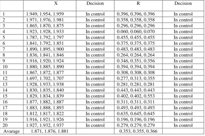
Table 6. Average and Range Values with Control Results

X Decision R Decision

1 1.949, 1.954, 1.959 In control 0.396, 0.396, 0.396 In control 2 1.971, 1.976, 1.981 In control 0.358, 0.358, 0.358 In control 3 1.865, 1.870, 1.875 In control 0.296, 0.296, 0.296 In control 4 1.923, 1.928, 1.933 In control 0.060, 0.060, 0.070 In control 5 1.787, 1.792, 1.797 In control 0.455, 0.455, 0.455 In control 6 1.841, 1.792, 1.851 In control 0.375, 0.375, 0.375 In control 7 1.890, 1.895, 1.900 In control 0.483, 0.483, 0.483 In control 8 1.836, 1.841, 1.846 In control 0.264, 0.264, 0.264 In control 9 1.916, 1.920, 1.924 In control 0.346, 0.351, 0.356 In control 10 1.880, 1.885, 1.890 In control 0.394, 0.394, 0.394 In control 11 1.867, 1.872, 1.877 In control 0.308, 0.308, 0.308 In control 12 1.697, 1.702, 1.707 In control 0.277, 0.313, 0.355 In control 13 1.928, 1.933, 1.938 In control 0.281, 0.281, 0.281 In control 14 1.830, 1.835, 1.840 In control 0.443, 0.443, 0.443 In control 15 1.829, 1.834, 1.839 In control 0.402, 0.402, 0.553 In control 16 1.877, 1.882, 1.887 In control 0.311, 0.311, 0.311 In control 17 1.883, 1.888, 1.893 In control 0.493, 0.493, 0.493 In control 18 1.812, 1.817, 1.822 In control 0.635, 0.645, 0.645 In control 19 1.916, 1.921, 1.926 In control 0.196, 0.196, 0.196 In control 20 1.927, 1.932, 1.937 In control 0.279, 0.279, 0.279 In control

Table 7. UCLX, CLX, LCLX and UCLR, CLR,LCLX Values

X UCLX 2.12 2.13 2.15

CLX 1.87 1.88 1.88

LCLX 1.62 1.62 1.62

R UCLR 0.79 0.8 0.82

CLR 0.35 0.36 0.37

LCLR 0 0 0

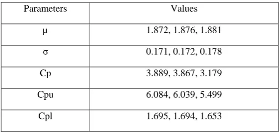
The TFNs of USL and LSL as expected values for calculations indexes were obtained from the management of the plant. Fuzzy process capability indices (PCIs) are determined for the inside total color difference. The measurements in Table 8 are shown as approximate values. Then, the process is checked to determine whether or not it is in statistical control. According to Table 8 and µ, σ, Cp, Cpu and Cpl were obtained by using Equation 26-30 (Table 9). The index Cp, Cpu and Cpl were determined as 3.889-3.866-3.1795, 6.084, 6.039, 5.499 and 1.695, 1.694, 1.653, respectively. The parameters values after performing the few iterations of data collection were greater than 1.33 and it was determined that the plant was adequate for produce coated calcite.

Table 8. Fuzzy Capability Indexes Total Color Difference of Plant

∆E

USL 4.995-5.000-5.005

LSL 0.995-1.000-1.005

Table 9. Values of µ, σ, Cp, Cpu and Cpl Parameters

Parameters Values

µ 1.872, 1.876, 1.881

σ 0.171, 0.172, 0.178

Cp 3.889, 3.867, 3.179

Cpu 6.084, 6.039, 5.499

Cpl 1.695, 1.694, 1.653

Other Color Properties of Randomly Selected Micronized Calcite Product

Table 10. Other Color Parameters Values

Parameters Feed calcite Micronized calcite

ΔE 0 1.91

WI 96.09 98.32

SI 1.57 0.71

H 82.97 97.31

BI 1.76 0.73

YI 1.73 1.03

Particle Size Properties of Randomly Selected Micronized Calcite Product

In this study, cumulative under size (%) of the product, randomly selected sample, are given in Figure 7. The product has d10=0.74, d50=2.84 µm and d90=7.40 µm particle sizes. The size of calcite ore (d50=1 mm) has been reduced to ultra-fine dimensions (d50=2.84 µm) after grinding and separation processes. Table 11 shows some specific particle size, SF, and span values of feed material and final products. The mean particle size of the feed powder as received was approximately 2.84 µm and the steepness ratio was reduced from 3.00 to 2.69. A curve with greater than 2 is described as „„broad,‟‟ and the one with the factor of less than 2 as „„narrow‟‟ and „„steep.‟‟ Expect for one, all of them have smaller values than 2; namely, micronized talc products show broad properties according to SF. In addition, the results of d90/d10, d80/d20 and d90-d10)/d50, PSD width calculations showed that their values decreased with grinding process.

Figure 7. Cumulative Under Size (%) of Randomly Selected Micronized Calcite Product

Table 11. Variation of Some of the Parameters of The Particle Size Distribution with Grinding Time for the Final Product

Meterial SF (d50/d20)

Width of PSD (WPSD)

d90/d10 d80/d20 Span [(d90-d10)/d50)]

Feed 3.00 22.50 8.00 5.73

Some analyses of Randomly Selected Micronized Calcite Product

Chemical properties of micronized calcite sample are reported in Table 12. The analysis indicated that the ore was composed of 99.6% CaCaO3. X-ray diffraction analysis verified that calcite was the sole mineral in the ore (Figure 8).

Table 12. Chemical Properties of Micronized Calcite Sample [52]

Property %

CaCO3 99.60

SiO2 0.01

Al2O3 0.02

FeO2 0.01

MgO 0.20

Others 0.16

Total 100

Figure 8. X-ray Diffraction Analysis of Randomly Selected Micronized Calcite Product

Figure 9. TG and DTA Analysis of Randomly Selected Micronized Calcite Product

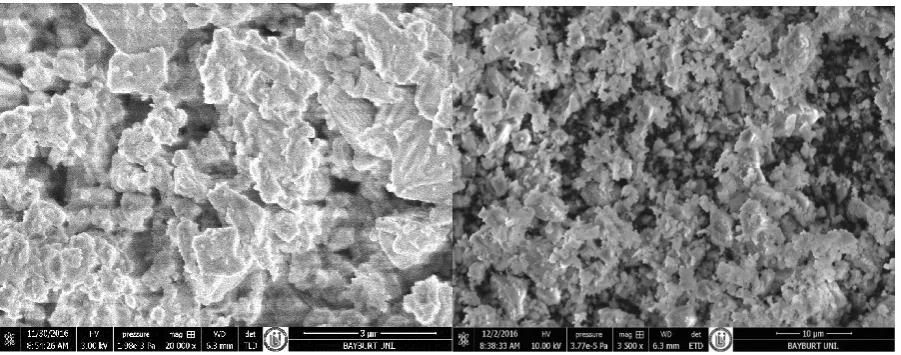
Scanning Electron Microscopy (SEM), also known as SEM analysis or SEM microscopy, is used very effectively in microanalysis and failure analysis of solid inorganic materials. Scanning electron microscopy is performed at high magnifications, generates high-resolution images and precisely measures very small features and objects [55]. Figure 11 shows scanning electron microscopy (SEM) images of micronized calcite. It can be seen that the surface of calcite after grinding appears smooth and uniform.

Figure 10. FTIR Analysis of Randomly Selected Micronized Calcite Product

IV.

CONCLUSION

The results acquired from this study which aims the fuzzy process controlling of the relevance of a calcite grinding plant using color difference parameter (ΔE) of a commercial foundry are summarized below;

i) The process variations have to be controlled using fuzzy statistical process control and process capability index that is one of the important aspects in any production line. X-R control charts created with c o l o r d i f f e r e n c e were observed to be in control. In addition, the calculated Cp values such as 3.889-3.867-3.179, are greater than 1.33. Meanwhile, the Cpru and Cprl values are greater than 1.33. Therefore, it can be said that the process is adequate.

ii) Total color difference (ΔE), which is a combination of parameters L*, a* and b* values, is a colorimetric parameter extensively used in the micronized calcite products to characterize the variation of colors depending on processing conditions. An increase in ΔE was observed with the grinding operation from 0 to 1.91. Experimental results are shown which indicate significant increase from 96.09 to 98.32 for WI with grinding process. As seen in the same table, the saturation index (SI) decreased from 1.57 to 0.71. In addition, on hue angle (H), values increased important ratio from 82.97 to 97.31. Besides these, significant reductions were obtained in BI and YI color parameters with calcite ore grinding.

iii) In this study, cumulative under size (%) of the product, randomly selected sample has d10=0.74, d50=2.84 µm and d90=7.40 µm particle sizes. The mean particle size of the feed powder as received was approximately 2.84 µm and the steepness ratio was reduced from 3.00 to 2.69. A curve with greater than 2 is described as „„broad,‟‟ and the one with the factor of less than 2 as „„narrow‟‟ and „„steep.‟‟ Expect for one, all of them have smaller values than 2; namely, micronized talc products show broad properties according to SF. In addition, the results of d90/d10, d80/d20 and d90-d10)/d50, PSD width calculations showed that their values decreased with grinding process.

iv) FTIR analysis showed that there is a normal result for calcite. DTA results show that there was no an exothermic reaction in the calcite. TG curves demonstrate that the calcite has a layer situation. Electron microscopy (SEM) images of micronized calcite show that the surface of the calcite after grinding appears to be smooth and uniform.

v) The fuzzy statistical process control methods are very effective in the grinding plant of calcite.

V. ACKNOWLEDGEMENTS

The author wish to thank Nidaş limited company, Nigde/TURKEY and to their colleagues who participated and provided support in the work.

REFERENCES

[1]. T.W. Chenje, D.J. Simbi, E. Navara, Relationship Between Microstructure, Hardness, Impact Toughness and Wear Performance of Selected Grinding Media for Mineral Ore Milling Operations, Mater. Des. 25, 2004, 11–18.

[2]. B. Tamm, A. Tymanok, Impact Grinding and Disintegrators, Proc. Estonian Acad. Sci. Eng. 2/2 (1996), 209–242.

[3]. P. Kulua, R. Tarbea, H.D. Kaerdi, Abrasivity and Grindability Study of Mineral Ores, Wear, 267 (2009), 1832–1837.

[4]. Katz. H. S. and Milewski. J. V. Eds.. Handbook of Fillers and Reinforcement for Plastics Van Nostrand-Reinhold. NY. 1978.

[5]. H.P. Schreiber, J.M. Viau, A. Fetou and Z. Deng, Some Properties of Polyethylene Compounds with Surface-Modified Fillers, Polym. Eny. Sci. 30 (5), 1990, 263-269.

[6]. H. Murray, Industrial Clays Case Study. Report of the Mining. Minerals and Sustainable Development Project, International Institute for Environment and Development and World Business Council for Sustainable Development, 2002, 64.

[7]. R.G.Burns, Mineralogical Applications of Crystal Field Theory, Cambridge Topics in Minerals Physics and Chemistry, Second Edition, Cambridge Univ. Press. Cambridge, (1993).

[8]. R. Sharafudeen, The Manufacturing Process Parameters Affecting Color and Brightness of TiO2 Pigment, Int. J. Ind. Chem, 3, 2012, 1-7.

[9]. K. Theodora, L. Jennifer, F.M. John, Experiences with Industrial Applications Of Projection Methods for Multivariate Statistical Process Control, Computers Chem. Eng. 20, 1996, 745-750.

[11]. W.H Woodall, Controversies and Contradictions in Statistical Process Control, J. Qual. Technol. 32, 2000, 341-350.

[12]. M. Dudek-Burlıkowska, Using Control Charts X-R in Monitoring a Chosen Production Process, J. Achieve. Mater. Manufactur. Eng. 49, 2011, 487-498.

[13]. R. Filzmoser, R. Vertl, Testing Hypotheses with Fuzzy Data: The Fuzzy Pvalue, Metrika. 59, 2004, 21– 29.

[14]. R. Viertl, D. Hareter, Fuzzy Estimation and Imprecise Probability, Journal of Applied Mathematics and Mechanics, 84, 2004, 731–739.

[15]. M. Gülbay, C. Kahraman, An Alternative Approach to Fuzzy Control Charts: Direct Fuzzy Approach, Information Sciences, 177, 2007, 1463–1480.

[16]. A. Kanagawa, F. Tamaki, H. Ohta, Control Charts for Process Average and Variability Based On Linguistic Data, International Journal of Production Research, 31, 1993, 913–922.

[17]. N. Sugano, Fuzzy Set Theoretical Approach to Achromatic Relevant Color on The Natural Color System. International Journal of Innovative Computing, Information and Control. 2(1), 2006, 193–203.

[18]. M.H. Shu, C.W. Hsien, Fuzzy X And R Control Charts: Fuzzy Dominance Approach, Computers & Industrial Engineering, 61, 2011, 676–685.

[19]. A. Duncan, A Chi-Square Chart for Controlling a Set of Percentages, Industrial Quality Control, 7, 1950, 11–15.

[20]. M. Marcucci, Monitoring Multinomial Processes, Journal of Quality Technology. 17, 1985, 86–91. [21]. L.S. Nelson, A Chi-Square Control Chart for Several Proportions, Journal of Quality Technology, 19,

1987, 229–231.

[22] C.W. Bradshaw, A fuzzy Set Theoretic İnterpretation of Economic Control Limits, European Journal of Operational Research, 13, 1983, 403–408.

[23]. A Brief Introduction to Neural Networks. Available at http://www.varlikmakina.com/kompletesisler (accessed on May 20 st., 2010).

[24]. G.E. Christidis, N. Sakellariou, E.M. Repouskou, Influence of Organic Matter and Iron Oxides on the Colour Properties of a Micritic Limestone From Kefalonia, Bulletin of the Geological Society of Greece vol. XXXVI (2004), 72-79.

[25]. M.D. Fairchild, Color Appearance Models. Reading, Mass: Addison Wesley Longman, Inc. (1998). [26]. British Standards Institution-BS3900. Parts D8. D9 and D10, Determination of Colour and Colour

Difference: Principles, Measurement And Calculation, (1986).

[27]. M. Maskan, Kinetics of Color Change of Kiwifruits During Hot Air and Microwave Drying, Journal of Food Engineering, 48(2), 2001, 169-175.

[28]. R.C.L. Homco, K.J. Ryan, S.E. Wicklund, C.L. Nicolalde, S. Lin, F.K. Mckeith, Effects of Modified Corn Gluten Meal On Quality Characteristics of a Model Emulsified Meat Product, Meat Science,67, 2004, 335-341.

[29]. A. Joiner, I. Hopkinson, Y. Deng, S. Westlan, Review of Tooth Colour and Whiteness, Journal of Dentistry, 2008, 365.

[30]. C. Saricoban, M.T. Yilmaz, Modelling the Effects of Processing Factors on the Changes in Colour Parameters of Cooked Meatballs Using Response Surface Methodology, World Applied Sciences Journal, 9(1), 2010, 14-22.

[31]. A. Hanbury, The Taming of the Hue, Saturation and Brightness Colour Space, The Seventh Computer Vision Winter Workshop was held onFebruary, 2002, 4–7.

[32]. F.J. Francis, F.M. Clydesdale, Food Colorimetry: Theory and Applications, Westport, CN: AVI Publishing, (1975).

[33]. R. Hirschler,Color in Food, Technological and Psychophysical Aspects, CRC, 2012, 93–104.

[34]. M. Maskan, Kinetics of Colour Change of Kiwifruits During Hot Air and Microwave Drying, Journal of Food Engineering, 2001, 48.

[35]. R.C.L. Homco, K.J. Ryan, S.E. Wicklund, C.L. Nicolalde, S. Lin, F.K. Mckeith et al., Effects of Modified Corn Gluten Meal On Quality Characteristics of A Model Emulsified Meat Product, Meat Science, 2004, 67.

[36]. A Brief Introduction to Neural Networks. Available at http://www.bessegato.com.br/UFJF /resources/table_of_control_chart_constants_old.pdf (accessed on November 29 st., 2016).

[37]. D.R. Prajapati, Implementation of SPC Techniques in Automotive Industry: A Case Study, International Journal of Emerging Technology and Advanced Engineering, 2(3), 2012, 227-241.

[38] . D.C. Montgomery, Introduction to Statistical Quality Control, New York: John 626 Wiley & Sons, (2005)

[40]. V.E. Kane, Process Capability Indices, Journal of Quality Technology, 18, 1986, 41–52.

[41]. S. Kotz, N. Johnson, Process Capability Indices – A review 1992–2000. Journal of Quality Technology, 34, 2002, 2–19.

[42]. I. Kaya, C. Kahraman, Process Capability Analyses Based on Fuzzy Measurements and Fuzzy Control Charts, Expert Systems with Applications, 38, 2011, 3172–3184.

[43]. C.C. Tsai, C.C. Chen, Making Decision to Evaluate Process Capability Index Cp with Fuzzy Numbers, International Journal of Advanced Manufacturing Technology, 30, 2006, 334–339.

[44]. H. Karbstein, F. Muller, R. Polke, Producing Suspensions with Steep Particle Size Distributions in Fines Ranges, Aufbereitungs-Technik 36, 1995, 464–473.

[45]. H. Karbstein, F. Muller, R. Polke, Scale-up for Grinding in Stirred Ball Mills, Aufbereitungs-Technik, 37, 1996, 469–479.

[46]. A.D. Salman, C.A. Biggs, J. Fu, I. Angyal, M. Szabo, M.J. Hounslow, An Experimental Investigation of Particle Fragmentation Using Single Particle Impact Studies, Powder Technology, 128, 2002, 36–46.

[47]. D.A. Gorham, A.D. Salman, M.J. Pitt, Static and Dynamic Failure of PMMA Spheres, Powder Technology, 138, 2003, 229–238.

[48]. G. Matija, S. Kurajica, Grinding Kinetics of Amorphous Powder Obtained by Sol–Gel Process, Powder Technology 197, 2010, 165–169.

[49]. Karbstein H, Muller F, Polke R. Scale-up for grinding in stirred ball mills. Aufbereitungs-Technik. 1996:37:469–479.

[50]. M. Nakacha, J.R. Authelina, A. Chamayoub, J. Dodds, Comparison of Various Milling Technologies for Grinding Pharmaceutical Powders, International Journal of Mineral Processing 74, 2004, 173–181. [51]. H. Adi, I. Larson, P. Stewart, Use of Milling and Wet Sieving to Produce Narrow Particle Size

Distribution of Lactose Monohydrate in The Sub-Sieve Range, Powder Technology, 179, 2007, 95–99. [52] A Brief Introduction to Neural Networks. Available at

http://nidas.com.tr/index.php?option=com_content&view=article&id=48&Itemid=55 (accessed on November 30 st., 2016).

[53]. K.A.R. Gomari, A.A.Hamouda, R. Denoyel, Influence of Sulfate Ions on the Interaction Between Fatty Acids and Calcite Surface, Colloids Surf. A: Physicochem. Eng. Aspects, 287, 2006, 29-35.

[54]. S.D. Cifrulak, High-Pressure Mid-İnfrared Studies of Calcium Carbonate, Amer. Mineral, 55, 1970, 815-824.