WWJMRD 2019; 5(2): 58-65 www.wwjmrd.com
International Journal Peer Reviewed Journal Refereed Journal Indexed Journal
Impact Factor MJIF: 4.25
E-ISSN: 2454-6615
Benedicto Kazuzuru
Senior lecturer, Department of Mathematics, Informatics and Computational Sciences, College of Science and Education, Sokoine University of Agriculture, Tanzania
Correspondence:
Benedicto Kazuzuru
Senior lecturer, Department of Mathematics, Informatics and Computational Sciences, College of Science and Education, Sokoine University of Agriculture, Tanzania
Determinants of Tanzania Exports: A Panel Data
Regression Approach.
Benedicto Kazuzuru
Abstract
One of the major problems among developing countries including Tanzania is the persistence negative balance of trade and balance of payment which results into lack of foreign currency to finance imports. In Tanzania a number of scholars have addressed this problem by finding ways to boost export performance. Unfortunately, over the years dominant studies on export performance particularly in Tanzania have been mainly time series studies which of course suffer from the fact that African countries including Tanzania have no adequate time series data. The most that an African country could have in time series data is a series of 60 years (from independence to the present time). On top of this problem time series estimates might be inconsistent as they cannot safe guard a model from omitted variables. This study employed panel data model in explaining determinants of Tanzania exports. Panel data provides more data points and they are somewhat immune to problems of omitted variables. The proposed determinants were lagged export value, FDI’s, Tanzania GDP; partner Country GDP, Distance, real exchange rate, and dummies for regional economic integration (SADC and EAC). The results indicate all the variables to be significant in explaining exports except real exchange rates. It is recommended to the government of Tanzania and to other stake holders to actively promote foreign direct investments, to handle the oversee customers with a great care, promoting exports to the oversee through its organs such as TANTRADE, and improving the Tanzanian GDP through rapid industrialization and through agriculture improvement.
Keywords:Exports, Panel data, Gravity model
1. Introduction
The importance of exports on a country’s economic growth is unquestionable. Export growth can enhance economic growth through proper utilization of the revenue accrued through exports. A number of authors such as Basu et al (2000), Fosu (1990) and Giles and Williams ( 2000) have acknowledged the importance of exports in a country’s economic development. Improving export performance is one of macroeconomics objectives of many countries including both developing and developed ones. This is because export plays a vital role in economic growth and the means for improving the current account balance. The real export has a positive effect on economic growth in short run as well as in long run. Growth in export may lead to greater productive efficiency through economies of scale or technical improvements as a result of contact with foreign competitors (Chemeda, 2001).
In its effort to increase export supply capacity, Tanzania adopted Liberalization policies in the early 1990s. The country implemented a number of reforms in order to reorient country`s economic policies towards an export-oriented growth strategy. These included establishment of the export processing zones, joining multilateral and regional trading blocs including the Southern Africa Development Community (SADC), the East African Community (EAC), the African Growth and Opportunity Act (AGOA), the World Trading Organization (WTO) and the Economic Partnership Agreements (EPA). This was just to increase access to external market and promote export with the anticipation that the investors in Tanzania will enjoy the expanded market as well as preferential treatments for their products
The role of economic reforms and policies adopted in promoting Tanzania`s export can be confirmed by the fact that total exports of goods and services in Tanzania have been increasing. The improvement has mainly been driven by increase in travel (tourism)
receipts, manufactured goods and gold. Travel maintained the leading position among the foreign currency earners before manufactured goods, gold and traditional export with USD 2,267.4 million worth of export in the year ending September 2016 showing a year on year increase of 12.8%. Foreign exchange earnings from manufactured goods increased by 5.02% to USD 1,330.9 million in the
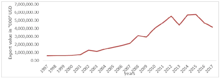
year ending September 2016 with notable improvement recorded in edible oil, textile apparels, plastic goods, and fertilizer and paper products (BOT, September 2016). Figure 1 shows trends in merchandize exports from 1997 to 2017 while figure 2 shows Tanzania major importing countries.
Fig.1: Trends in Tanzania’s Merchandize Exports from 1997 to 2017 Source: Author drawing using statistics from the World Bank
Fig.2: Tanzania’s Average Exports to Major Importing Countries (1997-2017) Source: Author drawing using statistics from the World Bank
The share of Tanzania exports in the world trade has been on the decline. The nation maintained a surplus balance of trade up to 1969 but has experienced a widening trade deficit since then. Throughout most of the 1990s, Tanzania’s trade performance was comparatively stable. Annual exports were of an order of US$ 0.6-0.7 billion, imports around US 1.5-1.7 billion, thus resulting in a current account deficit in the region of US$ 1 billion per year. Essentially this deficit has been financed by disbursements of official development assistance which have climbed steadily over the past decade to now reach some US$ 1 billion per year (Ministry of Industry and Trade, 2009).
To improve this situation Tanzania implemented a number of trade and fiscal policy reforms since the mid – 1980s as the way to promote export by providing a number of incentives. Some of these incentives include abolishing export taxes licenses as well as subscribing to number of preferential trade arrangements and treaties that provide a
fair access to foreign market opportunities (Milanzi, 2012). However, export performance has not been satisfactory. This is from the fact that Tanzania has never experienced trade surplus since 1970s (Sayuni, 2006)
Understanding why this is the case require empirical research effort to determine the root cause of poor export performance. Various research efforts have been done in developing countries including Tanzania to explain determinants of export performance for example Musinguzi and Obwana (1999) found that export growth rate is significantly affected by terms of trade. Ngeno (1996) found that output and real exchange rate affect export rate while Paulino (2002) observed that foreign direct investments significantly affects exports volumes. On contrary Nimrod (2006) found that foreign direct investments and real exchange rate do not explain export growth rate.
However, most studies on export performance in Tanzania such as Rwenyagila (2013) and Manamba 2016) are based on time series analysis which for the case of developing countries including Tanzania there is inadequate data to support it. This study would employ panel data analysis which provides more data points than time series analysis. The advantages of using panel data models is that it can consistently estimates effect of the proposed variables on export performance using fixed effect models, unlike in time series or cross-sectional data where such estimation is not possible.
Another advantage of using panel data models is that it can provide the extent to which export performance is influenced by both unobservable countries’ specific effects as well as by time variation effect, something which cannot be captured in time series models. For example, with panel data model it is easy to capture effects of economic integration and historical relationship on a country’s export performance. Specifically, the study intends to do the following:
(i) To examine the influence of historical
relationship and economic integration on export performance in Tanzania.
(ii) To examine the role of a country’s loyalty to her trading partners
Finding of this study will help the policymakers to come up with the appropriate policy regarding the growth of the sector and the economy as whole, especially because consistent estimates will be made using fixed effect models, something which is not possible in time series models or cross-sectional models.
2.0 Literature Review
2.1 Theoretical literature Review
The principal objectives of any theory of international trade are to explain cause and pattern of trade. Two other objectives of theory of international trade are to explain the composition and volume of external trade. A theory which explains these three issues; cause composition and volume of trade is said to be theory of international trade (Appleyard et al., 2010). These theories have evolved over time along with developments in economic thought; starting with the earliest protectionism view, dominant in the mercantilist era, up to the recent gravity model theory (Mjema, 2004). Salvatore (2010) puts these international trade models chronologically into five main categories, capable of explaining the pattern of trade as follows: First is the Adam Smith absolute advantage theory, which asserts that when one nation is more efficient than(or has an absolute advantage over) another in the production of one commodity, but is less efficient than(or has an absolute disadvantage with respect to) than the other nation in producing a second commodity,then both nations can gain by each specializing in the production of the commodity of its absolute advantage and exchanging part of its output with the other nation for a commodity of its absolute disadvantage.
Second is the Ricardian comparative advantage theory, which asserts that even if one nation is less efficient than (has an absolute disadvantage with respect to) the other nation in the production of both commodities, there is still a basis for mutually beneficial trade. According to the theory, the movement of goods and services between nations is
caused by the comparative advantages which nations have in the production of different commodities.
Third is the Hescscher- Ohlin theory. This theory differs from the former as it considers comparative advantage in terms of factor endowments. According to the theory, countries will export goods that make intensive use of locally abundant factors, and import goods that make intensive use of locally scarce factors.
Fourth is the new trade theory, which tries to explain several facts about trade, which the previous models have had difficulty with. These include the fact that most trade is between countries with similar factor endowments and productivity levels and a large amount of multinational production (i.e. foreign direct investment) characterizes this approach.
Fifth is the gravity model theory. The model, in its basic form predicts trade based on the distance between countries and the interaction of the countries’ economic sizes. The model has been borrowed from the Newtonian law of gravity, which also considers distance and physical size between objects, as the factors for attraction. The model has proved to be strong through econometrics analysis. The physical size in the contest of international trade usually refers to the countries’ GDP. Distance represents the actual distance and all other factors such as transport costs, Real exchange rates and FDI’s which would hinder or smoothen the trade between trading partners. This study would also employ gravity model theory in explaining the factors influencing Tanzanian exports.
2.2 Empirical literature Review
The performance of a country’s exports is highly dependent on its exchange rate regime
and more specifically the real exchange rate. Various studies have shown that the
demand for a country’s exports increases when its export prices fall in relation to the
world prices. The depreciation of its currency compared to other currencies particularly
the dollar, makes its exports cheaper on the international market. For example, Sharma (2001) discovered that the demand for Indian exports increased when its export prices fell. The study also shows that the application of the Indian rupee at one time adversely
affected Indian Exports. In Uganda, Kasekende and Atingi-Ego (1999) found no significant relationship between real exchange rate and export volumes.
In Tanzania, Ndulu and O'Connell (1999) conducted a time series study on non-traditional Exports (NATE) whereby they found a positive significant relationship between real exchange rate, devaluation and export growth on NATEs.In a related study, Jorgen and Michel (2008) in Tanzania using a gravity model found that the real exchange rate did not have a significant impact on Export. Sayuni (2006) on “Determinants of Trade Balance in Tanzania 1970 to 2002” found that real exchange rate had a negative impact on trade balance, meaning that currency devaluation is not the solution for export promotion.
export performance indirectly through the increased access to important raw materials”
A more comprehensive study on African countries was given by Mold and Prizzon (2008), who used a dynamic panel data set for forty-eight African countries over the period 1987 –2006 to identify the key determinants of export performance. The results from the pooled
regression revealed that unit price of exports, real effective exchange rate, taxes on trade
and diversification index to affect export volumes negatively and significantly while
income per capita, and share of manufacturing in GDP and FDI inflows as a percentage of GDP to affect export volumes positively and insignificantly.
Dijk, (2002), conducted a study in Indonesia and found that Foreign Director Investment was very significant in explaining its export performance.
Analogously, Paulino (2002) while studying effect of trade liberalization in
selected 48 developing countries found that foreign direct investment has significant
impacts on export volumes. Agasha (2007) revealed that foreign direct Investment sometimes choose sectors in the economy where a country may not have relatively specialized and this also affect export performance. Also, the study suggested that imports of intermediate inputs and machinery are important determinants of changes in the export performance.
Exportation and value of trade between two countries can be determined by countries GDP and the distance between two countries. Assuming that trade is proportional to the products of the two countries GDPs and inversely proportional to the distance (Krugman et al., 2012). More studies find that internal factors are vital components in improving the export performance of a country concern (Abolagba et al., 2010). Evidences also indicates that by improving internal factors such as production capacity, infrastructure and availability of agricultural products help increasing the export performance. Indeed, internal factors are supported by empirical evidence to influences export performance (Kingu, 2014) whereas few other studies observe that export performance are influenced by external factors (Kusi, 2002)
Devaluation or depreciation of domestic currency has positive contribution to export performance since it makes the price of exported commodities cheaper and increase the volume of commodities (Kingu, 2014). Paulino and Thirlwall (2004) find that when the income of the trade partners improves it also increase export performance of the commodities. In another account good trade policy results in higher export performance of a country and help improving the supply chain mechanism within the country. (Gbetnkom and Khan, 2002)
2.3 Summary of the Literature Review and knowledge gap
It had been observed that some of the reviewed empirical studies, despite of using
different approaches their results converge while some of them contradict each other. For
instance most of the findings support the notion that FDI has a positive influence on
export performance. However, Menji(2010)) and Nimrod (2006) found no support for this
contention. Similarly, Neeru et al (2006), Ndulu and O'Connell (1999) found a positive significant relationship between real exchange rate and export performance. On the other hand, Kasekende and Atingi-Ego (1999) as well as Jorgen and Michel (2008) their studies had found a negative relationship between real exchange rate and export performance.
More important is that few of the mentioned studies could address country specific characteristic such as being a member of a particular regional block or having historical ties with an exporting country because the studies used time series data. Also, few of these studies have investigated the effect of current exports on the future exports. These two gaps have been captured in this study.
3. Methodology
3.1 Study Design, Sample Size, Data Collection
As proposed in section 2, the study used panel data design. 99 countries that are trading partners to Tanzania were considered from the year 1997 to 2017 making a sample size of 2079 data points. All the data sources were secondary sources obtained from various websites as detailed in section 3.5.
3.2 The Estimation Model
Based on the reviewed literature and using the gravity model theory as explained in section 2.1 the study proposes the following model to explain export performance in Tanzania.
EXit=βo + β1EXit-1 +β2FDIt +β3TGDPt+ β4PGDPit+
β5DISTi + β6REXit + β7SADC +β8EAC+ εit --- (1)
Where
EXit is the export value in year t to country i
measured in thousands of USD
EXit-1 is the value of last year exports to country
i in year t
FDIt is the value of foreign direct Investment
which Tanzania received in year t TGDPt is the value of Tanzania GDP in year t
measured in billions of USD
PGDPit is the trading partner income proxied as a
partner GDP per capita measured in USD DISTi is the distance from Tanzania to a country
i measured in terms of kilometers
REXit is the real exchange rate between
Tanzanian and the partner country i, in year t measured as a partner country price of buying a unit of Tanzanian shilling SADC is dummy for a country being either in
SADC and is equal to 1 if a country belongs
to such the regional block and is 0 if otherwise. This dummy will also capture the influence of historical ties between Tanzania and countries in the SADC block which were forming the movement for liberation struggles of countries in the southern region
EAC is a dummy for a country being in East African Community and is equal to 1 if a country is in East African Community and is 0 if otherwise
The variables in the proposed equation have both time dimension and cross-section dimension implying a panel data consideration as suggested in the previous section. In order to interpret the coefficients as elasticities, as preferred in demand studies and also to avoid the impact of highly likely abnormality of observations such as exports and partner country GDP per capital, the study adopts the double logarithmic function model. The use of logs of the variables instead of the variables themselves reduces the extremely huge values into moderate ones, without reducing much the smaller ones, because the logarithmic function increases at a declining rate (Kazuzuru, 2012), accordingly, one can rewrite equation (1) in a more detailed form as
εit ----(2)
Where the variables are as defined before and they enter the model in their natural logs except the dummies.
3.3 An overview of Panel data Modelling
Panel data as said involve both time and cross-section dimensions. When a lagged dependent variable is included as one among the independent variables as in this study one gets dynamic panel data model while when it is not included one get static panel model.
In the static panel modelling there three models under consideration, pooled OLS, Fixed effect model and Random effect model. The pooled OLS assumes that the unobservable individual specific effects (in this case unobservable country specific effects) do not exist. This assumption is not realist. The fixed effect model assumes that such country specific effects exist and usually a one-way ANOVA is used to confirm the existence of country specific effects. To remove country specific effects, it regresses first difference of the dependent variable against the first difference of the independent variables. An alternative approach is using fixed effect within model which regress the difference between a dependent variable and its time average against the difference between independent variables and their time averages.
The random effect model also assumes that country specific effects exists but they are uncorrelated with the regressors in the current model, thus there is no need of removing them. Therefore, comparatively the fixed effect model is taken to be a consistent model (free from confounding variables) whereas a random effect model might be
consistent or inconsistent depending on the validity of its assumption. To establish whether a random effect model is consistent, a hausman test is usually employed to compare the coefficients of the two models.
The static panel model techniques (Fixed and random effect) cannot be used under a dynamic panel model because they would yield inconsistent estimates due to the inclusion of lagged dependent variable in the model. Also, there is a problem of variables not being stationery. To avoid these problems the model in equation 2 is normally restated as follows with variables in their first difference.
---- (3)
The lagged dependent variable
would likely correlate with the differenced error term leading to inconsistent estimates. Anderson and Hsiao (1982) propose using
as an instrument for because
is directly correlated with and uncorrelated with the error term (Cameron and Trived, 2005). However, to get efficient estimates one has to use all possible lags of the instrument variable. Arrelano and Bond (1991) proposed a generalized method of moments (GMM), which uses all possible lags of the dependent variable as instruments for
TA
it1(Cameron and Trived, 2005). This method yields both consistent and efficient estimates, incase its key assumptions are fulfilled (Kazuzuru, 2012)The first key assumption is the absence of second order serial correlation in the equation (9). The fulfillment of this assumption guarantees .The second crucial assumption is the exogeneity of the instruments used in GMM. The instruments cover the lagged dependent variables as well as the lagged predetermined variables. The GMM estimator in Stata provides the test for the two assumptions. The test for exogeneity of the instruments is known as the Sargan test for overidentifying restrictions. In both tests acceptance of the null hypothesis guarantees the consistency of the GMM estimates (Kazuzuru, 2012) It should be noted that all dummies do not appear in equation 3, because their difference is zero. In other words, the dummies would not be estimated in a dynamic panel model but only in a random effect model.
3.4Priori Direction of the Relationship Between Export Value and the Explanatory Variables
Table 1: Expected Signs of the Explanatory Variables
variable acronym Direction
Value of last year exports Indeterminate
Foreign Direct Investment FDIit +
Tanzania annual GDP TGDPt +
Partner Country GDP per capita PGDPit +
Distance between Tanzania (DSM) and the tourist country’s capital DISTi -
Real Exchange rate between Tanzania and a partner country Rex -
Dummy for a partner country being a member of either SADC or COMESA SADC&COMESA +
Dummy for a partner country being in EAC Border +
3.5 Variables and Data Sources 1. Export values
This was obtained from World Integrated Solution website which was developed by the World Bank in consultation with UNCTAD, UNSD and WTO. The website is given as
https://wits.worldbank.org/CountryProfile/en/Country/TZA/ Year/LTST/TradeFlow/EXPIMP/Partner/by-country 2. Foreign Direct Investment (FDI)
https://data.worldbank.org/indicator/BX.KLT.DINV.C D.WD
3. Tanzania Annual GDP (TGDP)
This variable was obtained both from IMF World Economic Outlook 2018 and Bank of Tanzania Annual Report 2018
4. Partner country’ GD per capta (PGDP)
This variable was obtained from IMF World Economic Outlook 2018
5. Distance between Tanzania (Dar-es-salaam) and a partner country capital (DST)
This variable was obtained from the internet using online distance calculator
6. Real exchange rate between Tanzania and a partner country (REX)
This variable was calculated as the price of partner country to buy 1 Tanzanian shilling. Its formula was given as Rex= EX* CPIT/CPIp where Ex is the nominal
exchange rate expressed in terms of units of a partner country currency per a unit of Tanzanian shilling, CPIT is the Tanzanian Consumer Price Index while CPIP is the partner country Consumer prices Index.
Both the indices and nominal exchange rates were taken from IMF World Economic Outlook 2018 7. Dummy for a country being in either SADC or EAC
This variable was authors creation based on countries which belong to the two regional blocks against those which do not belong. These countries include South Africa, Botswana, Namibia, Mozambique, Zimbabwe, Zambia, Tanzania,
Angola, Uganda, Kenya, Burundi and Rwanda.
8. Dummy for country having a border with Tanzania This variable was author creation based on countries which borders Tanzania. These countries include Uganda, Kenya, Rwanda, and Burundi, Congo Democratic, Zambia, Malawi and Mozambique.
4.0 Results and Discussion 4.1 Static Panel Estimation
The static panel estimation requires one to ascertain the stationarity of the variables using panel roots tests unlike in dynamic panel estimation where usually differencing is involved. Failure to subject the variables to such a test could lead to spurious regression results. Therefore, the proposed variables were subjected to a test for stationery using Im-Pesaran -shin (IPS) unit root test and the results are shown in Table 2 next. The null hypothesis of this tests states that “All panels contain unit root against the alternative hypothesis which says some panel are stationery”. Therefore, the rejection of the null could safeguard the model from non-stationarity problems. The results in Table2 indicate that all the variables were stationery in their first difference as well as in their natural logs. Owing to the fact that the author would like to interpret the model results in terms of elasticities, the study adopted the model in equation 2 as previously proposed.
Table 2: Panel Roots Test of the Variables Used in the Model
p-values
variable First level First difference Natural logs
EX 0.0000 0.0000 0.0000
FDI 0.0000 0.0017 0.0000
TGDP 1.0000 0.0000 0.0000
PGDP 1.0000 0.0000 0.0000
REX 0.0000 0.0000 0.0000
4.1.1 Pooled OLS Result
Table3: Pooled Ordinary Least Square Results
variable Coef. Std. Err. t sig
FDI 0.148 0.168 0.880 0.380
TGDP 0.751 0.212 3.540 0.000
PGDP 0.481 0.464 10.360 0.000
DIST 0.5311 0.144 0.120 0.658
REX -0.679 0.218 -3.12 0.002
SADC 0.539 0.194 2.78 0.000
EAC 4.32 0.241 17.92 0.000
_cons -3.259 3.015 -1.08 0.280
p=0.000 n=2079 Adj-R-squared=0.26
Results from a pooled OLS shows that most of the suggested variables are significant except FDI. The results also indicate that distance from Tanzania to other countries has insignificant influence on exports contrary to the expectation. However, a close look at multicollinearity revealed that the variables was affected by multicollinearity because of being highly and negatively correlated with dummies for EAC and SADC. When dummies for EAC and SADC were removed distance became significant with the expected negative sign.
R-squared value (0.26) seems to be very small implying that the included variables could only explain 26% of the entire variation in Tanzanian exports. This is so because countries dummies have not been included. The inclusion of countries dummies would boot R-square as shown in the static panel data estimation.
uncorrelated with the regressors included in the model, an assumption which is not realistic.
4.1.2 Fixed Effect and Random Effect Models
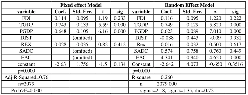
Th results in Table 4, provides both fixed effect model and Random effect model results. Notice that in the fixed effect model R-squared is very high (76%) because the model included dummies for the countries suggesting that country specific effect explain a lot of variation in Tanzanian exports than other postulated factors. An attempt to include time variation (dummies for the years) yielded no
significant improvement in the R-squared suggesting that time variation has little contribution in the variation of Tanzanian exports.
In the fixed effect model time invariant variables were removed from the model and only time variant variables appear as shown. The results in the random effect model indicate distance and SADC dummies to be insignificant. Again, this is due to multicollinearity. When a dummy for EAC was removed both distance and SADC dummies became significant.
Table 4: Fixed Effect Model and Random Effect Model
Fixed effect Model Random Effect Model
variable Coef. Std. Err. t sig variable Coef. Std. Err. z sig
FDI 0.114 0.095 1.19 0.233 FDI 0.116 0.095 1.220 0.222
TGDP 0.743 0.133 5.59 0.000 TGDP 0.749 0.129 5.820 0.000
PGDP 0.648 0.105 6.16 0.000 PGDP 0.623 0.089 7.010 0.000
DIST (omitted) DIST -0.038 0.443 -0.09 0.931
REX 0.028 0.035 0.82 0.412 Rex 0.016 0.032 0.500 0.617
SADC (omitted) SADC 0.574 0.758 0.760 0.449
EAC (omitted) EAC 4.341 0.940 4.620 0.000
constant -2.63 1.756 -1.5 0.134 Constant -2.642 4.073 -0.650 0.3516
p=0.000 p=0.000
Adj-R-Squared=0.76 R-square 0.260
n=2079 n 2079.000
Prob>F=0.000 sigma=2.18, sigma=1.35, rho=0.72
In order to choose the consistent model a hausman test was computed to decide which model to choose. The test shows that the null hypothesis of no systematic difference in coefficients between the two models is not rejected (p=0.84) implying that either of the model can be used for inference. The study opted for a random effect model which is more efficient than a fixed effect model.
The random effect model indicates that Tanzanian GDP, Partner country GDP as well being in East African Community are all significant with positive influence on the Tanzanian exports. The significance of East African Economic Integration provides an evidence for a role of country specific characteristic in influencing exports. This result could have not been obtained in a time series analysis. Unfortunately, time series studies have dominated studies pertaining to Tanzania International trade, including export performance. These results suggest the need for the
government of Tanzania to increase its strategic participation not only to East Africa regional block but as well as to other regional blocks. The results for Tanzanian GDP and Partner country GDP per capita even though significant may not be discussed at this stage much as the two variables are included in a dynamic panel model. Apparently, they show their effects in the absence of lagged exports.
.4.2.3 Dynamic Panel Results to Assess a Country’s Loyalty to its Trading Partners
A GMM estimates as discussed in section 3.2 was estimated in STATA 13 and the results are given in Table 5. The Sargan test for the exogeneity of the used instruments and the test for absence of second order serial correlation are also provided.
Table 5: Dynamic Panel Regression on the Log of Tanzanian Exports
differenced variables Coef. Std. Err. z sig
lnEXit-1 0.173 0.032 5.480 0.000
lnFDIt 0.171 0.082 2.080 0.038
lnTGDPt 0.390 0.159 2.460 0.014
lnPGDPit 0.737 0.194 3.800 0.000
lnREXit 0.038 0.079 0.480 0.633
constant -4.688 1.852 -2.530 0.011 p=0.000
n=1881 sargan test: P=0.85
2nd order serial Correlation test: p=0.56
The results in Table 5 indicates that GMM estimates is significant and that the null hypotheses of instruments exogeneity (sargan test) and of absence of second order serial correlation are both not rejected providing confidence
for the GMM estimates.
matters for Tanzanian exports. An increase in 1% of the current level of exports would lead to an increase in 17 % of the coming exports indicating the importance for a country to handle her customers with a great care.
The results in Table 5 indicate that Tanzanian GDP has a positive and significant influence on Tanzanian exports which is consistent with some time series studies done in Tanzania such as Manamba (2016) and Rwenyagila (2013). The results in Table 5, indicate that an increase in 1% of the Tanzanian GDP would yield an increase of 4% in the country’ exports to the oversee. The message here is very clear that to improve export performance efforts should be made to boost the GDP. The traditional exports account a significant portion of the country exports, implying that boosting agriculture sector could be one of the possible ways to improve the GDP and eventually the export sector. The results in Table 5 also indicates that an increase in 1% of a trading partner GDP per capita would lead to an increase of 7% in the country’s exports. Unfortunately, there is nothing much that the country can do to affect a trading partner income. The best that the country could do is to maintain its trading partners by ensuring efficiency in the services delivery including all export procedures such as the banking processing and the custom department handling procedures as these may influence the country’s loyalty to its trading partners.
Foreign direct investment indicates that an increase in 1% of FDI would lead to an increase in 17% of Tanzanian exports to the oversee. FDI plays a positive role in increasing country’ production capacity which ultimately leads to an increase in exports given other factors equal. The Tanzanian government should keep on attracting FDI’s as one of the possible strategies to boost exports.
5. Conclusion and Recommendations
The study examined determinants of Tanzanian exports under both static and dynamic environment using panel data regression model. It has been found that countries East African Community stands a high chance of consuming Tanzanian products than in other regions. No evidence has been established for countries in the SADC region, even though South Africa is one among the leading importers from Tanzania. Other factors influencing positively Tanzanian exports are the level of past year exports, foreign direct investment. Tanzanian GDP and the trading partner GDP per capita. The study recommends to the government of Tanzania and to other stake holders to actively promote foreign direct investments, to handle the oversee customers with a great care, promoting exports to the oversee through its organs such as TANTRADE, and improving the Tanzanian GDP through rapid industrialization and agriculture improvement.
References
1. Abolagba et al. (2010). Determinants of agricultural exports. Journal of Human Ecology, 29(3): 181-184. 2. Agasha, N. (2007). Determinants of Export Growth
Rate in Uganda 1987-2006.. Uganda Revenue
Authority, Kampala, Uganda.
3. Appleyard et al. (2010). International E conomics. 4. Babatunde. (2009). Can Trade Libralization Stimulate
Export perfomance im Sub-saharan Africa? Journal of
International & Global Economic Studies June 2009.
5. Basu et al. (2000). Promoting growth in sub-Saharan Africa. Learning what works”. Economic Issues
No.23. Washington, DC: IMF.
6. Cameron, A.C and Trivedi, P.K. (2005), Micro econometrics methods and
7. Applications, New York, Cambridge University press, 40 West 20 th Street, NY 10011-4211, USA
8. Chemeda, F. (2001). The Role of Exports in Economic Growth with Reference to Ethiopian country. A paper prepared for the conference on annual meeting of the
agricultural economics association in Chicago.
9. Dijk, M. v. (2002). The Determinants of Export Performance in Developing Countries. Eindhoven Centre for Innovation Studies, The Netherland
Working Paper 02.01.
10. Fosu, A. F. (1990). Export composition and the impact of exports on economic growth of developing countries. Economic Letters 34, pp67-71.
11. Gbetnkom and Khan. (2002). Determinants of agricultural Export. The case of Cameroon, AERC Research Paper 120 African Economic Research
Consortium, Nairobi.