ISSN (Online): 2320-9364, ISSN (Print): 2320-9356
www.ijres.org Volume 2 Issue 6 ǁ June. 2014 ǁ PP.70-87
Estimation Of Optimum Dilution In The GMAW Process Using
Integrated ANN-SA
P Sreeraj
A, T Kannan
b, Subhasismaji
ca
Department of Mechanical Engineering, Valia Koonambaikulathamma College of Engineering and Technology, Kerala, 692574 India.
bPrincipal, SVS College of Engineering,Coimbatore,Tamilnadu,642109 India. cProfessor, Department of Mechanical Engineering IGNOU, Delhi,110068, India.
Abstract
To improve the corrosion resistant properties of carbon steel usually cladding process is used. It is a process of depositing a thick layer of corrosion resistant material over carbon steel plate. Most of the engineering applications require high strength and corrosion resistant materials for long term reliability and performance. By cladding these properties can be achieved with minimum cost. The main problem faced on cladding is the selection of optimum combinations of process parameters for achieving quality clad and hence good clad bead geometry.
This paper highlights an experimental study to optimize various input process parameters (welding current, welding speed, gun angle, contact tip to work distance and pinch) to get optimum dilution in stainless steel cladding of low carbon structural steel plates using Gas Metal Arc Welding (GMAW). Experiments were conducted based on central composite rotatable design with full replication technique and mathematical models were developed using multiple regression method. The developed models have been checked for adequacy and significance. In this study, Artificial Neural Network (ANN) and Simulated Annealing Algorithm (SA) techniques were integrated labels as integrated ANN-SA to estimate optimal process parameters in GMAW to get optimum dilution.
Key words
: Mathematical model, cladding, GMAW, ANN, Clad bead geometry, corrosion, SA.I.
Introduction
Prevention of corrosion is a major problem in Industries. Even though it cannot be eliminated completely it can be reduced to some extent. A corrosion resistant protective layer is made over the less corrosion resistant substrate by a process called cladding. This technique is used to improve life of engineering components but also reduce their cost. This process is mainly now used in industries such as chemical, textiles, nuclear, steam power plants, food processing and petro chemical industries [1].
Most accepted method of employed in weld cladding is GMAW. It has got the following advantages [2]. High reliability
All position capability Ease to use
Low cost
High Productivity
Suitable for both ferrous and non ferrous metals High deposition rate
Cleanliness and ease of mechanization
The mechanical strength of clad metal is highly influenced by the composition of metal but also by clad bead shape. This is an indication of bead geometry. Fig 1 shows the clad bead geometry. It mainly depends on welding current; welding speed, arc voltage etc. Therefore it is necessary to study the relationship between the process parameters and bead parameters to study clad bead geometry. Using mathematical models it can be achieved. This paper highlights the study carried out to develop mathematical and ANN-SA models to optimize clad bead geometry, in stainless steel cladding deposited by GMAW. The experiments were conducted based on four factor five level central composite rotatable designs with full replication technique [3]. The developed models have been checked for their adequacy and significance. Again using ANN-SA, the bead parameters were optimized to get optimum dilution.
network, genetic algorithm fuzzy logic and simulated annealing algorithm. The abilities of ANN include that ANN can handle a nonlinear form of modelling that learns the mapping of inputs to outputs, in terms of speed, simplicity ANN is more successful, ANN models does not need any preliminary assumptions as to underlying mechanisms in the modelled process and there exists ANN tool box in MATLAB which makes the process simple.
Generally modelling is a process of establishing the minimum potential value of welding process while optimization is the process of establishing the potential minimum value of welding performance at optimal point of process parameters. There are some established techniques such as Genetic algorithm (GA), simulated annealing algorithm (SA).Tabu search (TS), and particle swarm optimization technique (PSO).One of the alternative in optimizing weld bead geometry is the use of Simulated annealing algorithm(SA).It is because SA program is easy and typically takes only few hundred lines of computer code, SA algorithm can be used to determine the global minimum more efficiently instead of tapping in a local minimum where objective function has surrounding boundaries and Sa search is independent of initial conditions. The integration system is a combination of two or more techniques with the target to obtain a more successful result.ANN technique and PSO optimization techniques were integrated in determining the optimum solution in conventional machining for pocket –milling and ball end milling process (EI-Mounayri, Kishawy&briceno2005).
In this study an integration system is taken up to observe the possible improvement in the result that may be obtained particularly for GMAW process. With integrated ANN-SA it is expected that it can produce more significant result for dilution compared to the experimental, regression modelling and ANN single based modelling results.
Percentage dilution (D) = [B/ (A+B)] X 100 Fig 1. Clad bead geometry
II.
Experimental Procedure
The following machines and consumables were used for the purpose of conducting experiment.
1) A constant current gas metal arc welding machine (Invrtee V 350 – PRO advanced processor with 5 – 425 amps output range)
2) Welding manipulator 3) Wire feeder (LF – 74 Model)
4) Filler material Stainless Steel wire of 1.2mm diameter (ER – 308 L). 5) Gas cylinder containing a mixture of 98% argon and 2% oxygen. 6) Mild steel plate (grade IS – 2062)
Test plates of size 300 x 200 x 20mm were cut from mild steel plate of grade IS – 2062 and one of the surfaces is cleaned to remove oxide and dirt before cladding. ER-308 L stainless steel wire of 1.2mm diameter was used for depositing the clad beads through the feeder. Argon gas at a constant flow rate of 16 litres per minute was used for shielding. The properties of base metal and filler wire are shown in Table 1.
Estimation of optimum dilution in the GMAW process using integrated ANN-SA
Table 1. Chemical Composition of Base Metal and Filler Wire
III.
Plan of Investigation
The research work was planned to be carried out in the following steps [5]. 1) Identification of factors and responses.
2) Finding limits of process variables. 3) Development of design matrix.
4) Conducting experiments as per design matrix. 5) Recording the responses.
6) Development of mathematical models. 7) Checking the adequacy of developed models. 8) Conducting conformity tests.
3.1 Identification of factors and responses
The following independently controllable process parameters were found to be affecting output parameters. These are wire feed rate (W), welding speed (S), welding gun angle (T), contact tip to work to distance (N) and pinch (Ac), The responses chosen were clad bead width (W), height of reinforcement (R), Depth of Penetration. (P) and percentage of dilution (D). The responses were chosen based on the impact of parameters on final composite model.
The basic difference between welding and cladding is the percentage of dilution. The properties of the cladding are significantly influenced by dilution obtained. Hence control of dilution is important in cladding where a low dilution is highly desirable. When dilution is quite low, the final deposit composition will be closer to that of filler material and hence corrosion resistant properties of cladding will be greatly improved. The chosen factors have been selected on the basis to get minimal dilution and optimal clad bead geometry.
Few significant research works have been conducted in these areas using these process parameters and so these parameters were used for experimental study.
3.2 Finding the limits of process variables
Working ranges of all selected factors are fixed by conducting trial runs. This was carried out by varying one of factors while keeping the rest of them as constant values. Working range of each process parameters was decided upon by inspecting the bead for smooth appearance without any visible defects. The upper limit of given factor was coded as -2. The coded value of intermediate values were calculated using the equation (2)
𝑋𝑖 =
2[2𝑋−(𝑋max +𝑋min )]
(𝑋max − 𝑋min )] --- (2)
Where Xi is the required coded value of parameter X is any value of parameter from Xmin – Xmax. Xmin is the
lower limit of parameters and Xmax is the upper limit parameters [4].
The chosen level of the parameters with their units and notation are given in Table 2.
Table 2. Welding Parameters and their Levels
Parameters Unit Notation Factor Levels
-2 -1 0 1 2
Welding Current A 1 200 225 250 275 300
Welding Speed mm/min S 150 158 166 174 182
Contact tip to work distance mm N 10 14 18 22 26
Welding gun Angle Degree T 70 80 90 100 110
Pinch - Ac -10 -5 0 5 10
Elements wt %
Materials C SI Mn P S Al Cr Mo Ni
IS 2062 0.150 0.160 0.870 0.015 0.016 0.031 - - -
3.3 Development of design matrix
Design matrix chosen to conduct the experiments was central composite rotatable design. The design matrix comprises of full replication of 25(= 32), Factorial designs. All welding parameters in the intermediate levels (o) Constitute the central points and combination of each welding parameters at either is highest value (+2) or lowest (-2) with other parameters of intermediate levels (0) constitute star points. 32 experimental trails were conducted that make the estimation of linear quadratic and two way interactive effects of process parameters on clad geometry [5].
Table 3. Design Matrix
Trial Number Design Matrix
I S N T Ac
1 -1 -1 -1 -1 1
2 1 -1 -1 -1 -1
3 -1 1 -1 -1 -1
4 1 1 -1 -1 1
5 -1 -1 1 -1 -1
6 1 -1 1 -1 1
7 -1 1 1 -1 1
8 1 1 1 -1 -1
9 -1 -1 -1 1 -1
10 1 -1 -1 1 1
11 -1 1 -1 1 1
12 1 1 -1 1 -1
13 -1 -1 1 1 1
14 1 -1 1 1 -1
15 -1 1 1 1 -1
16 1 1 1 1 1
17 -2 0 0 0 0
18 2 0 0 0 0
19 0 -2 0 0 0
20 0 2 0 0 0
21 0 0 -2 0 0
22 0 0 2 0 0
23 0 0 0 -2 0
24 0 0 0 2 0
25 0 0 0 0 -2
26 0 0 0 0 2
27 0 0 0 0 0
28 0 0 0 0 0
29 0 0 0 0 0
30 0 0 0 0 0
31 0 0 0 0 0
32 0 0 0 0 0
Estimation of optimum dilution in the GMAW process using integrated ANN-SA
3.4 Conducting experiments as per design matrix
The experiments were conducted at SVS College of Engineering, Coimbatore, India. In this work thirty two experimental run were allowed for the estimation of linear quadratic and two-way interactive effects of corresponding each treatment combination of parameters on bead geometry as shown Table 3 at random. At each run settings for all parameters were disturbed and reset for next deposit. This is very essential to introduce variability caused by errors in experimental set up.
3.5 Recording of Responses
In order to measure clad bead geometry of transverse section of each weld overlays were cut using band saw from mid length. Position of the weld and end faces were machined and grinded. The specimen and faces were polished and etched using a 5% nital solution to display bead dimensions. The clad bead profiles were traced using a reflective type optical profile projector at a magnification of X10, in M/s Roots Industries Ltd. Coimbatore. Then the bead dimension such as depth of penetration height of reinforcement and clad bead width were measured [6]. The traced bead profiles were scanned in order to find various clad parameters and the percentage of dilution with help of AUTO CAD software. This is shown in Fig 4.
Fig. 4 Traced Profiles (Specimen No.2)
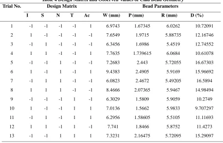
02A represents profile of the specimen (front side) and 02B represents profile of the specimen (rear side). The measured clad bead dimension and percentage of dilution is shown in Table 4.
Table 4 Design Matrix and Observed Values of Clad Bead Geometry
Trial No. Design Matrix Bead Parameters
I S N T Ac W (mm) P (mm) R (mm) D (%)
1 -1 -1 -1 -1 1 6.9743 1.67345 6.0262 10.72091
2 1 -1 -1 -1 -1 7.6549 1.9715 5.88735 12.16746
3 -1 1 -1 -1 -1 6.3456 1.6986 5.4519 12.74552
4 1 1 -1 -1 1 7.7635 1.739615 6.0684 10.61078
5 -1 -1 1 -1 -1 7.2683 2.443 5.72055 16.67303
6 1 -1 1 -1 1 9.4383 2.4905 5.9169 15.96692
7 -1 1 1 -1 -1 6.0823 2.4672 5.49205 16.5894
8 1 1 1 -1 -1 8.4666 2.07365 5.9467 14.98494
9 -1 -1 -1 1 -1 6.3029 1.5809 5.9059 10.2749
10 1 -1 -1 1 1 7.0136 1.5662 5.9833 9.707297
11 -1 1 -1 1 1 6.2956 1.58605 5.5105 11.11693
12 1 1 -1 1 -1 7.741 1.8466 5.8752 11.4273
13 -1 -1 1 1 1 7.3231 2.16475 5.72095 15.29097
02A
W - Width; P - Penetration; R - Reinforcement; D - Dilution %
3.6 Development of Mathematical Models
The response function representing any of the clad bead geometry can be expressed as [7, 8, 9],
Y = f (A, B, C, D, E) --- (3)
Where, Y = Response variable A = Welding current (I) in amps B = Welding speed (S) in mm/min
C = Contact tip to Work distance (N) in mm D = Welding gun angle (T) in degrees E = Pinch (Ac)
The second order surface response model equation can be expressed as below
Y = β0 + β1 A + β2 B + β3 C + β4 D + β5 E + β11 A2 + β22 B2 + β33 C2 + β44 D2 + β55 E2 + β12 AB + β13 AC + β14
AD + β15 AE + β23 BC + β24 BD + β25 BE + β34 CD + β35 CE+ β45 DE --- (4)
Where, β0 is the free term of the regression equation, the coefficient β1,β2,β3,β4 and β5 is are linear terms, the
coefficients β11,β22, β33,β44 and ß55 quadratic terms, and the coefficients β 12,β13,β14,β15 , etc are the interaction
terms. The coefficients were calculated by using MINITTAB 15. After determining the coefficients, the mathematical models were developed. The developed mathematical models are given as follows.
Clad Bead Width (W), mm = 8.923 + 0.701A +0.388B + 0.587C + 0.040D + 0.088E – 0.423A2 – 0.291B2 – 0.338C2 – 0.219D2 – 0.171E2 + 0.205AB + 0.405AC + 0.105AD + 0.070AE – 0.134BC + 0.225BD + 0.098BE + 0.26 CD + 0.086 CE + 0.012 DE --- (5)
14 1 -1 1 1 -1 9.6171 2.69495 6.37445 18.54077
15 -1 1 1 1 -1 6.6335 2.3089 5.554 17.23138
16 1 1 1 1 1 10.514 2.7298 5.4645 20.8755
17 -2 0 0 0 0 6.5557 1.99045 5.80585 13.65762
18 2 0 0 0 0 7.4772 2.5737 6.65505 15.74121
19 0 -2 0 0 0 7.5886 2.50455 6.4069 15.77816
20 0 2 0 0 0 7.5014 2.1842 5.6782 16.82349
21 0 0 -2 0 0 6.1421 1.3752 6.0976 8.941799
22 0 0 2 0 0 8.5647 3.18536 5.63655 22.94721
23 0 0 0 -2 0 7.9575 2.2018 5.8281 15.74941
24 0 0 0 2 0 7.7085 1.85885 6.07515 13.27285
25 0 0 0 0 -2 7.8365 2.3577 5.74915 16.63287
26 0 0 0 0 2 8.2082 2.3658 5.99005 16.38043
27 0 0 0 0 0 7.9371 2.1362 6.0153 15.18374
28 0 0 0 0 0 8.4371 2.17145 5.69895 14.82758
29 0 0 0 0 0 9.323 3.1425 5.57595 22.8432
30 0 0 0 0 0 9.2205 3.2872 5.61485 23.6334
31 0 0 0 0 0 10.059 2.86605 5.62095 21.55264
Estimation of optimum dilution in the GMAW process using integrated ANN-SA
Depth of Penetration (P), mm = 2.735 + 0.098A – 0.032B + 0.389C – 0.032D – 0.008E – 0.124A2– 0.109B2 – 0.125C2 – 0.187D2 – 0.104E2 – 0.33AB + 0.001 AC + 0.075AD + 0.005 AE – 0.018BC + 0.066BD + 0.087BE + 0.058CD + 0.054CE – 0.036DE --- (6)
Height of Reinforcement (R), mm = 5.752 + 0.160A – 0.151B – 0.060C + 0.016D – 0.002E + 0.084A2 + 0.037B2 – 0.0006C2 + 0.015D2 – 0.006E2 + 0.035AB + 0.018AC – 0.008AD – 0.048AE – 0.024BC – 0.062BD – 0.003BE + 0.012CD – 0.092CE – 0.095DE --- (7)
Percentage Dilution (D), % = 19.705 + 0.325A + 0.347B + 3.141C – 0.039D – 0.153E – 1.324A2 – 0.923B2 – 1.012C2 – 1.371D2 – 0.872E2 – 0.200AB + 0.346 AC + 0.602 AD + 0.203 AE + 0.011BC + 0.465BD + 0.548 BE + 0.715 CD + 0.360CE + 0.137 DE --- (8)
3.7 Checking the adequacy of the developed models
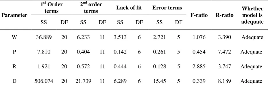
The adequacy of the developed model was tested using the analysis of variance (ANOVA) technique. As per this technique, if the F – ratio values of the developed models do not exceed the standard tabulated values for a desired level of confidence (95%) and the calculated R – ratio values of the developed model exceed the standard values for a desired level of confidence (95%) then the models are said to be adequate within the confidence limit [10]. These conditions were satisfied for the developed models. Values are shown in Table 5.
Table 5 Analysis of variance for Testing Adequacy of the Model
Parameter
1st Order terms
2nd order
terms Lack of fit Error terms
F-ratio R-ratio
Whether model is adequate
SS DF SS DF SS DF SS DF
W 36.889 20 6.233 11 3.513 6 2.721 5 1.076 3.390 Adequate
P 7.810 20 0.404 11 0.142 6 0.261 5 0.454 7.472 Adequate
R 1.921 20 0.572 11 0.444 6 0.128 5 2.885 3.747 Adequate
D 506.074 20 21.739 11 6.289 6 15.45 5 0.339 8.189 Adequate
SS - Sum of squares; DF - Degree of freedom; F Ratio (6, 5, 0.5) = 3.40451; R Ratio (20, 5, 0.05) = 3.20665
IV.
Artificial neural network modelling.
To develop ANN model for predicting the bead geometry a net work structure is illustrated as shown in Fig6.
MAT LAB 7 was used for tracing the network for the prediction of clad bead geometry. Statistical mathematical model was used compare results produced by the work. For normalizing the data, the goal is to examine the statistical distribution of values of each net input and outputs are roughly uniform in addition the value should scaled to match range of input neurons [16].
This is basically range 0 to 1 in practice it is found to between 01 and 9 [17]. In this paper data base are normalized using the Equation (9)
--- (9)
Xnorm = Normalized value between 0 and 1
X = Value to be normalized
Xmin = Minimum value in the data set range the particular data set rage which is to be normalized.
Xmax= Maximum value in the particular data set range which is to be normalized.
In this study five welding process parameters were employed as input to the network. The Levenberg-Marquardt approximation algorithm was found to be the best fit for application because it can reduce the MSE to a significantly small value and can provide better accuracy of prediction. So neural network model with feed forward back propagation algorithm and Levenberg-Marqudt approximation algorithm was trained with data collected for the experiment. Error was calculated using the equation (10).
The difficulty using the regression equation is the possibility of over fitting the data. To avoid this, the experimental data is divided in to two sets; one training set and other test data set .The ANN model is created using only training data the other test data is used to check the behavior the ANN model created. All variables are normalized using the equation (9).The data was randomized and portioned in to two one training and other test data.
... (11)
... (12)
Neural Network general form can be defined as a model shown above y representing the output variables and xj the set of inputs, shown in equation [11, 12]. The subscript i represent the hidden units shown in Fig 6 and
θ represents bias and wj represents the weights. The above equation defines the function giving output as a
function of input.
The training process involves the derivation of weights by minimization of the regularized sum of squared error.
The complexity of model is controlled by the number of hidden level values of regularization constants and is associated with each input one for biases and one for all weights connected to output.
4.1 Procedure for prediction
The effectiveness of ANN model is fully depends on the trial and error process. This study considers the factors that could be influencing the effectiveness of the model developed. In the MATLAB 7 tool there are five Influencing factors listed below.
1. Network algorithm. 2. Transfer function. 3. Training function. 4. Learning function. 5. Performance function.
The ANN structure consists of three layers which are input, hidden, output layer. It is known that ANN model is designed on trial and error basis. The trial and error is carried out by adjusting the number of layers and the number of neurons in the hidden structure. Too many neurons in hidden layer results a waste of computer memory and computation time, while too few neurons, may not provide desired data control effect. The process is conducted using 28 randomly selected samples. Seventeen data are used for training and eleven used for test the data. Table 4 shows randomized data with1-11 for test data and 12-28 for training data.
It is suggested that following guide lines should be followed for selecting training and testing of data such as 90%:10%, 85%:15% and 80%:20% with a total of the 100% combined ratio. To fit the randomized sample of 28; preferred ratio selected is 70%:30%.
1. (70/100) × 28 = 19-20 Training samples. 2. (30/100) × 28 = 8-9 data testing samples.
It is necessary to normalize the quantitative variable to some standard range from 0-1. The number of neurons hidden layers should be approximately equal to n/2, n, 2n and 2n+1 where n is the number of input neurons. Many different ANN network algorithms have been proposed by researchers but back propagation (BP) algorithm has found to be the best for prediction .Researchers developed the model by using feed forward BP and radial basis network algorithm and it were found that feed forward BP gives more accurate results. Basically a feed forward network based on BP is a multilayered architecture made up of one or more hidden layers placed between input and output layers, Shown in Fig 6.Transfer function, training function, learning function and performance function used in this study are logsig, traindgm, traingdx and MSE.
4.2 Determination of the best ANN model
Estimation of optimum dilution in the GMAW process using integrated ANN-SA
Table.6. Comparison of actual and predicted values of the clad bead parameters using neural network data (test)
Tria l No.
Actual Bead Parameters Predicted Bead Parameters Error W (mm) P (mm) R (mm) D (%) W (mm) P (mm) R (mm) D (%) W (mm) P (mm) R (mm) D (%) 1 6.974 3 1.673 5 6.026 2 10.72 1 6.194
5 1.85
5.961 1 12.36 7 0.779 8 -0.177 0.065 1 -1.646 2 7.654 9 1.971 5 5.887 3 12.16 7 7.181 5 2.150 7 6.555 3 10.26 8 0.473 4 -0.179
-0.668 1.899
3 6.345 6 1.698 6 5.451 9 12.74 6 7.495 4 1.533 9 5.492 3 9.380
8 -1.15
0.164
7 -0.04
3.365 2 4 7.763 5 1.739 6 6.068 4 10.61 1 6.493
6 1.854
6.557 3 9.479 9 1.269 9 -0.114 -0.489 1.131 1 5 7.268
3 2.443
5.720 6 16.67 3 7.335 4 2.657 6 5.565 7 19.10 4 -0.067 -0.215 0.154 9 -2.431 6 9.438 3 2.490 5 5.916 9 15.96 7 7.606 6 2.104 5 6.434
2 18.49 1.831
7 0.386 -0.517 -2.523 7 6.082 3 2.467
2 5.492
16.58 9 8.041 7 2.172 2 5.512 6 16.87 4
-1.959 0.295 -0.021 -0.285 8 8.466 6 2.073 7 5.946 7 14.98 5 8.323 6 2.234 9 5.903 1 16.97
2 0.143 -0.161 0.043 6 -1.987 9 6.302 9 1.580 9 5.905 9 10.27 5 8.238 1 1.795 5 5.602 2 11.21 9 -1.935 -0.215 0.303 7 -0.944 10 7.013 6 1.566 2 5.983 3 9.707 3 7.589 9 2.457
9 6.542
13.41 5 -0.576 -0.892 -0.559 -3.708 11 6.295
6 1.586
5.510 5 11.11 7 7.731 8 1.764 7 5.867
6 10.71 -1.436
-0.179
-0.357 0.407
Table.7. Comparison of actual and predicted values of the clad bead parameters using neural network data (training)
Tri al NO .
Actual Bead Parameters Predicted Bead Parameters Error
W (mm) P (mm) R (mm) D (%) W (mm) P (mm) R (mm) D (%) W (mm) P (mm) R (mm) D (%)
1 7.741 1.846 6
5.875 2
11.427
3 7.335 2.098
6
6.079 2
10.82
22 0.406 -0.252 -0.204
0.605 1
2 7.323 1 2.164 75 5.720 95 15.290 97 6.821 4 2.061 7 5.694 6 14.93 79 0.501 7 0.103 05 0.026 35 0.353 07
3 9.617 1 2.694 95 6.374 45 18.540 77 9.371 3 2.898 2 6.408 4 17.45 78 0.245 8 0.203 25 -0.033 9 1.082 97
4 6.633 5
2.308
9 5.554
17.231 38 7.430 6 2.292 7 5.623 2 15.79 08 -0.797 1 0.016 2 -0.069 2 1.440 58
5 10.51 4 2.729 8 5.464 5 20.875 5 7.899 1 2.515 4 5.807 8 18.06 64 2.614 9 0.214 4 -0.343 3 2.809 1
6 6.555 7 1.990 45 5.805 85 13.657 62 6.576 1 1.915 8 5.786 7 14.20 39 -0.020 4 0.074 65 0.019 15 -0.546 2
7 7.477 2 2.573 7 6.655 05 15.741
21 7.393 2.719 1 6.711 2 14.75 25 0.084 2 -0.145 4 -0.056 1 0.988 71
8 7.588 6 2.504 55 6.406 9 15.778 16 7.594 3 2.431 7 6.383 4 15.98 81 -0.005 7 0.072 85 0.023 5 -0.209 9
V.
SIMULATED ANNEALING ALGORITHM OPTIMIZATION
Simulated annealing is a random search technique that able to escape local optima using a probability function (Kirkpatrick,Gelatte,&Vecchi 1983).Based on the iterative improvement ,the SA algorithm is A heuristic method with basic idea of generating random displacement from any feasible solution. This process accepts not only the generated solutions which improve the fitness function but also those which do not improve it with probability function; a parameter depending upon the fitness function.
SA is a method for solving unconstrained and bound-constrained optimization problems. It models the physical process of heating a material and then slowly lowering the temperature to decrease the defects, thus minimizing the system energy. At each of iteration of SA algorithm, new points randomly generated the distance of the new point from the current point or the extent of search is based on the probability distribution of the scale proportional to temperature. The algorithm accepted new scale that lowers the objective but also with the probability points that raise the objective. By accepting points that raises the objective, the algorithms avoids being trapped in the in a local minimum and it is able to globally for mean solutions. An annealing temperature is selected to systematically decrease the temperature as algorithm proceeds. As the temperature reduces the algorithm reduces the extent of its search to converge to a minimum. An important part of SA process is how in puts are randomised .The randomized process take place the previous input value and current temperature inputs. A higher temperature will result more randomization a lower temperature will result less randomization.
In this study Simulated Annealing (SA) which utilizes stochastic optimization is used for the optimization of clad bead geometry deposited by GMAW. The main advantage of using this stochastic algorithm is that global optimization point can be reached regardless of the initial starting point. Since the algorithm incorporates. The major advantage of SA is an ability to avoid being trapped at a local optimum point during optimization .The algorithm employs a random search accepting not only the changes that improve the objective function but also the changes that deteriorate it.Fig.7 shows simulated annealing algorithm [11].
VI.
OPTIMIZATION OF CLAD BEAD GEOMETRY USING SA.
The experimental data related to welding current (I), welding speed(S), welding gun angle (T), Contact tip to work distance (N) and pinch (Ac) are used in the experiments conducted.
The aim of the study is to find optimum adjust welding current (I), welding speed (S), welding Gun angle (T), contact tip to work distance (N) and pinch (Ac) in a GMAW cladding process. The optimum parameters are those who deliver response, as close as possible of the cited values shown in Table 8. Table 9 shows the options used for study.
10 6.142 1 1.375 2 6.097 6 8.9417 99 5.658 3 1.44
6.205 4 9.375 3 0.483 8 -0.064 8 -0.107 8 -0.433 5
11 8.564 7 3.185 36 5.636 55 22.947 21 9.972
4 2.962 5.522 7 18.95 66 -1.407 7 0.223 36 0.113 85 3.990 61
12 7.957 5 2.201 8 5.828 1 15.749 41 9.069 3 2.691 9 6.233 7 17.55 48 -1.111 8 -0.490 1 -0.405 6 -1.805 3
13 7.708 5 1.858 85 6.075 15 13.272 85 6.769 9 1.780
7 6.109 12.85 84 0.938 6 0.078 15 -0.033 8 0.414 45
14 7.836 5 2.357 7 5.749 15 16.632 87 8.536 4 2.943 1 6.673 5 15.96 53 -0.699 9 -0.585 4 -0.924 3 0.667 57
15 8.208 2 2.365 8 5.990 05 16.380 43 8.008
3 2.371 6.018 6 16.37 01 0.199 9 -0.005 2 -0.028 5 0.010 33
16 7.937 1 2.136 2 6.015 3 15.183 74 7.944 1 2.119
7 6.01
15.37 35 -0.007 0.016 5 0.005 3 -0.189 7
Estimation of optimum dilution in the GMAW process using integrated ANN-SA
Table 8. SA Search ranges
Parameters Range
Welding current (I) 200 - 300 Amps
Welding Speed (S) 150 - 182mm/min
Contact tip to work distance(N) 10 - 26mm
Welding gun angle(T) 70 - 110deg
Pinch(Ac) -10 - 10
Table 9. Combination of SA Parameters Leading To Optimal Solution Annealing Function Boltzmann Annealing
Re annealing Interval 100
Temperature update Function Exponential Temperature
Initial Temperature 100
Acceptance probability Function SimulatedAnnealing Acceptance
Data Type Double
The objective function selected for optimizing was percentage of dilution. The response variables bead width (W), Penetration (P), reinforcement (R) and Dilution (D) were given as constraint in their equation. The constrained non linear optimisation is mathematically stated as follows
Minimize f(x)
Subject to f (X (1), X (2), X (3), X (4), X (5)) < 0
Simulated Annealing algorithms are nowadays popular tool in optimizing because SA uses only the values of objective function. The aim of the study is to find the optimum adjusts for welding current, welding speed, pinch, welding angle, contact to tip distance. Objective function selected for optimization was percentage of dilution. The process parameters and their notation used in writing the programme in MATLAB 7 software are given below.
Minimize f(x)
Subject to (X (1), X (2), X (3), X (4), X (5)) < 0 X (1) = Welding current (I) in Amps X (2) = Welding Speed (S) in mm/min
X (3) = Contact to work piece distance (N) in mm X (4) = Welding gun angle (T) in degree
X (5) = Pinch (Ac)
Objective function for percentage of dilution which must be minimized was derived from equation 5-8. The constants of welding parameters are given Table 2.
Subjected to bounds 200 ≤ X (1) ≤ 300
150 ≤ X (2) ≤ 182 10 ≤ X (3) ≤ 26 70 ≤ X (4) ≤ 110 -10 ≤ X (5) ≤ 10
6.1 Objective Function
f(x)=19.75+0.325*x(1)+0.347*x(2)+3.141*x(3)-0.039*x(4)-0.153*x(5)-1.324*x(1)^2-0.923*x(2)^2-1.012*x(3)^2-1.371*x(4)^2-0.872*x(5)^20.200*x(1)*x(2)+0.346*x(1)*x(3)+0.602*x(1)*x(4)+
0.203*x(1)*x(5)+0.011*x(2)*x(3)+0.465*x(2)*x(4)+0.548*x(2)*x(5)+0.715*x(3)*x(4)+0.360*x(3)*x(5)+ 0.137*x(4)*x(5) ………..(13)
6.2 Constraint Equations
0.036*x(4)*x(5))-3 ………...………..(15) (Depth of penetration (P) upper limit),
P=(2.735+0.098*x(1)-0.032*x(2)+0.389*x(3)-0.032*x(4)-0.008*x(5)-0.124*x(1)^2-0.109*x(2)^2-
0.125*x(3)^2-0.187*x(4)^2-0.104*x(5)^2-0.33*x(1)*x(2)+0.001*x(1)*x(3)+0.075*x(1)*x(4)+0.005*x(1)*x(5)-0.018*x(2)*x(3)+0.066*x(2)*x(4)+0.087*x(2)*x(5)+0.058*x(3)*x(4)+0.054*x(3)*x(5)-0.036*x(4)*x(5))+2 ………...……..(16)
(Depth of penetration (P) lower limit),
f(x)-23.6334 ………(20)
8.94441799-f(x) ……….……… (21) (Dilution Upper and lower limit),
x(1),x(2),x(3),x(4),x(5) ≤ 2; ...(22) x(1),x(2),x(3),x(4),x(5) ≥ -2; ...(23)
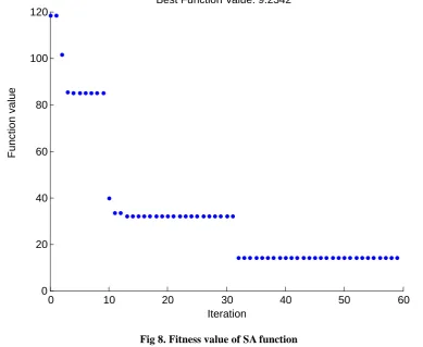
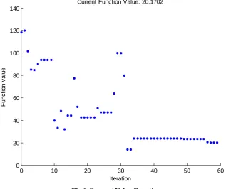
Other constraint equations bead width ,reinforcement are written in same format as penetration for writing the programme. MATLAB program in SA and SA function was used for optimizing the problem. The program was written in SA and constraints bounds were applied. The minimum percentage of dilution obtained from the results obtained running the SA tool. The minimum percentage of dilution obtained is 9.2342.the value of process parameters obtained is I=240amp, S=157mm/min, N=13mm, T=87egrees, Ac=4.5.The fitness function is shown in Fig 8.Fig 9 shows current value function.
Fig 8. Fitness value of SA function
0 10 20 30 40 50 60
0 20 40 60 80 100 120
Iteration
Best Function Value: 9.2342
F
un
c
ti
o
n v
al
Estimation of optimum dilution in the GMAW process using integrated ANN-SA
Fig 9.Current Value Function
VII.
Methodology of integrated ANN-SA
The methodology applied in this study involves six cases [18]. They are experimental data, regression modelling, ANN single based modelling SA single based optimization, integrated ANN-SA–type-A based optimization and integrated ANN-SA–type-B based optimization. The objectives of type-A and type-B are.
1. To estimate the minimum value of cladding parameters compared to the performance value of the experimental data, regression modelling and ANN single based modelling.
2. To estimate the optimal process parameters values that has been within the range of minimum and maximum coded values for process parameters of experimental design that are used for experimental trial.
3. To estimate the optimal solution of the process parameters within the small number of iterations compared to the optimal solution of the process parameters with single based SA optimization.
The steps in order to implement the integrated ANN-GA –type-A and integrated ANN-GA type-B in fulfilling the three objectives are:
1. In the experimental data module the values of dilution for different combinations of process parameters used for modelling.
2. In the regression modelling schedule model was developed using cladding process parameters. A multilinear regression analysis was performed to predict dilution and a governing equation was constructed.
3. A predicted model was developed using ANN. The percentage if error was calculated between predicted and actual values.
4. In the single based SA optimization, the predicted equation of the regression model would become the objective function .The minimum and maximum coded values of the process parameters of the experimental design would define the boundaries for minimum and maximum values of the optimal solution.
5. In the integrated ANN-SA-type-A module that it was the first integration system proposed in this study. Similar to SA single based optimization process the predicted equation of the regression would become the objective function. This integration system process the optimal process parameters value of the single based SA optimization process combined with the process parameters of ANN system would define the foundries if minimum and maximum values for optimal solution.
6. In the integrated ANN-SA-type-B system which is the second integration system proposed in this study. Similar to type A the predicted regression equation would become the objective function and the optimal process parameters value of single based SA optimization combined with process parameters value of the ANN model would define the boundaries for the minimum and maximum values of the optimal solution
0 10 20 30 40 50 60
0 20 40 60 80 100 120 140
Iteration
F
u
n
c
ti
o
n
v
a
lu
e
.This integration system proposes the process parameters values of the best ANN model to define the initial point for optimization solution [19].
7.1 Integrated ANN-SA-type-A optimization solution
The strategy of this study in implementing integrated ANN-GA-type-A is by proposing the optimal process parameters value of the SA combined with the non-optimal process parameters value of the ANN model to define the boundaries for the minimum and maximum value for optimization solution. As given in Table 6, the non-optimal process parameters values that yield to the minimum prediction, value of the ANN model for dilution are D%=9.353, I= 250Amps, S= 166mm/min, N = 10 mm, T = 10degree and Ac=0. As given in Fig. 8, the values of optimal process parameters from SA are I= 240 amps, S= 157mm/min, N = 13 mm. T = 87degrees and Ac = 4.5.
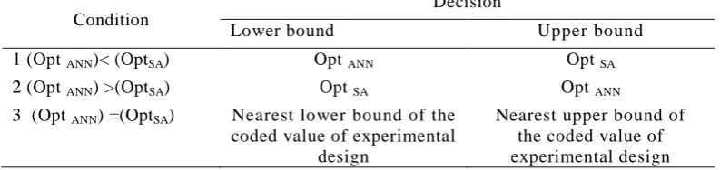
Three conditions could he stated for the non-optimal process parameters values of the ANN model (OptANN) and optimal process parameters values of the SA (OptSA) as classified in Table 10.
By using the conditions stated in Table 12, the decision to define the limitation constraint bound values of the optimization solution are given. Fulfilling the above condition Eqns. (24)- (28) are formulated to define the limitation constraint bounds for welding current, welding speed, contact tip to work distance, welding angle and pinch as process parameters, respectively. The limitation constraint bound for each process parameters are stated as follows [20]:
240 ≤ I≤ 250 (24)
157≤ S≤166 (25)
10≤ N≤ 13 (26)
8 7 ≤ T≤ 9 0 (27)
0≤ Ac≤ 4.5 (28)
As per Fig. 10 the optimal process parameters value that lead to the minimum cladding performance of the S A is proposed to define initial points for the integrated ANN-SA-type-A to search the optimal solution. The equations for the initial point of optimization solution for integrated ANN -SA-type A are given in Eq. (29 ), (30). (31), (32), (33) as follow. Fig 9 shows the values.
Initial point of I = 240 (29) Initial point of S =157 (30) Initial point of N=10 (31) Initial point of T = 87 (32) Initial point of Ac= 0 (33)
Table 12.Condition to define limitation const raint bounds of integrated ANN -SA.
Condition
Decision
Lower bound Upper bound
1 (Opt ANN)< (OptSA) Opt ANN Opt SA
2 (Opt ANN) >(OptSA) Opt SA Opt ANN
3 (Opt ANN) =(OptSA) Nearest lower bound of the
coded value of experimental design
Nearest upper bound of the coded value of experimental design
Estimation of optimum dilution in the GMAW process using integrated ANN-SA
Fig11 . Fitness value of ANN -SA Type -A
It can be seen that the set values of optimal process parameters that lead to the minimum dilution D= 9.1197% are I= 274amps, S=152mm/min, N=12mm, T=73degrees and Ac=1.4.
7.2. Integrated ANN-SA-type-B optimization solution
Similar to integrated ANN-SA-type-A approach, the objective function formulate in Eq. (13), The basic difference to the integrated ANN-SA-type-A approach, the non-optimal process parameters value that lead to the minimum machining performance of the best ANN model that stated shown in Fig. 11 is proposed to define initial point for the integrated
ANN-SA-type-B is to search the optimal solution. Therefore, the equation for the initial point for integrated ANN-SA-type-B could be given in Eq. (32) to (36) as follows:
Initial point of I = 250 (32) Initial point of S =166 (33) Initial point of N =10 (34) Initial point of T =90 (35) Initial point of Ac = 0 (36)
The results of the integrated ANN- SA-type-B by using MATLAB Optimization Toolbox fitness function are as shown in Fig.12.
Fig 13.Current point
From Fig 12, it can be seen that the set values of optimal process parameters that lead to the minimum value of dilution D = 9.0197 are I=212amps=138mm/min, N=16mm, T=78degrees and Ac=1.5. Fig.13 Shows current point.
7.3 ANN-SA Type-A
D=19.75+0.325*x(1)+0.347*x(2)+3.141*x(3)-0.039*x(4)-0.153*x(5)-1.324*x(1)^2-0.923*x(2)^2-
1.012*x(3)^2-1.371*x(4)^2-0.872*x(5)^2-0.200*x(1)*x(2)+0.346*x(1)*x(3)+0.602*x(1)*x(4)+0.203*x(1)*x(5)+0.011*x(2)*x(3)+0.465*x(2)*x(4)+0.548 *x(2)*x(5)+0.715*x(3)*x(4)+0.360*x (3)*x(5) +0.137*x (4)*x (5) ..……… (37)
Optimum dilution obtained is 9.9532 7.4 ANN-SA Type-B
D=19.75+0.325*x(1)+0.347*x(2)+3.141*x(3)-0.039*x(4)-0.153*x(5)-1.324*x(1)^2-0.923*x(2)^2-1.012*x(3)^2-1.371*x(4)^2-0.872*x(5)^2-0.200*x(1)*x(2)+0.346*x(1)*x(3)+0.602*x(1)*x(4)+ 0.203*x(1)*x(5)+ 0.011*x(2)*x(3)+0.465*x(2)*x(4)+0.548*x(2)*x(5)
+0.715*x(3)*x(4)+0.360*x(3)*x(5)+0.137*x(4)*x (5) …..………… (38)
Optimum dilution obtained is 9.7895
VIII.
Validation of the integrated ANN-SA result
Theoretically, to validate the result of the proposed approach this study, the optimal process parameters values of the inte grated ANN -SA will be transferred into the regression model equation. Eq. (13), taken as the objective function of the optimization solution where I an optimal solution of the welding current . S an optimal solution of the welding speed; N is an optimal solution of contact to work distance. T is an optimal solution of the welding gun angle, and Ac an optimal solution of the pinch of integrated ANN-SA, this study discusses the calculation for validating the result of integrated ANN-SA-type-A and integrated ANN-SA-type-B.
IX.
Evaluation of the integrated ANN -SA results
In this study, discussion is carried out to highlight all the objectives of the study is separated into three parts which are evaluation of the minimum Dilution value, evaluation of the optimal process parameters and evaluation of the number of iteration of the integrated ANN-SA results.
9.1. First objective: Evaluation of the minimum Dilution value
Fig. 11 and Fig. 12 show the minimum value of dilution for both integration s ys t e ms , i n t e g r a t e d A N N - S A - t yp e - A a n d A N N - S A - t yp e - B a r e 9 . 0 1 9 7 . For fulfilling the first objective of this study, evaluation against the minimum dilution is 9.237 by SA.
1 2 3 4 5
-1.5 -1 -0.5 0 0.5 1 1.5 2
Current Point
Number of variables (5)
C
u
rr
e
n
t
p
o
in
Estimation of optimum dilution in the GMAW process using integrated ANN-SA
9.2. Experimental data vs. integrated ANN-SA
Optimum dilution should be between 8-15% from previous study .This objective is fulfilled in this case.
9.3. Regression vs. integrated ANN
The minimum predicted dilution value of the regression model is 9.9532. Therefore, with dilution is 9.0192. It can be concluded that both integration systems have given the more minimum result of the dilution compared to regression model. Conseq uently, integrated ANN -SA-type-A and integrated ANN -SA-type-B have reduced the value of dilution and optimized between 8 to15.
9.4. ANN vs. integrated ANN-SA
Minimum predicted Dilution value of the ANN model is9.353, it can he concluded that both integration systems have given the more optimum result of the Dilution compared to ANN model. Consequently, integrated ANN -SA-type-A and integrated ANN -SA-type-Aare well within the limits of standard dilution .
9.5. SA vs. integrated ANN-SA
The minimum predicted Dilution value of the SA was 9.375. Therefore, with Dilution 9.745, it can be concluded that both integrated systems have given the more minimum of the Dilution compared to SA technique.
9.6. Second objective: Evaluation of the optimal process parameters
For the second objective of this study, the optimal values of the integrated ANN-SA-type-A and integrated ANN-SA-type-B for each process parameter are within the range of minimum and maximum value of experimental design, thus, this study concludes that the second objective of this study is fulfilled.
9.7. Third objective: Evaluation of the number of iteration
Integrated ANN-SA-type-A and integrated ANN-SA-type-B are approximately same or lower than the number of iteration by SA, thus, this study concludes that the third objective of this study is fulfilled.
X.
Conclusion
This study proposed two integration systems, integrated ANN -SA-type-A and integrated ANN-SA-type- B, in order to estimate the optimal solutions of process parameters that lead to minimum dilution is found to satisfy three conditions. The process parameters considered for this study are Welding current(I),Welding speed(S),Contact tip to work distance(N),Welding gun angle(T),and pinch(Ac).The outputs are Bead width(W),Penetration(P) ,Height of reinforcement(R) and Dilution(D).Each process parameters recommended by ANN -SA-type-A and integrated ANN-SA-type-B have satisfied within the minimum and maximum range of coded values for process parameters of experimental design. It also showed that number of iterations improved.
References
[1] Palani. P. K, Murugan N. „Prediction of Delta ferrite Content and Effect of Welding Process Parameters in Claddings by FCAW‟
– Journal of Materials and Manufacturing Process (2006) 21:5pp 431-438
[2] Kannan.T and Murugan.N. „Prediction of ferrite number of duplex stainless steel clad metals using RSM‟- Welding Journal
(2006) pp 91-s to 99-s
[3] Gunaraj V. and Murugan N. „ Prediction and control of weld bead geometry and shape relationships in submerged arc welding of
pipes‟- Journal of Material Processing Technology (2005) Vol. 168, pp. 478 – 487.
[4] KimI.S, SonK.J, YangY.S,Yaragada P. K. D.V, „Sensitivity analysis for process parameters in GMA welding process using
factorial design method’- International Journal of Machine tools and Manufacture (2003) Vol. 43, pp. 763 to 769
[5] Cochran W.G and CoxzG.M. Experimental Design(1987) pp.370, New York, John Wiley & Sons
[6] SerdarKaraoglu, Abdullah Secgin „Sensitivity analysis of submerged arc welding process parameters’ – Journal of Material
Processing Technology (2008) Vol-202, pp 500-507
[7] Ghosh P.K, Gupta P.C. and Goyal V.K. „Stainless steel cladding of structural steel plate using the pulsed current GMAW
process‟- Welding Journal (1998) 77(7) pp.307-s-314-s.
[8] Gunaraj V. and Murugan N. „Prediction and comparison of the area of the heat effected zone for the bead on plate and bead on
joint in SAW of pipes’ – Journal of Material processing Technology. (1999) Vol. 95, pp. 246 to 261.
[9] Montgomery DC „Design and analysis of Experiments’ (2003) –John Wiley & Sons (ASIA) Pvt. Ltd.
[10] Kannan T., Yoganath „Effect of process parameters on clad bead geometry and shape relationships of stainless steel cladding
deposited by GMAW’ – Int. Journal of Manufacturing Technology (2010)Vol-47, pp 1083-1095
[11] PraikshitDutta, Dilip Kumar Pratihar „Modelling TIG welding process using conventional regression analysis and neural network
[12] HakanAtes, „Prediction of gas welding parameters based on artificial neural networks’- Materials and Design 2007 (28) 2015 – 2023.
[13] Lee J.I,K.W. Um, „Prediction of welding process parameters by prediction of back bead geometry’-Journal of materials
processing technology 2000 (108,) 106 – 113.
[14] AnanyaMukhopadhyay, AsifIqbal. ‘Prediction of Mechanical Properties of Hot Rolled, Low-Carbon Steel Strips Using Artificial
Neural Network’ – Journal of Material and Manufacturing Process (2007) 20:5, 793-812.
[15] Deepak Kumar Panda, Rajat Kumar Bhoi. „Artificial Neural Network Prediction of Material Removal Rate in Electro Discharge
Machining’ – Journal of Materials and Manufacturing Process (2007) 20:4, 645-672
[16] D. S Nagesh, G. L Datta „Prediction of weld bead geometry and penetration in shielded metal arc welding using artificial neural
network’- Journal of Material Processing Technology (2002) Vol. 123 pp 303-312
[17] N. Manikyakanth, K. SrinivasaRao P. „Prediction of bead geometry in pulsed GMA welding using back propagation neural
network‟ – Journal of Material Processing Technology (2008) Vol-200, pp -300-305
[18] AzlanMohdZain,HabibollahHaron,Safian Sharif “Optimization of process parameters in abrasive water jet machining using
integrated SA-GA” –Applied soft computing(2011),11.5350-5359.
[19] AzlanMohdZain,HabibollahHaron,SafianSharif “Estimation of the minimum machining performance in the abrasive water jet
machining using integrated ANN-SA” Expert systems with applications(2011),38, 8316-8326