Multi-PI Control for Block-structured Nonlinear
Systems
Jingjing Du
State Key Lab. of Industrial Control Technology, Institute of Industrial Process Control, Zhejiang University, Hangzhou 310027, China
School of Electrical Engineering and Automation, Henan Polytechnic University, Jiaozuo 454000, China Email: [email protected]
Chunyue Song
State Key Lab. of Industrial Control Technology, Institute of Industrial Process Control, Zhejiang University, Hangzhou 310027, China
Email: [email protected]
Abstract—A Multi-PI control strategy is presented for block-structured nonlinear systems, aiming to overcome the drawbacks of the conventional nonlinearity inversion control method and improve the closed-loop control performance. Besides, the proposed Multi-PI method applies the traditional PI control algorithm to complex nonlinear systems, simplifying the control problems largely and reducing computation load greatly. Two benchmark systems are studied to demonstrate the effectiveness of the proposed control method.
Index Terms—block-structured systems, Multi-PI control, included angle dividing method, nonlinearity inversion method
I. INTRODUCTION
Block-structured nonlinear systems mainly denote systems with a Hammerstein or a Wiener model structure. They consist of the cascade connection of a linear dynamic block and a nonlinear static block [1, 2], which makes the system analysis and control design easy. Hammerstein and Wiener model structures have proved to be effective in representing and approximating many industrial processes, as they may account for nonlinear effects encountered in most chemical processes [3], such as pH neutralization processes, distillation columns, heat exchangers, polymerization reactor, dryer process and so on [3, 4].
When a block-structured model is used for control purposes, the conventional control strategy is the nonlinearity inversion method [2, 5, 6], which makes full
use of advantages of the block structure, and is easy and effective in most cases. However, this method needs the static nonlinear element to be bijective, which is generally not the case [5], especially when the nonlinearity systems exhibit input or output multiplicity. Besides, nonlinearity inversion may lead to performance degradation [7]. So many other methods have been tried to overcome these disadvantages. In Ref. [7], the static input nonlinearity is transformed into a polytopic description, and then a linear MPC constrained to LMIs is designed. Whereas, the method also needs the nonlinear element to be invertible. In Ref. [5], a NMPC based on sensitivity analysis is proposed for block-structured system. However, the sensitivity calculation involves solution of a series of partial differential equations, which makes the whole method complicated.
In this article, a Multi-PI control method is proposed for block-structured systems aiming to overcome the shortcomings of the conventional nonlinearity inversion method and solve the troublesome control problem of non-invertible block-structured systems in a classic and simple way. In the proposed method, a complex nonlinear control problem is decomposed into a set of simple linear control problems, which largely reduces the complexity and computation burden, solves the control of systems with input/output multiplicity in an easy way, and further avoids the performance degradation involving with the common nonlinearity inversion method. Two chemical processes are studied to illustrate the effectiveness of the proposed Multi-PI control method for block-structured systems with strong nonlinearity.
II. BLOCK-STRUCTURED SYSTEMS
A. Block-Structrued Systems
Hammerstein models and Wiener models are popular nonlinear empirical modeling structures [1], and have been applied to many chemical processes [3], such as pH neutralization processes, distillation columns, heat
Manuscript received November 1, 2011; revised November 10, 2011; accepted November 12, 2011.
This work is supported partially by the NSF (60974023, 61104079) of China, partially by the Fundamental Research Funds for the Central Universities, and partially by the Doctors’ Funds (B2011-007) of Henan Polytechnic University.
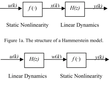
exchangers, polymerization reactor and so on. As is depicted in Fig. 1, a Hammerstein model is a block-structured nonlinear model, which consists of the cascade structure of a static nonlinear function f (·) followed by a linear dynamic block H(z), whereas a Wiener model contains the same elements in the reverse order [1]. Thanks to their special structure, there is an excellent property for them. That is their nonlinear characteristic lie in the static gains not in the dynamics [8]. This property makes it convenient to get an effective model for complex systems, and facilitates the corresponding system analysis and controller design.
Figure 1a. The structure of a Hammerstein model.
Figure 1b. The structure of a Wiener model.
The Hammerstein model and Wiener model are described by Eq. (1) and Eq. (2), respectively.
1 1
( ) ( ( ))
( ) ( ) ( )
n m
i i
i i
x k f u k
y k a y k i b x k i
= =
= ⎧ ⎪
⎨ = − + −
⎪⎩
∑
∑
(1)
1 1
( ) ( ) ( )
( ) ( ( ))
n m
i i
i i
w k a w k i b u k i
y k f w k
= =
⎧ = − + −
⎪ ⎨
⎪ =
⎩
∑
∑
(2)where, x and w are intermediate variables; and f (·) is analytic and not necessarily invertible in this work.
Hammerstein and Wiener model structures have been popular in modeling industrial processes, as they are able to capture the nonlinear effects encountered in most chemical processes [3]. Chemical processes such as pH neutralization processes, distillation columns, heat exchangers, polymerization reactor, dryer processes, and so on, have been modeled by block-structured models [4]. In this work, two benchmark block-structured systems are studied. One is a Hammerstein system-a Heat Exchanger process, and another is a Wiener system-a pH process. B. Nonlinearity Inversion Method
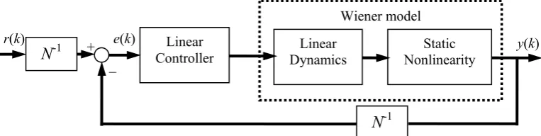
Block-structured models are popular for their special structure that facilitates the analysis of nonlinear processes and has an underlying potential for controller design. A popular control approach for block-structured models is the nonlinearity inversion method [2, 5, 6], which consists of the follows steps:
Firstly, remove the static nonlinearity from the original control problem via the inversion of the nonlinear element N-1(·) and convert the nonlinear control problem
into a new linear one, i.e., design a linear controller based on the linear dynamic element H(z).
Secondly, convert the linear controller into a nonlinear one by the nonlinear inversion N-1(·).
Thirdly, implement the output of the nonlinear controller on the block-structured system.
The conventional nonlinearity inversion control strategy for Hammerstein and Wiener models is shown in Fig. 2a and Fig. 2b.
From the procedure above, we can see that the key to the nonlinearity inversion method is the invertibility of the nonlinear element N(·). However, the invertibility condition is not always satisfied [5, 9]. For example, when a Hammerstein system exhibits input multiplicity, or a Wiener system has output multiplicity, which can arise in practical processes, the static nonlinearity N(·) is not invertible. Under such circumstances, the nonlinearity inversion method fails. Thus, other control approach must be exploited to deal with non-invertibility cases.
III. MULTI-PI CONTROL OF BLOCK-STRUCTURED SYSTEMS
A. Multi-model Representation of Block-Structrued Nonlinear Systems
The multi-model control approach has proved to be useful in dealing with nonlinear control problems, and has attracted much attention and been studied extensively in the past years [10-16]. The major motivation for the multi-model control approach is that local linear modeling is simpler than global modeling because locally there are less relevant phenomena and simpler interactions [16], and that the classic control techniques can be used to simplify the nonlinear control problems. The basic concept of multi-model control is to represent a complex nonlinear system as a combination of linear systems to which classical control techniques can be easily applied [13]. Obviously, it is applicable to block-structured systems and may have potential advantages over the nonlinearity inversion method and other control methods.
Recently, an included angle based nonlinearity measure was proposed to assess the nonlinearity degree of SISO block-structured systems [17]. The absolute difference between the slope angles of two operating points along the static input-output curve is defined as the included angle of the two operating points. And further, the biggest included angle over an operating space is defined as the nonlinearity measure for the system in this operating space. Based on the included angle based nonlinearity measure, an included dividing method is proposed for SISO block-structured systems [15], which can effectively divide a block-structured nonlinear system into a set of well-approximating linear submodels. The key point of the dividing method is to divide a block-structured nonlinear system into a set of linear models according to the slope variation of its static I/O curve. Then a global multi-model controller can be designed to avoid the shortcomings in the common nonlinearity inversion method. In this section, we analyze the multi-
u(k) f (·) x(k) H(z) y(k)
Static Nonlinearity Linear Dynamics
u(k) H(z) w(k) f (·) y(k)
model representation of block-structured nonlinear systems.
For the Hammerstein model (1), it can be rewritten as the following NARMAX form [1, 15,18-20].
1 2
1 2
( )
( ( ))
(3)
( )
( 1)
( 2) ...
(
)
( 1)
( 2) ...
(
)
(4)
n m
x k
f u k
y k a y k
a y k
a y k n
bx k
b x k
b x k m
=
⎧
⎪
=
− +
− + +
−
⎨
⎪ +
− +
− + +
−
⎩
where, f (·) is analytic and not necessarily invertible. The intermediate variable x can be removed from Eq. (3)-(4). Substitute Eq. (3) into Eq. (4), we get the following NARMAX equation.
1 2
1 2
( ) ( 1) ( 2) ... ( )
( ( 1)) ( ( 2)) ... ( ( ))
n m
y k a y k a y k a y k n
b f u k b f u k b f u k m
= − + − + + −
+ − + − + + − (5)
Let ΩH be the full operating space of Hammerstein
system (5) and apply the included angle dividing method [15] to it step by step. First choose a threshold value and the number of steady-state points to grid ΩH according to
a priori knowledge. Then calculate the included angle matrix of the steady-state points. Finally, divide the operating space ΩH using the included angle matrix
according to the algorithm in Ref. [15]. Suppose the operating space ΩH of the Hammerstein system (5) is
decomposed into m subspaces ΩHi, i = 1, 2, …, m. Each
subspace has an operating point (u0i, y0i) in it. At the
operating point we have
1
1 0 2 0 0
1 0 2 0
0
( ) ( 1) ... ( )
( ( 1)) ( ( 2)) ... ( ( ))
'( ( 1)) ( 1) '( ( 2)) ( 2) ...
'( ( )) ( )
n
i i m i
i i
m i
y k a y k a y k n
b f u k b f u k b f u k m
b f u k u k b f u k u k
b f u k m u k m
− − − − −
= − + − + + −
+ − Δ − + − Δ − +
+ − Δ −
(6)
At operating point (u0i, y0i), the following three
equations exist.
0 0 0
0 0 0
0 1 0 0
1 0 0
( ) ( 1) ... ( ),
( ) ( 1) ... ( ),
( ) ( 1) ... ( ) ...
( ( 1)) ... ( ( ))
i i i
i i i
i i n i
i m i
y k y k y k n
u k u k u k m
y k a y k a y k n
b f u k b f u k m
= − = = −
= − = = −
= − + − +
+ − + + −
(7)
Substitute Eq. (7) into Eq. (6), we get:
1
1 0
0
( ) ( 1) ... ( )
'( ( 1)) ( 1) ...
'( ( )) ( )
n i
m i
y k a y k a y k n
b f u k u k
b f u k m u k m
Δ − Δ − − − Δ −
= − Δ − +
+ − Δ −
(8)
So we obtain the transfer function of Eq.(8) as follows:
1 1
0 1
1 ...
( ) '( ( ))
1 ...
m m
Hi n i
n
b z b z
G z f u k
a z a z
− −
− −
+ + =
− − − ,
i=1, 2, …, m. (9) Eq. (9) is the linearized model of Hammerstein system (1) around operating point (u0i, y0i). For m subspaces,
there are m linearized models. So Eq. (9) can also be considered as the multi-model representation of the Hammerstein system (1). Besides, from Eq. (9), it is seen that the zeros and poles of the Hammerstein model Eqs. (3)-(4) is constant, and they do not vary as operating point changes, while the steady-state gain varies with operating point. It confirms the conclusion that the nonlinear characteristic of Hammerstein system is primarily static but not dynamic [8,20-23].
In the same way, we analyze the multi-model description of the Wiener system (2) as follows.
Rewrite the Wiener model (2) as
1 2
1
( ) ( 1) ( 2) ...
( ) ( 1) ... ( )
( ) ( ( ))
n m
w k a w k a w k
a w k n bu k b u k m
y k f w k
= − + − +
⎧
⎪ + − + − + + − (10)
⎨
⎪ = (11) ⎩
y(k) Linear
Controller
N
-1 Nonlinearity Static Dynamics Linear Hammerstein model e(k)−
r(k) +
Figure 2a. The nonlinear inversion control strategy for a Hammerstein model
Figure 2b. The nonlinear inversion control strategy for a Wiener model
y(k) Linear
Controller
N
-1 e(k) Dynamics Linear Nonlinearity Static −r(k) +
N
-1For convenience, but without of loss of generality, we suppose f (·) is invertible, and its inverse function is g (·), then we get Eq. (12)
( )
( ( ))
w k
=
g y k
(12) Substitute Eq. (12) into Eq. (10) and remove the intermediate variable w, we get Eq. (13).1 2
1
2
( ( )) ( ( 1)) ( ( 2)) ... ( ( )) ( 1) ( 2) ... ( )
n
m
g y k a g y k a g y k a g y k n b u k
b u k b u k m
= − + − +
+ − + −
+ − + + −
(13)
Suppose the entire operating space of Wiener system (2) to be ΩW which is decomposed into m subspaces ΩWi,
i = 1, 2, …, m according to the included angle dividing method. Linearize Eq. (13) around the operating point (u0i,
y0i) of the ith subspace, we get:
0 1 0
2 0 0
0 1 0
2 0
0
1 2
( ( )) ( ( 1))
( ( 2)) ... ( ( ))
( ( )) ( ) ( ( 1)) ( 1)
( ( 2)) ( 2) ...
( ( )) ( )
( 1) ( 2) ... ( )
n
n
m
g y k a g y k
a g y k a g y k n
g y k y k a g y k y k
a g y k y k
a g y k n y k n
bu k b u k b u k m
− −
− − − − −
′ ′
+ Δ − − Δ −
′
− − Δ − −
′
− − Δ −
= − + − + + −
(14)
At operating point (u0i, y0i), the following three
equations exist.
0 0 0
0 0 0
0 1 0 0
1 0 0
( ) ( 1) ... ( ),
( ) ( 1) ... ( )
( ( )) ( ( 1)) ... ( ( ))
... ( 1) ... ( )
n m
y k y k y k n
u k u k u k m
g y k a g y k a g y k n
bu k b u k m
= − = = −
= − = = −
= − + + −
+ − + + −
(15)
Substitute Eq.(15) into Eq.(14), we get:
0 1 0
2 0
0
1 2
( ( )) ( ) ( ( 1)) ( 1)
( ( 2)) ( 2) ...
( ( )) ( )
( 1) ( 2) ...
( )
n
m
g y k y k a g y k y k
a g y k y k
a g y k n y k n
b u k b u k
b u k m
′ Δ − ′ − Δ −
′
− − Δ − −
′
− − Δ −
= Δ − + Δ − +
+ Δ −
(16)
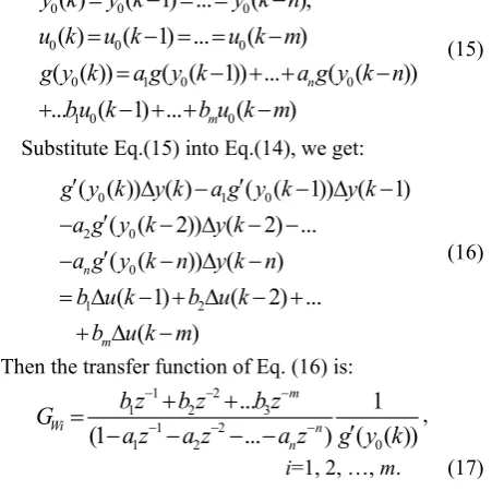
Then the transfer function of Eq. (16) is:
1 2
1 2 3
1 2
1 2 0
... 1
(1 ... ) ( ( ))
m
Wi n
n
b z b z b z
G
a z a z a z g y k
− − −
− − −
+ +
=
′
− − − − ,
i=1, 2, …, m. (17)
Eq. (17) is the multi-model representation of the Wiener system (2). Obviously, for a Wiener model, its nonlinearity also lies in static characteristics but not dynamics.
In summary, block-structured nonlinear systems have primarily static nonlinearity, while their dynamics are basically linear. This is the special property belongs to block-structured nonlinear systems. And the included angle dividing method [16] is based on this property. B. Multi-PI control Algorithm for Block-structured Systems
After the dividing and linearization above, we get a set of linear models Eq. (9) or (17), which can well approximate the block-structured nonlinear system. The control problem of a block-structured nonlinear system is then transformed into controlling a series of linear subsystems, which can be easily and effectively solved by traditional control techniques. Here the classic PI control method is used in the multi-model framework [23].
For each linear model in Eq. (9) or (17), a PI controller is designed as in Eq.(18)-(19).
0
( )
( )
i i i
u k
=
u
+ Δ
u k
,i=1, 2, .., m (18)1
( ) ( ) k ( )
i Pi Ii
j
u k K e k K e j
=
Δ = +
∑
, i=1, 2, .., m (19)where, k is the time step; KPi, KIi are the proportional,
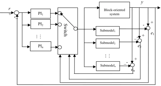
integral coefficients for the ith PI controller, respectively. The m PI controllers are scheduled by hard switching according to the operating conditions, as is displayed in Fig. 3.
The design of a Multi-PI controller for a block-structured nonlinear system is summarized in the following steps:
Firstly, decompose the block-oriented nonlinear system into a set of linear subsystems through the included angle dividing method;
Secondly, design a PI controller for each linear subsystem according to Eqs. (18), (19);
Finally, schedule the PI controllers by hard switching in terms of the operating conditions.
Figure 3. Multi-PI control of a block-structured system
IV. SIMULATIONS
A. pH Process
The pH process is a typical Wiener type system where the material balance differential equations are almost linear and the equilibrium equation (titration curve) is a strong nonlinear static function. Consider the pH process described by Eq. (20), where the weak acid of acetic acid (CH3COOH) is titrated by the strong base of sodium hydroxide (NAOH). Simulation data are displayed in Table I. The material balance equations and the equilibrium equation are as follows [6]:
0
0
( )
( ( )) ( ) ( ) ( ) ( ( )) ( )
[ ]
[ ] [ ]
pH log([ ]) a
a a
b
b b
w a a
b
a dC t
V FC F u t C t
dt dC t
V u t C F u t C t
dt
K K C
H C
H K H
H +
+ +
+
⎧ = − +
⎪ ⎪
⎪ = − +
⎪ ⎨ ⎪
+ = +
⎪ +
⎪
⎪ = −
⎩
(20)
As is shown in Fig. 4, the pH process exhibits strong static nonlinearity (output nonlinearity). A single linear controller is not able to satisfy the control requirements. In the following, the proposed Multi-PI control method is employed. Firstly, divide the system by the included angle method, and two linear submodels are obtained (models are omitted for short of space). Their operating points are (u01, y01) = (0.05, 8.5609) and (u02, y02) =
(0.0565, 11.488), respectively. Then design a linear PI controller for each linear submodel. The parameters of the PI controllers are as follows:
PI1: KP1=0.003, KI1=0.0002;
PI2: KP2=0.16, KI2=0.012.
The two PI controllers are scheduled according to the operating condition to make a global controller for set-point tracking control and disturbance rejecting control.
The excellent closed-loop simulation results are shown in Fig. 5-6.
0.0455 0.05 0.055 0.06
6 7 8 9 10 11 12
u
y
Figure 4. The titration curve of pH process (static I/O map).
Switch
PI1
PIn
Submodel1 Block-oriented
system
Submodel2
Submodeln
…
…
+ - +
+ _-
_-
-_
+ r
e1
e2
en
y
PI2
…
…
TABLE I.
SIMULATION DATA OF PH PROCESS
Dissociation constant of water Kw 1.0×10⁻¹⁴
First dissociation constant of
CH3COOH Ka 1.8×10⁻⁵
Initial icon concentration of the
acid Ca0 0.02mol/L
Initial icon concentration of the
base Cb0 0.5mol/L
Reactor volume V 5L
Feed flow rate F 1L/min
0 5 10 15 20 25 30 35 40 45 50 6
8 10 12
y
Setpoint tracking response of pH system
0 5 10 15 20 25 30 35 40 45 50
0.02 0.04 0.06 0.08
time(sec)
u
u Ref y
Figure 5. Setpoint tracking control of pH process.
0 5 10 15 20 25 30
6 7 8 9
y
Disturbance rejection of pH system
0 5 10 15 20 25 30
0.044 0.046 0.048 0.05 0.052
time(sec)
u
u Ref y
Figure 6. Disturbance rejecting control of pH process.
Fig. 5 shows the set-point tracking response of the pH process under the designed Multi-PI controller. Obviously, the output follows the reference signal swiftly and accurately, no matter within one operating subspace or transition between neighbor subspaces. So the Multi-PI controller based on two linear submodels performs an excellent set-point tracking control task for this pH process.
Fig. 6 shows the disturbances rejecting response of the pH process under the Multi-PI controller. At time = 18sec, -9% unmeasured disturbance is added to the system. So we can see from Fig. 6, the output y strays away from the reference signal at time = 18sec. But it goes back to the neighborhood of the set-point quickly, and finally settles at the set-point. So the Multi-PI controller performs an excellent disturbance rejecting job, and satisfies the control requirements.
B. Heat-Exchanger
Consider a Heat Exchanger modeled by the following Hammerstein model [18]
2 3
4
( ) 31.549 41.732 24.201 68.634
x u u u u
u
= − + −
+ (21)
1 2
1
1 2
0.207 0.1764
( )
1 1.608 0.6385
z z
G z
z z
− −
−
− −
− =
− + (22)
where, x(k) is the static nonlinear intermediate variable, u(k) is the water flow rate, and y(k) is the water exit temperature. The input to the process is constrained between [0, 1]. The control objective is to keep the process output as close as possible to the reference signal.
The static input-output map is depicted in Fig. 7, from which it is clearly seen that the Heat Exchanger process exhibits strong static nonlinearity—input multiplicity. Thus, the usual nonlinearity inversion control method is not applicable to this Heat Exchanger process. Here in this paper, the Multi-PI control will be applied to it.
First, the process is divided into two linear subsystems through the included angle dividing method. The operating points are (u01, y01) = (0.17,-4.22), (u02, y02) =
(0.66, 3.4215). Design a PI controller for each linear system. The parameters of the two PI controllers are as follows:
PI1:Kp1=0.02; Ki1=0.01;
PI2:Kp2=0.012; Ki2=0.0043.
Combine the two PI controllers as a global control by hard switching. And this Multi-PI controller will be applied to the Heat Exchanger process in the following.
Fig. 8 displays the Heat-Exchanger’s closed-loop simulation of set-point tracking control under our designed Multi-PI controller. As is seen clearly, the output y follows the reference signal closely in the entire operating region. The fast, accurate, and smooth output response proves a good performance of the Multi-PI controller for set-point tracking control.
In Fig. 9, 4% disturbance v is added to the system at time = 80, and v is removed at time = 140. The response is quite satisfactory. When v appears at time = 80, the controller brings the output y back to the set-point quickly and precisely. When v vanishes at time = 140, the Multi-PI controller can also regulate the output y easily.
Figs. 8-9 illustrate the effectiveness of the Multi-PI controller for the Heat Exchanger process with input multiplicity.
0 0.1 0.2 0.3 0.4 0.5 0.6 0.7 0.8 0.9 1 -10
0 10 20 30 40 50 60
u(k)
y(
k)
0 20 40 60 80 100 120 140 160 180 200 0
20 40 60
y
Setpoint Tracking Response of Heat Exchanger
0 20 40 60 80 100 120 140 160 180 200 0
0.2 0.4 0.6 0.8 1
time
u
y Ref
u
Figure 8. Set-point tracking control of Heat Exchanger.
0 20 40 60 80 100 120 140 160 180 200
0 20 40 60
y
Disturbance Rejection of Heat Exchanger
0 20 40 60 80 100 120 140 160 180 200
0 0.2 0.4 0.6 0.8 1
time
u
u y Ref
Figure 9. Disturbance rejecting of Heat Exchanger.
V. CONCLUSIONS
Block-structured models have proved to be popular in modeling industrial processes for their special and convenient structures, which facilitate the system analysis and synthesis. However, the general nonlinearity inversion control method and other control methods for block-structured models needs the static element to be invertible, which is not always satisfied, especially for systems with input or/and output multiplicity. Moreover, the nonlinearity inversion method may lead to a degraded performance. To improve the situation, a special purposed Multi-PI control method is proposed for block-structured systems in this paper. In our method, based on the special structure of block-structured systems, an included angle dividing algorithm is employed to decompose a block-structured system into a set of linear subsystems, then a nonlinear control problem is decomposed into a set of linear control ones, to which the classic PI control strategy can be easily applied. Thus, a complex problem is solved in an easy way. Two
benchmark systems are studied. Simulations illustrate the effectiveness of the Multi-PI controller.
ACKNOWLEDGMENT
This work is supported partially by the NSF (61104079, 60974023) of China, partially by the Fundamental Research Funds for the Central Universities, and partially by the Doctors’ Funds (B2011-007) of Henan Polytechnic University.
REFERENCES
[1] R. K. Pearson, “Nonlinear empirical modeling techniques,” Computers and Chemical Engineering, vol. 30, no.5 pp.1513-1528, May 2006.
[2] S. J. Norquay, A. Palazoglu, and J. A. Romagnoli, “Model predictive control based on Wiener models,” Chem. Eng. Sci., vol. 53, no.5, pp. 75-84, May 1998.
[3] K. P. Fruzzetti, A. Palazoglu, and K. A. McDonald, “Nonlinear model predictive control using Hammerstein models,” Journal of Process Control, vol. 7, no.4, pp. 31-41, April 1997.
[4] L. Jia, M. S. Chiu, and S. S. Ge, “A noniterative neruo-fuzzy based identification method for Hammerstein processes,” Journal of Process Control, vol. 15, no. 3, pp. 749-761, March 2005.
[5] G. Harnischmacher and W. Marquardt, “Nonlinear model predictive control of multivariable processes using block-structured models,” Control Engineering Practice, vo. 15, no.6, pp.1238-1256, December 2007.
[6] S. Sung and J. Lee, “Modeling and control of Wiener-type processes,” Chemical Engineering Science, vol. 59, no.10, pp. 1515-1521, October 2004.
[7] H. H. J. Bloemen, T. J. J. van den Boom, and H. B. Verbruggen, “Model-based predictive control for Hammerstein systems,”. Proc. of 39th IEEE Conference on Decision and Control, Sydney, Australia, pp. 4963-4966, December, 2000.
[8] Y. M. Hlaing, M. S. Chiu, S. and Lakshminarayanan, “Modelling and control of multivariable processes using generalized Hammerstein model,” Chem. Eng. Res. Des. vol. 85, no.4, pp. 445-454, April 2007.
[9] R. K Pearson, M. Pottmann, “Gray-box identification of block-oriented nonlinear models,” Journal of Process Control, vol. 10, no.3, pp. 301-315, March 2000.
[10] Q. Chen, L. Gao, R. A. Dougal, and S. Quan, “Multiple model predictive control for a hybrid proton exchange membrane fuel cell system,” Journal of Power Sources, vol. 19, no. 5, pp. 472-482, May 2009.
[11] J. Du, X. Zhang, and C. Song, “Multi-PID Control of Hammerstein Systems with Input Multiplicity,” in the 30th Chinese Control Conference, Yantai, China, pp. 303-306, July 22-24, 2011.
[12] Y. Liu, Y. Gao, Z. Gao, H. Wang, and P. Li, “ Simple Nonlinear Predictive Control Strategy for Chemical Processes Using Sparse Kernal Learning with Polynomial Form,” Ind. Eng. Chem. Res.,vol. 49, no.7, pp. 8209-8218, July 2010.
[13] O. Galán, J. A. Romagnoli, A. Palazoglu, and Y. Arkun, “Gap metric concept and implications for multilinear model-based controller design,” Ind. Eng. Chem. Res., vol. 42, no.6, pp. 2189-2197, June 2003.
[15] J. Du, C. Song, and P. Li, “Multilinear model control of Hammerstein-like systems based on included angle dividing method and the MLD-MPC strategy,” Industrial and Engineering Chemical Research, vol. 48, no.1, pp. 3934-3943, January 2009.
[16] O. Galán, J. A. Romagnoli, and A. Palazoglu, “Real-time implementation of multi-linear model-based control strategies-an application to bench-scale pH neutralization reactor, ” Journal of Process Control, vol. 14, no.7, pp. 571-679, July 2004.
[17] J. Du and C. Song, “An Included Angle Based Nonlinearity Measure for Hammerstein-like Systems,” in the 2011 International Conference on Electric Information and Control Engineering, Wuhan, China, pp. 152-155, April 15-17, 2011.
[18] E. Eskinat and S. H. Johnson, “Use of Hammerstein models in identification of nonlinear systems,” AIChE Journal, vol.37, no.5, pp. 255-266, May 1991.
[19] J. Li, Y. Lu, Z. Ji, H. Pei, “Constrained Optimal Controller Design of Aerial Robotics Based on Invariant Sets”,
Journal of Software, vol. 6, no.2, pp.193-200, Feb. 2011.
[20] J. Wang, M. Huang, H. Wang, L. Guo, W. Zhou, “Research on Detectable and Indicative Forward Active Network Congestion Control Algorithm”, Journal of Software, vol. 7, no.6, pp. 1195-1202, June 2012.
[21] P. Zhang, X. Hao, H. Li, W. Xu, “Novel Learning Algorithm for System Model of Traditional Chinese Drug Fumigation”, Journal of Software, vol. 6, no.6, pp. 1017-1024, June 2011.
[22] W. Jiang, “The Application of the Fuzzy Theory in the Design of Intelligent Building Control of Water Tank”, Journal of Software, vol. 6, no.6, pp. 1082-1088, June 2011.
[23] Q. Wang, S. Ge, L. Jia, Pinning Control of Complex
Network by a Single Controller, Journal of Software, vol. 7,
no.10, pp.2258-2262, Oct. 2012.
Jingjing Du was born in Henan province, China, in 1982. She received the B.S. degree in industrial automation from China Jiliang University in June 2005, and the Ph.D. degree in control science and engineering from Zhejiang University in June 2010.
From 2007 to 2009, she was a teaching assistant in the Department of Control Science and Engineering, Zhejiang University. From July 2010 until now, she is an Associate Professor in the School of Electrical Engineering and Automation, Henan Polytechnic University, China. Her research interests are in multi-model control of nonlinear systems, nonlinearity measure, and hybrid system control.
Chunyue Song received the B.S. degree in Automation of Chemical Engineering and Ph.D. degree in control science and engineering from Zhejiang University, Hangzhou, China, in 1994 and 2003, respectively.