The Impact of Conditional Cash Transfer Programs Under Risk-Sharing Arrangements: Schooling and Consumption Smoothing in Rural Mexico

University of Pennsylvania

ScholarlyCommons

Publicly Accessible Penn Dissertations

1-1-2014

The Impact of Conditional Cash Transfer Programs

Under Risk-Sharing Arrangements: Schooling and

Consumption Smoothing in Rural Mexico

Eun-young Shim

University of Pennsylvania, [email protected]

Follow this and additional works at:http://repository.upenn.edu/edissertations

Part of theLabor Economics Commons

Recommended Citation

Shim, Eun-young, "The Impact of Conditional Cash Transfer Programs Under Risk-Sharing Arrangements: Schooling and Consumption Smoothing in Rural Mexico" (2014).Publicly Accessible Penn Dissertations. 1440.

The Impact of Conditional Cash Transfer Programs Under Risk-Sharing

Arrangements: Schooling and Consumption Smoothing in Rural Mexico

Abstract

This paper develops and estimates a model of informal risk sharing with limited commitment that

incorporates children's school attendance choices. The model is estimated using Mexican rural villages data from the PROGRESA experiment and is used to analyze how the presence of informal risk sharing influences schooling and child labor choices, as well as the effectiveness of conditional cash transfer (CCT) programs. In particular, I compare the outcomes (schooling, child labor, and consumption) generated under the informal risk-sharing model with those that would be obtained, forcing households to make choices under autarky. I evaluate the effect of alternative program designs that were also considered in other papers which did not incorporate inter-household transfers. I find that the number of years of schooling completed at age 18 is 0.5 years lower under autarky than with risk sharing. Also, the effect of CCT on schooling outcomes and welfare of households is larger under autarky than under risk sharing, and CCT increases consumption volatility under risk sharing, especially among households with young children who are subject to the future program benefit.

Degree Type

Dissertation

Degree Name

Doctor of Philosophy (PhD)

Graduate Group

Economics

First Advisor

Kenneth I. Wolpin

Keywords

CCT, Conditional cash transfer, Informal risk sharing, limited commitment, PROGRESA

Subject Categories

THE IMPACT OF CONDITIONAL CASH TRANSFER PROGRAMS

UNDER RISK-SHARING ARRANGEMENTS: SCHOOLING AND

CONSUMPTION SMOOTHING IN RURAL MEXICO

Eun-young Shim

A DISSERTATION

in

Economics

Presented to the Faculties of the University of Pennsylvania

in

Partial Fulfillment of the Requirements for the

Degree of Doctor of Philosophy

2014

Supervisor of Dissertation

Kenneth I. Wolpin

Walter H. and Leonore C. Annenberg Professor in the Social Sciences

Graduate Group Chairperson

Goerge J. Mailath

Walter H. Annenberg Professor in the Social Sciences and Professor of Economics

Dissertation Committee

Flavio Cunha, Assistant Professor of Economics Hanming Fang, Professor of Economics

THE IMPACT OF CONDITIONAL CASH TRANSFER PROGRAMS UNDER

RISK-SHARING ARRANGEMENTS: SCHOOLING AND CONSUMPTION

SMOOTHING IN RURAL MEXICO

COPYRIGHT

2014

Eun-young Shim

This work is licensed under the

Creative Commons

Attribution-NonCommercial-ShareAlike 3.0

License

To view a copy of this license, visit

DEDICATION

I dedicate my dissertation to my family. This work would not have been possible

ACKNOWLEDGMENT

I am greatly indebted to Kenneth Wolpin, Flavio Cunha, Hanming Fang, and Dirk

Krueger for their invaluable guidance and support. I have greatly benefited from

discus-sion with Jere Behrman, Andrew Clausen, Harold Cole, Susumu Imai, Robert Jensen,

Yena Park, Petra Todd, and Shing-Yi Wang. I thank the Federal Reserve Bank of St.

Louis for its hospitality and support during my visit. I also thank seminar participants

at Penn empirical micro workshop and empirical micro lunch, Federal Reserve Bank of

St. Louis, and SWUFE International Workshop on Applied Microeconomics in 2012 for

helpful comments and suggestions. This research was supported in part by the National

Science Foundation through XSEDE resources provided by the XSEDE Science

ABSTRACT

THE IMPACT OF CONDITIONAL CASH TRANSFER PROGRAMS UNDER

RISK-SHARING ARRANGEMENTS: SCHOOLING AND CONSUMPTION

SMOOTHING IN RURAL MEXICO

Eun-young Shim

Kenneth I. Wolpin

This paper develops and estimates a model of informal risk sharing with limited

com-mitment that incorporates children’s school attendance choices. The model is estimated

using Mexican rural villages data from the PROGRESA experiment and is used to analyze

how the presence of informal risk sharing influences schooling and child labor choices,

as well as the effectiveness of conditional cash transfer (CCT) programs. In particular, I

compare the outcomes (schooling, child labor, and consumption) generated under the

in-formal risk-sharing model with those that would be obtained, forcing households to make

choices under autarky. I evaluate the effect of alternative program designs that were also

considered in other papers which did not incorporate inter-household transfers. I find that

the number of years of schooling completed at age 18 is 0.5 years lower under autarky

than with risk sharing. Also, the effect of CCT on schooling outcomes and welfare of

households is larger under autarky than under risk sharing, and CCT increases

consump-tion volatility under risk sharing, especially among households with young children who

Contents

1 Introduction 1

2 Model 7

2.1 Set-up . . . 8

2.1.1 Village and Household Demographics . . . 8

2.1.2 School Grade Completion and Activity Choices of Children . . . 9

2.1.3 Type Probability . . . 10

2.1.4 Income Process . . . 10

2.1.5 Preference . . . 11

2.2 Risk Sharing Problem . . . 13

2.2.1 State Space . . . 13

2.2.2 Autarky . . . 13

2.2.3 Risk Sharing with Limited Commitment . . . 14

2.2.4 The agent’s Problem . . . 16

3 Data 19 4 Estimation 28 4.1 Parameter estimates . . . 31

4.1.1 Income, wage, and type process parameters . . . 32

4.1.2 Preference Parameters . . . 34

4.2 Model fit . . . 36

5 Counterfactual Analysis 40 5.1 Risk Sharing and Autarky . . . 41

6 Conclusion 50

A Autarky Problem 53

B Solution Algorithm for the Agent’s Problem 55

C Household Consumption and Income Variables 62

C.1 Consumption . . . 62

List of Tables

1 PROGRESA monthly education grant schedule in 1998 . . . 20

2 Proportion of children making transitions into or out of school . . . 21

3 Reasons for not attending school . . . 22

4 Percentage of households having experienced various shocks . . . 24

5 Informal financial activities in PROGRESA villages . . . 25

6 Summary statistics . . . 27

7 Parameter estimates: income process . . . 32

8 Parameter estimates: child wage process . . . 33

9 Parameter estimates: type process . . . 34

10 Parameter estimates: preference . . . 35

11 Actual and Predicted Mean Parental and Household Income . . . 37

12 Actual and predicted log parental and household income variance . . . 38

13 Actual and predicted parental income by mother’s completed school grade . . . 38

14 Actual and predicted moments by age . . . 39

15 Actual and predicted consumption, proportion attending school and stay-ing home, mean wage by income quartile . . . 40

16 Actual and predicted correlation between household income and con-sumption . . . 40

17 Outcomes under risk sharing and autarky . . . 42

21 The effect of CCT on income, consumption, and welfare outcome under

risk sharing . . . 46

22 The effect of CCT on schooling outcome under autarky . . . 47

23 The effect of CCT on income, consumption, and welfare outcome under

autarky . . . 48

24 (a) Fraction of children attending school and (b) mean household

con-sumption under autarky by cross-sectional parental-income states . . . 49

25 Effect of CCT with completed grade at age 12 fixed at 2nd grade,

benefi-ciary households only . . . 49

26 Income by source (in 1998 pesos) . . . 64

List of Figures

1 School enrollment rate and completed school grade by age . . . 21

2 Child labor in PROGRESA villages . . . 23

3 Estimated distribution over discretized income states . . . 41

1

Introduction

Over recent decades, many developing countries have adopted conditional cash transfer

(CCT) programs as a new approach to reducing poverty and increasing the human capital

of the next generation. These programs give cash grants to poor households conditional

on children’s school attendance. In 1997, the Mexican government initiated one of the

first programs, which is called the Programa de Educación, Salud y Alimentación, or

PROGRESA (the current program is named Oportunidades), and similar programs were

adopted throughout Central and Latin America and, more recently, in South East Asia and

Africa (Fiszbein and Schady, 2009). The randomized implementation of PROGRESA

and its collection of extensive data offered researchers unique opportunities to evaluate

the program’s effectiveness and to study alternative program subsidy designs (Attanasio,

Meghir, and Santiago, 2012; Behrman, Sengupta, and Todd, 2005; Schultz, 2004, Todd

and Wolpin, 2006, among others).

Most of the existing studies of the effects of CCT programs on child schooling have

modeled the behavior of households without regard to transfers between households and

have focused on short-term program effects. An important reality of the lives of poor

families in developing countries is that, in the absence of formal lending opportunities,

they manage income risk through transfers among relatives and neighbors, often referred

to as “informal risk sharing” (see Fafchamps, 2008, for the survey). There is evidence that

public transfers that are targeted to specific groups, such as old age pension programs or

conditional cash transfers, are shared by others through informal risk sharing and crowd

out existing informal transfers (Albarran and Attanasio, 2003; Angelucci and Di Giorgi,

2009; Dercon and Krishnan, 2003; Jensen, 2004). The treatment effects estimated with

experimental treatment and control groups, such as those obtained under the PROGRESA

stud-ies that develop structural models to evaluate the effects of alternative program designs,

and which assume that households face only household-level income constraints, may not

fully capture program effects.1 Moreover, most of the CCT literature focuses on

short-term program effects, as the data are usually only available for a few years. The

longer-term effects may be different from observed short-longer-term effects, as households adjust their

risk-sharing behavior in response to both the transfers and to additional changes in the

level and variability of income arising from children’s increased schooling.2 At the

sub-sistence level, managing income risk is crucial for the ability of households to meet their

daily basic needs, and thus, understanding the change in informal risk sharing behavior is

important in evaluating the welfare effect of the CCT programs. Also, financial constraint

is an important determinant of a child schooling and labor choice, and these outcomes

may respond to the change in the availability of informal transfers (Jacoby, 1994; Jacoby

and Skoufias, 1997).

This paper develops and estimates a model of informal risk sharing with limited

com-mitment that incorporates children’s school attendance choices. My model builds on and

extends the earlier informal village risk-sharing models introduced in Townsend (1994),

on the limited commitment framework developed in Ligon, Thomas, and Worrall (2000,

2002), Laczó (2011), and on the large economy model of Krueger and Perri (2011). The

model is estimated using data from the PROGRESA experiment and is used to analyze

how the presence of informal risk sharing influences the effectiveness of CCT programs.

In particular, I compare the treatment outcomes (schooling, consumption, and income)

generated under the informal risk sharing model with those that would be obtained

forc-ing households to make choices under autarky. I quantify the effect of informal risk

1_{The notable exceptions are Angelucci, Di Giorgi, Rangel, and Rasul (2010), and Angelucci, Di Giorgi,}

and Rasul (2012).

2_{Attanasio and Rios-Rull (2000) and Krueger and Perry (2006, 2011) show that lower income variability}

sharing and study the mechanisms through which risk sharing promotes schooling

attain-ment. I evaluate the effect of alternative program designs which were also considered in

other papers that did not incorporate inter household transfers (Attanasio, Meghir, and

Santiago, 2012; Todd and Wolpin, 2006).

In the model, I consider a closed village economy, populated by a continuum of

over-lapping generations of households who make a collective decisions about (1) the size of

the transfers given to or received by each household, and (2) which households send their

child to school. The arrangement is based on the households’ voluntary incentive to share

their income with others, and hence, the arrangement is made in such a way that the

fu-ture gain from staying in the arrangement relative to autarky is sufficient to compensate

for the amount households have to share in the current period. Incorporating this so-called

limited-commitment constraint, the arrangement endogenously responds to the expected

and the actual changes in the autarky value driven by government transfers.3

Households begin their lifecycle as a married couple, and, with some probability,

a child birth occurs. Children are eligible to attend school between ages of 6 and 18,

during which time they can either choose to stay home, attend school, or work for a

child labor wage. There is a utility cost of returning to school after an interruption of

school attendance. Parents’ income and child wage offers are exogenous and stochastic,

and household income is pooled. Children aged 19 and over are assumed to work, and

household income depends on child schooling attainment. Household income may also

differ across households according to permanent unobserved types of parents and children

which are incorporated into the model.

Households have an incentive to participate in risk sharing mainly for two reasons.

First, households are risk averse and want to smooth their consumption against future

3_{Albarran and Attanasio (2003) find evidence that the limited-commitment constraint is present in these}

shocks. Second, schooling interruptions are costly, so parents have an incentive to keep

their child in school even in periods where they receive negative income shocks.

Directly solving for the allocation for all households for all possible states is not

fea-sible. However, a solution can be found by solving a contract between a household and an

infinitely-lived, risk-neutral agent (see Atkeson and Lucas, 1992, 1995; and Krueger and

Perri, 2011). The advantage of this algorithm is that it reduces the original problem to a

recursive cost minimization problem of the risk-neutral agent, who is committed to deliver

a certain level of lifetime utility (which is promised in the contract) to a given household

without having to track the distribution of the allocations received by all households. This

approach requires assuming that the village economy is stationary.

In 1997, the Mexican government launched a large-scale cash transfer program

tar-geting the rural poor. The program, which was called PROGRESA, paid a cash grant

to mothers upon the school attendance of their children, and detailed panel data were

collected to evaluate the program. The data includes 25,000 households in 506 villages,

and all households in selected villages were surveyed. Thus, I observe the information of

all households that would participate in the risk-sharing arrangement. The data contain

detailed information about household income and consumption and also about the age,

completed school grade, main activity, and wage income earned by each household

mem-ber. Among the 506 villages, 186 were selected as control villages, and the CCT program

for them was delayed until the end of 1999. In estimation, I use the 11 largest control

vil-lages, which have more than 100 households each.4 The model parameters are estimated

by the simulated method of moments, matching the observed income, consumption, and

child activity choices predicted by the model to those in the PROGRESA data.

4_{I restrict the sample to large control villages for two reasons. First, the model assumes a continuum}

Based on the estimated model, I find that informal risk sharing promotes more

reg-ular school attendance for children and helps households smooth consumption against

income shocks. When households engage in risk sharing, school attendance and child

labor choices are not responsive to parental income fluctuations, whereas in autarky, they

are significantly affected by them. A temporary decrease in parental income leads to a

school enrollment rate that is 12 percentage points lower under autarky than with risk

sharing. Due to high estimated adjustment costs, only a small fraction of children return

to school once schooling is interrupted. Under autarky, the impact of a low income shock

in one year is persistent. I find that the amount of schooling completed by children by the

age of 19 is 0.47 years less under autarky than with risk sharing.

I also introduce a CCT program that is similar to PROGRESA to the estimated model

with and without risk sharing and find that the effect of the CCT program on schooling

outcomes and household welfare is larger under autarky than under risk sharing.

Com-pared to when there is no CCT program, the amount of schooling completed by children

by the age of 19 increases by 1.12 years under autarky and by 0.85 years under risk

shar-ing. School enrollment rate increases by 23 percentage points under autarky and by 19

percentage points under risk sharing. One of the benefits of CCT is that it mitigates the

effect of negative income shocks on household consumption and school attendance. This

effect, however, is negligible under risk sharing because the allocations under risk

shar-ing were close to efficient allocations even without the CCT. Moreover, the correlation

between household income and consumption under risk sharing increases by 13 percent

compared to when there is no CCT. This is because beneficiary households can rely on

the CCT benefit if inter-household transfer becomes unavailable, and this weakens their

voluntary participation incentive to remain in the risk-sharing arrangement. This offsets

some of the welfare gains from the CCT under risk sharing.

program, especially to Attanasio, Meghir, and Santiago (2012) and Todd and Wolpin

(2006), both of which use a structural modeling approach to model schooling decisions.

Both papers evaluate the effects of alternative policies that involve reallocating program

benefits among households. My modeling framework is much different in that it is an

equilibrium model that allows for transfers among households. I examine how policy

effects differ in an environment where households make or receive transfers and jointly

make schooling decisions relative to an autarky environment.

Other closely related papers are Angelucci, Di Giorgi, Rangel, and Rasul (2010) and

Angelucci, Di Giorgi, and Rasul (2013). These papers find that the PROGRESA program

was effective in increasing child schooling only for the households which have extended

family network ties within the same village, suggesting that informal risk sharing plays

an important role. This paper takes an alternative approach by developing and estimating

a model that allows the amount of risk sharing within each village to be endogenously

determined. This approach is more flexible when it comes to an evaluation of alternative

policies by allowing risk sharing outcomes to vary depending on the nature of each policy.

Several papers structurally estimate dynamic risk-sharing models with limited

com-mitment using village-level data. Ligon, Thomas, and Worrall (2002) find that estimated

model explains the consumption dynamics in rural Indian villages better than alternative

models, including autarky and a static risk-sharing model. Laczó (2011) formally

ap-plies statistical tests to different risk sharing regimes using the same Indian villages data

and finds that limited commitment with heterogenous preference outperforms alternative

models. She also studies the effect of a counterfactual public cash transfer policy on the

risk-sharing arrangement. Their analysis is confined to consumption risk sharing and does

not incorporate schooling or any other investment decision.

Ligon, Thomas, and Worrall (2000) consider a limited-commitment risk-sharing model

show that the existence of savings helps to smooth aggregate shocks, but it may decrease

welfare by making the outside option more attractive. My model does not incorporate

savings (very few households in the data have savings), but I instead incorporate the

schooling decision as a form of investment. Schooling differs from savings or other

phys-ical capital because schooling investments have to be made continuously during a specific

interval of the lifecycle, and households receive direct utility from schooling. An

impli-cation of my model is that households which want to invest in schooling demand more

risk sharing.

This paper is also related to a large literature on informal risk sharing in rural village

economies that originated with Townsend (1994), who studied risk sharing among

vil-lagers in rural India. Since then, numerous papers have documented similar behaviors

in many different countries (Dercon and Krishnan, 2003; Fafchamps and Lund, 2003;

Kinnan, 2011; Mazzocco and Saini, 2009; and Morduch, 1995, among others). Cox and

Fafchamps (2007) and Fafchamps (2008) provide extensive reviews of the literature on

informal risk sharing and evidence of crowding out of public transfers found in the

liter-ature.

The rest of the paper is organized as follows. The model is presented in section 2.

Sec-tion 3 provides a descripSec-tion of the data. SecSec-tion 4 introduces estimaSec-tion procedure and

results. Section 5 presents the description and the analysis of counterfactual experiments,

and section 6 concludes.

2

Model

In the following subsections I first set up the model environment, including the village and

household demographics and the choices and risks which these households face. Then I

an efficient allocation under risk sharing, I introduce an agent who mediates interaction

among households. The agent’s problem is presented at the end of this section.

2.1

Set-up

2.1.1 Village and Household Demographics

I consider a closed village economy, populated by a continuum of overlapping generations

of households. The life of a household begins without a child. A household is endowed

with some level of lifetime utilityω0 and unobserved type ptype. Fertility shocks arrive

once a year, and a childbirth occurs with probabilityπb. Once a child is born, the fertility

process ends. Children between the ages of 6 and 18 are eligible to attend school. After a

child reaches age 19, he or she is no longer eligible to attend school, and instead always

works and contributes to household income. Children in this stage also may permanently

leave their households and stop contributing to household income with probability πm.

This event is called a “migration” in the remaining of the paper. Households in this stage

(i.e., a household whose grown-up child is no longer present), whose grown-up child is

no longer present, stochastically dissolve with probability πd, after which they do not

consume nor obtain any utility. Dissolved households are replaced by new households so

as to keep the village demography stationary. At any given time period, each village is

populated by households in different stages in their life cycle.

A period in the model equals one school semester (six months), and there are two

periods within one year (fall and spring semester). All demographic transitions including

birth, migration, dissolution, and the evolution of a child’s age occur once a year, in the

beginning of the fall period.5

5_{The model assumes that each household has at most one child. This is restrictive because households}

2.1.2 School Grade Completion and Activity Choices of Children

Children between ages 6 and 11 always attend school. Between ages 12 and 18, they either

stay home, attend school, or work for a wage. These activity choices are mutually

exclu-sive. I defined_tj=1 if alternative jis chosen in periodt where j∈ {home, school, work}.

If alternative j is not chosen,d_tj=0. dt denotes a vector{dthome,dtschool,dtwork}. School

enrollment choices for a child are made twice a year, at the beginning of the fall and the

spring semesters.

Although children under age 12 always attend school, they may fail their school grade

and need to repeat the year. Rather than modeling that each child completes or fails a

grade every year, the model determines each child’s completed grade at the time the child

turns 12. Define X_tc to be the completed grade of a child at the beginning of t. The

probability thatX_tc=X forX =0, ...,6 is denoted byπ_gr12(X,ptype):

Pr(X₁₂c =X) = π_gr12(X,ptype)

and the probability sums up to 1,∑6_X=0πgr12(X,ptype) =1.

Between ages 12 and 18, school grade completion is determined at the end of

ev-ery spring semester. The probability that a grade is completed by a child is a

func-tion of school attendance choices in that year, d_tschool₋₁ and d_tschool, and is denoted by

πgr(dtschool,dtschool−1 ).

2.1.3 Type Probability

The probability that a parent or a grown-up child whose completed grade is X is

high-income type is given by:

Pr(type=high|X) = exp(Xγ)

1+exp(Xγ),

where

Xγ ≡γo+γXX+γ61{X ≥6}+γ91{X≥9}+γ121{X ≥12}.

2.1.4 Income Process

Households face a stochastic income process. This is a major source of risk in the model.

Before a child becomes 12 years of age, his or her parents are the household’s only income

earners. The parental income process is given by the following:

log

y_ip_,v,t

=β_vp+µ_ptypep _i+ε_ip_,v,t , ε_ip_,v,t∼N 0,σ_p2_,v,

where β_vp is a village fixed effect, µ_ptypep _i denotes an unobserved parental component

type ptype_i, andε_ip_,v,t is an idiosyncratic shock that is independent over time and across

households. Letadenote the age of a child. The child’s wage process between ages 12

and 18 is given by the following:

log(wi,v,t(a)) =β_aw+ε_iw_,v,t,ε_iw_,v,t∼N(0,σ_w2),

where β_aw is an age specific mean and ε_iw_,v,t is an idiosyncratic shock. When a child is

between ages 12 and 18, household income,yh_i,v,t, is the sum of the parental income and

yh_i,v,t=y_ip_,v,t+wi,v,t1{dtwork=1},

ε_ip_,v,t andε_iw_,v,t are independent of each other. As a child reaches age 19, both the parents

and child jointly generate household income:

logyh_i,v,t=β_vh+µ_ptypep _i+µ_ctypec _i+ε_ih_,v,t , ε_ih_,v,t∼N 0,σ_h2_,v,

whereµ_ctypec _i denotes an unobserved type component of a child of typectypei. As parents

and grown-up child start to jointly generate household income, both the parental and the

child type enter the process. If there is no child or a child is below age 12,yh_i,v,t=y_ip_,v,t.

2.1.5 Preference

The period utility of household is derived from household consumption, completed school

grade and activity choices of a child:

u_i,t =uχ(χi,t) +uX(Xic,t) +uschool(dischool,t−1 ,dischool,t ,ai,t,Xic,t) +uwork(dworki,t ,ai,t), (1)

where

u_C(χi,t) =

χ_i1−_,t η−1

1−η ,

andχi,t is a composite good of household consumption and utility derived from the child

leisure given by

χi,t=ci,t+ (κhome,a+ξ)1{dihome,t =1},

with household consumption c_i,t, utility from the child’s leisure, κhome,a and ξ, where

logξ ∼N(0,σ2

ξ). Note thatκhome,a is age-specific. The utility from leisure can be

Households are risk averse overχi,t, and their period utility is represented by the constant

relative risk aversion utility function with risk aversion parameterη. uX(X_ic_,t)denotes the

utility from the completed school grade,X_ic_,t:

u_X(X_ic_,t) =κ61{Xic,t≥6}+κ91{Xic,t≥9}+κ121{Xic,t≥12}.

u_school(d_i,t−1,di,t,ai,t,X_ic_,t)denotes the utility cost of attending school:

u_school(d_i,t−1,d_i,t,a_i,t,X_ic_,t) = κgap11{dischool,t =1,ai,t−6−Xic,t >0} + κgap61{dischool,t =1,ai,t−6−Xic,t ≥6}

+ κgap91{dischool,t =1,ai,t−6−Xic,t ≥9} (2) + κprev1{dischool,t−1 =0,dischool,t =1}

The top three terms on the right hand side of the equation (2) capture the utility cost

of attending school when a child is behind the standard school grade for his or her age

(ai,t−6) by at least 1 year, more than 6 years, and more than 9 years, respectively. The

fourth term captures the cost of attending school when a child did not attend the school in

the previous period.

The last term of (1) captures the age-specific cost of working for a wage:

uwork(diwork,t ,ai,t=a) =κwork,a1{diwork,t =1}

2.2

Risk Sharing Problem

In this subsection, I formally define efficient allocations under risk sharing with limited

commitment and present the agent’s problem in a recursive formulation. Recall that the

outside option of households is to live under autarky. Therefore, to characterize the

vol-untary participation constraint, I first introduce the autarky problem.

2.2.1 State Space

Let us denote a vector of shocks received by householdiin periodt bysi,t. si,t includes

stochastic events affecting demographic transition (birth, migration, and dissolution),

parental income, child wage, leisure preference, grade completion. A history of s_i,t up

to periodτ is denoted bysτ_i. DefineΩi,τ to be a state that householdiarrived in at the

be-ginning of periodτ, consisting ofsτ_i and demographic characteristics including the initial

ex-ante lifetime utilityω0and the type of parents and a child,ptypeandctype:

Ωi,τ ={ω0,ptypei,ctypei,sτi,ai,τ,di,τ−1,Xic,τ}.

Also, denote the set of allΩi,τ that can be reached with a positive probability in periodτ

asΩτ.

2.2.2 Autarky

Under autarky, households make an optimal choice given their household budget

con-straint,ci,t =yh_i,t. The only choice involved under autarky is a child activity choice. The

discounted present lifetime utility of householdiwhich arrivedΩi,tin periodt is denoted

2.2.3 Risk Sharing with Limited Commitment

Households have an incentive to participate in risk sharing for two reasons. First,

house-holds are risk averse and want to smooth their consumption against future shocks.

Sec-ond, schooling interruptions are costly, so parents have an incentive to keep their child in

school even in periods where they receive negative income shocks. To manage income

risk, households participate in a risk-sharing arrangement where households pool their

income and make a collective decisions about (1) the size of the inter-household

trans-fers given to or received by each household, and (2) which households send their child to

school.

Households opt out to autarky unless they obtain at least as much utility as they

would without any risk sharing. Also, there is no means by which to enforce this

in-formal contract among the households. The decision whether to remain in or leave the

arrangement is made by each household in the beginning of each period after s_i,t is

re-alized. The only exception is for the households whose child is between ages 12 and

18. For these households, elements ins_i,t are realized sequentially. At the beginning of

each period, εp is realized first, and then{ξ,εw} follows. The decision whether to

re-main in the arrangement is made after the realization of εp but before that of{ξ,εw}.

Thus, they remain in the arrangement if and only if the utility from staying in the

ar-rangement is at least as much as the utility obtained under autarky in expectation over

possible{ξ,εw}realizations.6 For all households, the decision to remain in the

arrange-ment, once made, binds until the next periodεpis realized. It is assumed that the entire

arrangement breaks down if at least one household chooses to leave the arrangement, and

6_{If the participation constraint must be satisfied after{ξ,}

εw}is realized, the dimension of the problem

substantially increases, which makes the computation too costly. This is because the state-contingent utility

promise has to be made for all possible combinations of{ξ,εw}, whereas with the current assumption, there

hence, the allocation is constrained to keep every household within the arrangement in

every state in every period. An allocation under the risk sharing arrangement is denoted

by(c,d)≡ {{ci,t(Ωi,t),di,t(Ωi,t)}Ωi,t∈Ωt} ∞ t=0.

Defineu(Ωi,τ,c,d)to be the period utility of householdiin periodτ under allocation (c,d). The constraint to keep households in the arrangement, which will hereafter be called a voluntary participation constraint (V P), are given by the following:7

u(Ωi,t,c,d) + ∞

∑

τ=t+1

δτ−tE_Ωi,

τ|Ωi,t,di,t(Ωi,t)[u(Ωi,τ,c,d)]≥U Aut₍

Ωi,t).

There is no village-level aggregate saving or borrowing technology. Thus, in every

period, the sum of the consumption of all households should not exceed the sum of income

of the households in the village. The village resource constraint(RC)is given by,

ˆ

Ωi,t∈Ωt

ci,t(Ωi,t)dΦt(Ωi,t)≤ ˆ

Ωi,t∈Ωt

yh_i,t(Ωi,t)dΦt(Ωi,t)∀t,Ωt,

whereΦt(Ωi,t)is a cumulative distribution function ofΩi,t over the supportΩt in period

t. Subject to(V P)and(RC), households in a village in periodtjointly maximize the sum

of their discounted present value of lifetime utility:

max

c,d

∞

∑

τ=t

δτ−tE_sτ_|st

(ˆ

Ωi,τ∈Ωτ

u(Ωi,τ,c,d)dΦτ(Ωi,τ)

)

.

An allocation(c,d)is efficient with respect toΦt if the allocation solves the problem

with(RC)holds at equality. As shown in Atkeson and Lucas (1992, 1995) and Krueger

7_{For the periods when a child is between age 12 and 18,(V P)is given by the following:}

E_st|εp (

u(Ωi,t,c,d) + ∞

∑

τ=t+1

δτ−tEΩi,τ|Ωi,t,di,t(Ωi,t)[u(Ωi,τ,c,d)]

) ≥E_st|εp

and Perri (2011), solving for efficient allocations reduces to a standard dynamic

pro-gramming problem. In order to use recursive techniques, however, allocations under a

risk-sharing arrangement have to be restricted to stationary allocations. An allocation is

stationary ifΦt =Φfor allt. Extending Krueger and Perri (2011), which considered an

endowment economy, the solution can be found by solving a dynamic contract between a

household and an infinitely-lived, risk-neutral agent as described in the next subsection.

2.2.4 The agent’s Problem

The constrained efficient allocation of risk-sharing arrangement is found by solving a

dynamic contract between a household and an infinitely-lived, risk-neutral agent who is

responsible for allocating resources to a given household. It is assumed that the agent has

an access to an outside financial market where he or she can borrow or save at a risk-free

interest rateR. A household is promised a certain level of lifetime utility in the contract.

The agent determines how much of the promised lifetime utility should be delivered as a

form of current consumption and how much should be postponed into the next period as

a utility promise. In this subsection, I set up the agent’s problem in a recursive form.

In the contract a household is promised a certain level of lifetime utility, ωt, which

will be called the “promised utility” throughout the remainder of the paper. The objective

of the agent is to find an allocation that minimizes the discounted sum of the cost of

delivering ωt. The agent chooses the current period utility, h, and the state-contingent

promise to be made in the next period,ωt+1(Ωt+1), along with a child’s activity choicedt

when it is relevant. DefineC(·)to be the inverse utility function that gives the amount of

consumption necessary to deliverh_t.

The agent’s problem for households whose child is above age 18 is equivalent to

(2011). For these households the agent’s problem is given by:

TV(ωt,Ωt) = min ht,{ωt+1(Ωt+1)}∀st+1

C(h_t) + 1

REΩt+1|Ωt[V(ωt+1(Ωt+1),Ωt+1)]

, (3)

subject to

ωt =ht+δEΩt+1|Ωt[ωt+1(Ωt+1)], (4)

ωt+1(Ωt+1)≥UAut(Ωt+1)∀Ωt+1. (5)

When a child is of ageaand the child’s activity choices are involved:8

V_a(ωt,Ωt) =min dt

n

V_a(ωt,Ωt|dthome=1),Va(ωt,Ωt|dtschool=1),Va(ωt,Ωt|dtwork =1)

o

where

V_a(ωt,Ωt|dt) = min h,{ωt+1(Ωt+1)}∀_st+1



 

 

C(h_t,d_t)−w_td_twork

+_R1E_{Ωt+1|Ωt,dt}[V_a+1(ωt+1(Ωt+1),Ωt+1)]

     , subject to

ωt =ht+δE_Ωt+1|Ωt,dt[ωt+1(Ωt+1)]∀Ωt+1

ωt+1(Ωt+1)≥EΩt+1|Ωt,dt

h

U_tAut₊₁(Ωt+1)

i

∀Ωt+1.

The interest rateRis endogenously determined at the level where the agent neither

bor-8_{The agent’s problem presented in this subsection is simplified. For example, I did not distinguish the}

rows nor saves, and thus,(RC)holds at equality.

The extension of Krueger and Perri (2011) to this setting is not trivial. It is commonly

known that introducing an investment choice to a limited-commitment model makes the

constraint set non-convex. This is because the investment choice affects the outside option

value (under the assumption that returns from investment are still accrued under autarky),

and the convex combinations of the choices of promised utility and the level of investment

jointly may not be contained in the constraint set. The agent’s problem considered here,

however, solves the minimization problem given a discrete activity choice. Thus, given an

activity choice, such a non-convexity issue does not arise, and the minimization problem

with respect to the future promised utilities is well-defined.

Major challenges in computation arise due to the presence in the problem of both

discrete child activity choices and continuous choice variables {ωt+1(Ωt+1)}Ωt+1. The

presence of the dynamic discrete choices makes value functions nondifferentiable and

nonconvex with respect to promised utility ωt in the neighborhood where the optimal

child activity choice changes from one to another. As the differentiable and

non-convex value functions in period t+1 enter the optimization problem in periodt, the

first order condition is not well defined. Unlike in a standard dynamic discrete choice

model where introducing many shocks convexifies the objective function, there is one

continuous choice variable that needs to be solved for each possible realization of shocks.

Grid searches are robust to the nonconvexity of the objective function; however, the

trade-off between the accuracy of the solution and the computation speed is large. The

ac-curacy of the solution is important to obtain a value forRthat satisfies the village resource

constraint. In numerical simulations, a coarse grid ofωt+1leads to failure to finding such

a value forR. With a grid ofωt+1that is refined enough to find an equilibriumR, the

com-putation takes an infeasible amount of time. Because of the non-differentiability of the

be applied.

Fortunately, Clausen and Strub (2013) provide an envelope theorem that is applicable

in this setting. According to their envelope theorem, regardless of the presence of

non-differentiable parts in an objective function, optimal solutions are always found in

dif-ferentiable parts of the objective function. Based on that envelope theorem, Fella (2013)

proposes an algorithm that combines an endogenous grid method, which is based on the

first order condition, and a grid search. By adopting this algorithm, I achieve both

ac-curacy and speed. A detailed explanation of the computational procedure is provided in

Appendix B.

3

Data

In 1997 the Mexican government launched a large-scale cash transfer program to promote

school attendance of children in poor rural areas in the country. As of 1998, a total of

35,688 villages in 28 states that had a high “marginalization index” were selected for

participation. Among households in each village, the program further identified the poor

households that became beneficiaries of the program (For more details, see Skoufias,

Davis, and Behrman, 1999). Beneficiary households whose children were enrolled in

grades 3 to 9 were eligible for educational grants conditional on the attendance of their

children at school for more than 85 percent of the applicable school days. The educational

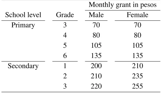
grant schedule is provided in Table 1.9

9_{The program also provided cash transfer and nutritional supplements for infants and small children that}

Table 1: PROGRESA monthly education grant schedule in 1998 Monthly grant in pesos School level Grade Male Female

Primary 3 70 70

4 80 80

5 105 105

6 135 135

Secondary 1 200 210

2 210 235

3 220 255

Source: Schultz (2004)

For the evaluation of the program, village- and household-level survey data was

col-lected in 506 randomly secol-lected villages. Moreover, a randomization of treatment villages

and control villages was performed. The beneficiary households in 324 treatment villages

started receiving the program transfers in 1998 and those in 182 control villages did at the

end of 1999. The survey data was collected in both treatment and control villages before

and after the implementation of the program. The baseline surveys were done in October

1997 and March 1998, and the three follow-up surveys were conducted in October 1998,

May 1999, and November 1999, all before the control villages started receiving the

pro-gram transfers. Every household in selected villages was surveyed; in the baseline surveys

there were 24,077 households (9,221 in the control villages and 14,856 in the treatment

villages). The household-level survey contains information about household members,

including their age, most recently completed school grade, school attendance,

employ-ment, and information about individual members’ wage income, household income from

other sources, household food consumption, and household expenditure on both food and

non-food items.

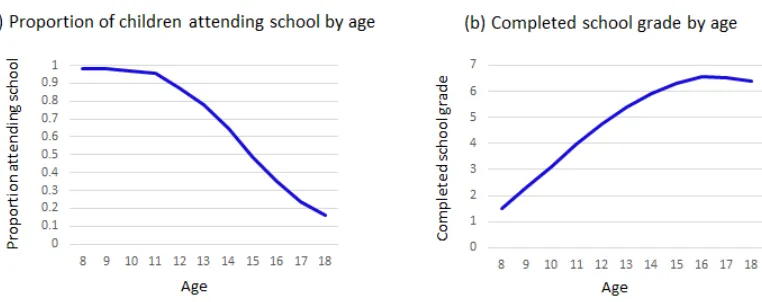
Figure 1: School enrollment rate and completed school grade by age

Source: PROGRESA data October 1998, May 1999, and November 1999. The sample is restricted to all control villages.

Table 2: Proportion of children making transitions into or out of school All Age≤12 Age>12 No transition into or out of school 0.72 0.80 0.43

One transition 0.18 0.12 0.38

Two transitions or more 0.11 0.08 0.20 Number of observations 16,981

Source: De Janvry et al. (2006). PROGRESA data over 7 semesters from November 1997-November 2000.

school for the entire semester. School enrollment is almost universal before age 12 and

starts to drop sharply around age 14. In control villages, the school enrollment rate

be-tween ages 16 and 18 during the data periods is around 30 percent, and the completed

grade of children at age 18 is less than 7th grade (Figure 1). School attendance is not only

low but also irregular. As shown in Table 2, 20 percent of children of the age of 12 and

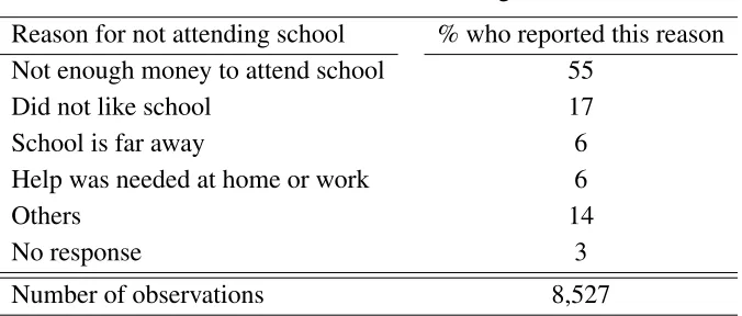
above make at least two transitions into and out of school. Table 3 shows that the most

frequently cited reason for absence is “not enough money”, which suggests that financial

constraint is important determinant of observed schooling outcomes in these villages.

Child labor is prevalent and a significant source of income in these villages. Child

Table 3: Reasons for not attending school

Reason for not attending school % who reported this reason Not enough money to attend school 55

Did not like school 17

School is far away 6

Help was needed at home or work 6

Others 14

No response 3

Number of observations 8,527

Source: PROGRESA data October 1998, May 1999, and November 1999. The sample is restricted to all control villages and children between the ages of 12 and 18.

wage reaches 35 percent by the age of 18 (Figure 2(a)). The contribution of children

(including zero wage) to household income increases with the age of the oldest child,

reaching 30 percent of total household income at the age of 18 (Figure 2(b)). In families

where a child works for a wage, the proportion of their contribution to household income

is 40 percent (Figure 2(c)).

In the data, only 1.2 percent of children between the ages of 12 and 18 were both

attending school and working. The assumption that the activity choices are mutually

exclusive does not seem to be very restrictive.10 Also, only 0.4 percent of the children

below age 12 worked.

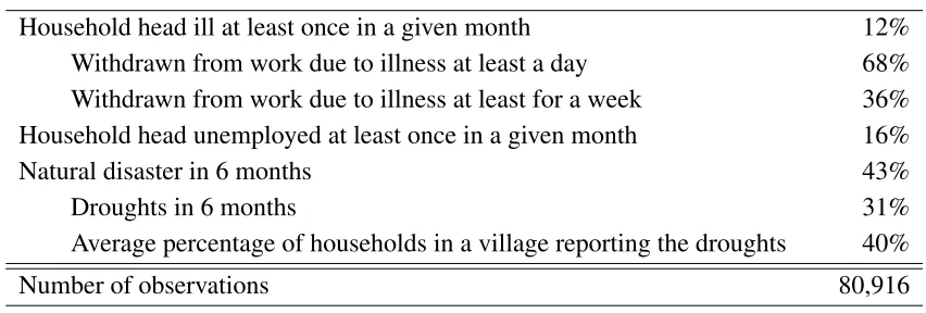
Table 4 shows the prevalence of shocks faced by households in PROGRESA villages.

In the data, 12 percent of households reported that their head had fallen ill at least once

within a given month, and almost 70 percent of them had to withdraw from work for one

or more days due to the illness. Also, 16 percent of households reported that their head

was unemployed at a certain point in a given month. Natural disasters such as droughts are

also common. 40 percent of households reported that they had experienced a drought at

10_{When children are both attending school and working, I treat them as attending school regardless of}

Figure 2: Child labor in PROGRESA villages

Table 4: Percentage of households having experienced various shocks

Household head ill at least once in a given month 12% Withdrawn from work due to illness at least a day 68% Withdrawn from work due to illness at least for a week 36% Household head unemployed at least once in a given month 16%

Natural disaster in 6 months 43%

Droughts in 6 months 31%

Average percentage of households in a village reporting the droughts 40%

Number of observations 80,916

Source: PROGRESA data October 1998, May 1999, and November 1999. All villages.

least once within the past 6 months. Droughts are regarded as a community-wide shock;

however, not all households in a village reported the experience of the same shock. In

a given village, on average, 4 out of 10 households report that they had experienced a

drought whereas 6 out of 10 households reported that they had not experienced any during

the same periods. Reported damage also varied across households in each given village,

suggesting that there is a room for risk sharing among households in a village even in

times of natural disaster.

There is evidence that households exchange informal transfers and rely on informal

sources to borrow money in PROGRESA villages. As shown in Table 5, 10 percent of

households reported some form of support received from or given to other households

within a single month.11 The average amount of support was 475 pesos, which is a

sub-stantial amount considering that the average monthly household expenditure is 1,071

pe-sos in these villages. Also, more than 60 percent of reported credit (in frequency, not

in the amount of money) was from informal sources such as relatives, neighbors, and

11_{10 percent is arguably not large enough to support a model assumption that every household participates}

Table 5: Informal financial activities in PROGRESA villages Giving or receiving support from other households

Percentage of households reported the activity 10% Average amount of the support 475 pesos Borrowing or credit

Percentage of households reported the activity 2% Percentage of credit from relatives/neighbors/friends 62%

Number of observations 26,972

Source: PROGRESA data October 1998, May 1999, and November 1999. Average amount of the support is reported in nominal Mexican peso.

friends.

In addition, the data on income from other sources such as sales of a household

mem-ber’s service, crop production, livestock sales, government program transfers other than

PROGRESA (such as pensions), rent, and any interest from savings were also available.

Household income variable was constructed as the sum of all members’ wage income and

income from other sources. Parental income is obtained by subtracting the sum of the

wage income of children from household income.

The survey also contains detailed information about the quantity and the value of

household food consumption, non-food expenditures, and income from various sources.

The consumption variables are available in the October 1998, May 1999, and November

1999 waves, but not in the baseline surveys; thus, in my analysis, only the later three

waves are used. I convert the household income and consumption to the adult-equivalent

per-capita level adjusted by the economies of scale. The adult equivalent weights are

based on the calculation of Di Maro (2004).12 See Appendix C for details about how the

income and consumption and variables are constructed.

12_{Di Maro (2004) assigns 1 on adult members above age 18 and 0.73 on members of age 18 and below.}

Then I further adjust the adult equivalent size of the households for the economies of scale by taking a square root. For example, in a household that has two adults who are age 40 and three children who are age 10,

In the estimation, I use the 11 largest control villages, which have more than 100

households each. I restrict the sample to large control villages for two reasons. First, I

use large villages because the model assumes a continuum of households, which is better

approximated by large villages. Second, I use control villages because the model solution

algorithm requires stationarity of the economy. In treatment villages, the village economy

may be on a transition path to a different steady state than in the control villages, due to

the introduction of the cash transfer program. There are 1,433 households in the selected

sample. Also, when I map the model to the data, I only track the information about

the oldest child of each household. For example, the model outcomes such as school

attendance and the accepted wage of a 12-year-old-child are compared to the observed

outcomes of the households whose oldest child is 12 years of age in the data.13 Table 6

provides the summary statistics of the selected sample. The school enrollment rate and

the fraction of children working for a wage by age is based on the oldest child. When

constructing moments in the estimation, income is deflated so that the aggregate income

level is the same as the aggregate consumption level.14

13_{In PROGRESA villages, the birth order does not seem to affect the school attendance decision much}

as the coefficient of the birth order variable in the probit regression of the school enrollment was close to zero and not significant at conventional level. The sample used in the analysis was comprised of all children between ages 6 and 18 in both the treatment and control villages (about 48,000 children in total). Other controls were age, gender, parental education, completed grade, and village-fixed effect. The most important determinant was the age of a child.

14_{The aggregate consumption-to-income ratios in each village are 0.58, 0.68, 0.96, 0.56, 0.66, 0.67, 0.77,}

Table 6: Summary statistics

mean (s.d.) Completed school grade

mothers 3.18 (2.69)

fathers 3.81 (2.56)

children at age 18 7.42 (2.37) School enrollment rate

6≤age≤11 .98 (.13)

12≤age≤15 .77 (.42)

16≤age≤18 .36 (.48)

Fraction of children working for wage

12≤age≤15 .06 (.24)

16≤age≤18 .31 (.46)

Children’s wage income 1,179.24 (1,232.13) Household income 2,478.75 (2,978.39)

Number of observations 4,152

4

Estimation

I use the method of simulated moments to estimate the model parameters.15 This

estima-tion method finds a set of parameter values that minimizes the weighted distance between

the aggregate moments constructed with the data and that of the simulated outcomes of the

model. The weights are given by the inverse of estimated variances of the data moments

following Lee and Wolpin (2010).

The simulated moments are generated from the computed stationary distribution for

a given set of parameters. I use the observed completed school grade of mothers and

the estimated type-probability process to determine the type of parents of each

house-hold. Given the parental type, the age and completed school grade of each child is drawn

from the stationary distribution. I assume that the state of the economy when the

par-ents’ schooling investment was made is different from the current steady state and that

the parental schooling distribution and the parental type distribution are exogenous to

the model. I also assume that the new households entering the economy have the same

schooling distribution as the mothers in the sample. Thus, the parental schooling

distribu-tion and the resulting parental type distribudistribu-tion are constant over time. Given the parental

15_{Parameters in the model are identified by the combination of functional forms, distributional}

assump-tions, and exclusion restrictions.µpin the parental and household income processes for high-income type

are normalized to be zero. Although the parameters in the parental and household income processes are identified outside the model, estimating the income process jointly with other model parameters makes the estimation more efficient. This is because the parameters in the income process determine the return from schooling, and thus they affect other parameters that govern child activity choices. I fix the subjective

dis-count factorδ at a conventional level of 0.95 because with a constant relative risk aversion (CRRA) utility

function it is not obvious how to separately identify the risk aversion and time discounting parameters.

Grade-completion probability for grades 7-12,πgr(dtschool,dtschool−1 )are not estimated but imputed based on

the fraction of children completing one school grade given their observed enrollment status. The computed

grade-completion probability for grades 7-12 is given byπgr(1,1) =0.8,πgr(1,0) =πgr(0,1) =0.25, and

πgr(0,0) =0.1. Grade-completion probability for children below age 12 (or between grades 1-6),π_gr12(X,k),

for each(X,k)are estimated whereXis a school grade in which a child is enrolled andkis a parental type.

Althoughπgr(dtschool,dtschool−1 )is independent of parental type, the proportion of children who complete a

school grade each year can differ across different parental types becausedschool

t is a choice and is affected

by parental type. Demographic transition probabilitiesπb,πm, andπdare also imputed based on the

type, the age and the completed school grade of a child, and a set of shocks, an efficient

allocation is computed by solving the agent’s problem. Then, the simulated moments are

constructed as an average over the outcomes which are associated with many different

sets of shocks.

Target moments used in the estimation are listed below. A “grown-up child” refers to

a child whose age is above 18.

1. Income process

(a) Mean parental income by village, excluding households with a grown-up child

(b) Mean household income by village (households with a grown-up child only)

(c) Standard deviation of mean-differenced log parental income by village,

ex-cluding households with a grown-up child

(d) Standard deviation of mean-differenced log household income by village

(house-holds with a grown-up child only)

(e) Mean parental income by the completed grade of mothers, excluding

house-holds with a grown-up child

(f) Mean parental income by the completed grade of mothers (households with a

grown-up child only)

(g) Mean household income by the completed grade of children (households with

a grown-up child only)

(h) Standard deviation of log parental income by the completed grade of mothers,

excluding households with a grown-up child only

(i) Standard deviation of log household income by the completed grade of

2. Child wage process

(a) Mean accepted wage by age, from ages 12 to 18

(b) Mean accepted wage by parental income quartile

(c) Mean accepted wage by the completed grade of mothers.

3. Child activity choice

(a) Proportion of children attending school and working by age, from age 12 to

age 18

(b) Proportion of children staying home, attending school, and working between

ages 12 and 16 by parental income quartile

(c) Proportion of children attending in each of the 5th, 6th, 8th, and 9th grades

(d) Proportion of children attending school in the spring but who were not

en-rolled in the previous fall

(e) Proportion of children attending school in the fall but were not enrolled in the

previous spring

(f) Proportion of children attending school by years behind the standard grade

level at each age

(g) Mean parental income of households with a child attending middle school

(grades 7 to 9)

(h) Mean parental income of households whose child is eligible to attend middle

school but stays home

(i) Mean parental income of households whose child attends high school (grades

(j) Mean parental income of households whose child is eligible for high school

but stays home.

4. School grade completion16

(a) Proportion of 12-year-old children who completed no grade, 1st grade, 2nd

grade, ..., 6th grade by the completed school grade of their mothers.

5. Consumption

(a) Mean consumption by the completed grade of mothers

(b) Mean consumption by the completed grade of child (households with a

grown-up child only)

(c) Mean consumption by parental income quartile

(d) Correlation of mean-differenced household income and consumption over time.

4.1

Parameter estimates

The estimated parameters are shown in Table 7-Table 10.17 I discuss the parameter

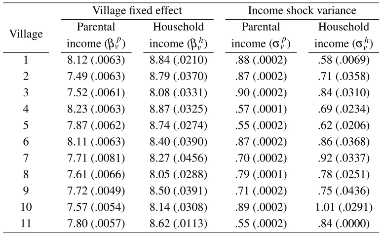
Table 7: Parameter estimates: income process

Village fixed effect Income shock variance

Village Parental Household Parental Household income (βvp) income (βvh) income (σ

p

v) income (σvh)

1 8.12 (.0063) 8.84 (.0210) .88 (.0002) .58 (.0069) 2 7.49 (.0063) 8.79 (.0370) .87 (.0002) .71 (.0358) 3 7.52 (.0061) 8.08 (.0331) .90 (.0002) .84 (.0310) 4 8.23 (.0063) 8.87 (.0325) .57 (.0001) .69 (.0234) 5 7.87 (.0062) 8.74 (.0274) .55 (.0002) .62 (.0206) 6 8.11 (.0063) 8.40 (.0390) .87 (.0002) .86 (.0368) 7 7.71 (.0081) 8.27 (.0456) .70 (.0002) .92 (.0337) 8 7.61 (.0066) 8.05 (.0288) .79 (.0001) .78 (.0251) 9 7.72 (.0049) 8.50 (.0391) .71 (.0002) .75 (.0436) 10 7.57 (.0054) 8.14 (.0308) .89 (.0002) 1.01 (.0291) 11 7.80 (.0057) 8.62 (.0113) .55 (.0002) .84 (.0000)

Notes: Standard errors are in parentheses.

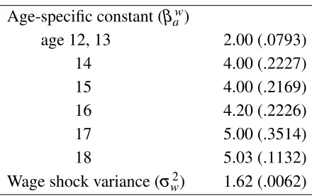
4.1.1 Income, wage, and type process parameters

Table 7-Table 9 provide parameter estimates for parental income, child wage, household

income, and type process parameters. As shown in Table 7, the mean and the variance of

parental and household income vary significantly across villages. In all villages,

house-hold income with a grown-up child is larger than that of other househouse-holds. Table 8

pro-vides parameter estimates for the child wage process. Mean wage offers for children

substantially increase with the child’s age, implying a higher opportunity cost of

attend-ing school for older children. Table 9 provides type process parameter estimates. The

16_{The current estimation on which the results reported in the paper are based does not incorporate the}

moments related to school grade completion. School grade completion probabilitiesπ_gr12(X,ptype) for

X=0, ...,6 andptype=low,highare calibrated. The results of the full estimation are forthcoming. The

calibrated values are given by the following. The numbers may not sum up to 1 because they are rounded:

ptype\X 0 1 2 3 4 5 6

low 0.03 0.01 0.05 0.12 0.27 0.28 0.13 high 0.08 0.01 0.01 0.05 0.08 0.31 0.47

Table 8: Parameter estimates: child wage process Age-specific constant (β_aw)

age 12, 13 2.00 (.0793)

14 4.00 (.2227)

15 4.00 (.2169)

16 4.20 (.2226)

17 5.00 (.3514)

18 5.03 (.1132)

Wage shock variance (σ_w2) 1.62 (.0062)

Notes: Standard errors are in parentheses.

estimated type component in income process, µp, is -0.9 for the low-income type,

trans-lating to a mean income that is 41 percent of high-income-type ones.18 This is compatible

with the observed difference in mean incomes of poor (CCT beneficiaries) and non-poor

households in the data.19 The estimated parameters in the type probability process predict

that the probability of being a high-income-type child when no grade is completed is 0.25

and that completing the 6th, 9th, and 12th grades increases this probability to 0.48, 0.56,

and 0.66 respectively. Combined with the estimated µp, the estimated type probability

process predicts that, compared to those who did not finish any school grade, the expected

mean household income is 24, 33, and 43 percent higher when a child completes 6th, 9th,

and 12th grades.20 The type components of parents and children enter multiplicatively in

18_{This calculation is done by:}

Realized income of low-income type

Realized income of high-income type =

eβv+µp+εp

eβv+εp ==exp(−0.9)'0.41

19_{In the sample used in the estimation, the observed mean of per adult-equivalent household income of}

the beneficiary households for 6 months is 1835.68 pesos and that of the non-beneficiary households is 3022.26 pesos.

20_{The relative size of income is obtained by the following calculations:}

(A) Mean income of those who did not complete any school grade = 0.75eβv−µp+0.5σvp_+0.25eβv+0.5σvp

(B) Mean income of those who completed 6th grade =0.52eβv−µp+0.5σvp_+0.48eβv+0.5σvp

Table 9: Parameter estimates: type process Unobserved type component in income process

Constant term for low-income type (µ) -.90 (.0058)

Type probability process (probability of being high-income type) When completed grade is observed

Constant (γ0) -1.00 (.0021)

Coefficient of completed school grade

For grade between 1 and 6 (γX,primary) .10 (.0143)

For grade above 6 (γX,secondary) .08 (.0183)

Coefficient of completing primary school (γ6) .30 (.0595)

Coefficient of completing middle school (γ9) .12 (.0132)

Coefficient of completing high school (γ12) .17 (.0123)

When completed grade is not observed

Constant (γX0) .80 (.0130)

Notes: Standard errors are in parentheses.

the household income process, and households with high-income type parents have larger

return from schooling.

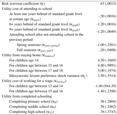
4.1.2 Preference Parameters

Preference parameter estimates are provided in Table 10. The estimated risk aversion

coefficient is 0.63. This is within the range of the values which were found in other

studies that structurally estimate limited-commitment risk-sharing models using

village-level data in developing countries.21

The estimated parameters for utilities from completing primary, middle, and high

school are 0.30, 0.50, and 0.75 respectively. To provide an idea of how large these

num-21_{Other papers that structurally estimate a limited-commitment risk-sharing model by using data from}

Table 10: Parameter estimates: preference

Risk aversion coefficient (η) .63 (.0015)

Utility cost of attending to school

At least one years behind of standard grade level

-.50 (.0016) at certain age (κgap1)

6+ years behind of standard grade level (κgap6) -1.20 (.0016)

9+ years behind of standard grade level (κgap9)

-1.20 (.0049) Attending school after not attending school in the

previous period

Spring semester (κprev,spring) -1.00 (.2561)

Fall semester (κ_prev,f all) -.20 (.0408)

Utility from staying home(κhome,a)

For children age 14 4.50 (.1669)

For children age between 15 and 16 4.80 (.9891) For children age between 17 and 18 5.00 (.1974) Idiosyncratic leisure preference shock variance (σ_ξ) 3.50 (.5514)

Utility cost of working for a wage(κwork,a)

For children age between 12 and 14 -1.40 (944.29) For children age between 15 and 16 -1.40 (.2398) Utility from completed schooling

Completing primary school (κ6) .36 (.2804)

Completing middle school (κ9) .56 (.2462)

Completing high school (κ12) .76 (.3743)

Notes: Standard errors are in parentheses.

bers are I convert them into consumption-equivalent terms given a reference consumption

level of 2,634.46 pesos, which is the estimated mean consumption level in the economy.

The utilities from completing schools are translated into 183.42, 210.57, and 259.24

addi-tional pesos of consumption respectively, compared to the households of which the child

did not finish primary school.22

The estimated parameters for the leisure value of a child are translated into 100.34

22_{The consumption-equivalent values were obtained by the following way. Suppose that a household has}

household consumption of 2,634.46 pesos (which is the average amount of consumption in the villages) and