The Solution of Advection Diffusion Equation by The Finite Elements Method

(1)

The Solution of Advection Diffusion Equation by the

Finite Elements Method

Hasan BULUT

1

, Tolga AKTURK

1

and Yusuf UCAR

2

1

Department of Mathematics, Firat University, 23119, Elazig -TURKEY

2

Department of Mathematics, Inonu University, 44280, Malatya-TURKEY

[email protected], [email protected] , [email protected]

Abstract

--

In this study, we have tried to find the numerical solutions of Advection diffusion equation (ADE) by Galerkin method (GM), Adomian decomposition method (ADM) and Homotopy perturbation method (HPM); and then, we have formed a table that contains numerical results for this equati on by drawing the graphic of that equation using Origin 8. Finally, we have made a comparison between GM, ADM and HPM for ADE.

Index Term

--

Linear Advection diffusion equation, Homotopy perturbation method, Galerkin method, Adomian decomposition method.

1. INTRODUCTION

ADE describes [12,13,21,26] many quantities such as mass, heat, energy, velocity, vorticity, etc. The solutions of this equation model some of the phenomena such as the heat transfer in a draining film, water transfer in soils, spread of pollutants in rivers and streams, contaminant dispersion in shallow lakes, flow in porous media, dispersion of dissolved salts in groundwater, thermal pollution in river systems, etc. The slow progress has been made towards the analytical solutions of ADE when initial and boundary conditions are complicated. Besides many of the analytical solutions have not much easy use. So a great deal of efforts have been given on developing the efficient and stable numerical techniques. Various numerical techniques have been proposed to illuminate physical phenomena described by ADE in many disciplines. The difficulties arising in numerical solutions of ADE result from the dominant advection, which is for relatively high peclect number.

2. ANALYSIS OF THE METHODS

2.1 Galerkin Method (GM)

For the choice of weight function



_iequal to the

approximation function



_i, the weighted-residual method is

better known as Galerkin method [2,4,14,18,20,23,]. The

algebraic equations of the Galerkin approximation are

1

N

ij i i

j

A



f





(2.1.1)

where

 

ij j j

A



A



dxdy







and

 



0



i j

f



f

A



dxdy









. (2.1.2)

We note that

A

_ij is not symmetric.

2.2 Homotopy Perturbation Method (HPM)

To illustrate the basic ideas of this method, we consider the following nonlinear differential equation,

 

0,

A u



f r



r



, (2.2.1)

with the boundary conditions



,

/



0,

,

B u u

  

n

r



(2.2.2)

where

A

is a general differential operator,

B

is a boundary operator,

f r

 

is a known analytical function and



is the

boundary of the domain



. Generally speaking, the operator

A

can be divided into two parts, namely

L

and

N

, where

L

is linear, while

N

is nonlinear. Eq.(2.2.1) can be rewritten as following

 

( )

 

0. L u



N u



f r



(2.2.3)

By the homotopy technique, we construct a homotopy

 

,

:

 

0,1

V r p





R

which satisfies;

0

( , )

(1

)[ ( )

( )]

[ ( )

( )]

0 H v p

 

p L v



L u



p A v



f r



(2.2.4) or

     

,

0

 

0

   

0,

H v p



L v



L u



pL u



p N v



_



f r



_



(2.2.5)

where

p



 

0,1

is an embedding parameter,

u

₀ is an initial approximation of Eq.(2.2.1). Obviously, from Eq.(2.2.4) and Eq.(2.2.5), we will have

0

( , 0)

( )

0 H v



L v



L u



(2)

and

( ,1)

( )

0 H v



A v



f r



(2.2.7)

the changing process of p from zero to unity is just that of

( , )

V r p

from

u r

₀

( )

to

u r

( )

.

In topology, this is called deformation, and

L v

( )



L u

( )

₀

and

A v

( )



f r

( )

are called homotopy. According to the HPM, we can first use the embedding parameter p as a "small parameter", and assume that the solution of Eq.(2.2.4) and Eq.(2.2.5) can be written as a power series in

p

;

2 3

0 1 2 3

.

V

 

V

pV



p V



p V



(2.2.8)

Setting

p



1

results in the approximate solution of

Eq.(2.2.1) and Eq.(2.2.2);

0 1 2 3

1

lim

p

u

V





   

(2.2.9)

The convergence of series in Eq.(2.2.9) has been proved by He in his paper [7]. This technique can have full advantage of the traditional perturbation techniques. The series in Eq.(2.2.9) is convergent rate depends on the non -linear operator

A v

( )

(the following opinions are suggested by He [7]:

(1) The second derivative of

N v

( )

with respect to

v

must be small because the parameter may be relatively large, i.e.,

p



1

.

(2) The norm of

L

1

(



N

/



v

)

must be smaller than one so that the series converges.

3. APPLICATION OF METHODS TO ADE 3.1 Application of GM

In this section,

0

t x xx

u

 

u



,

0

<

x

< 1 , t > 1. (3.1.1)

We consider ADE by the beginning condition of

 

₅₀2

, 0

x

,

1 200

u x



e



s

 

vt

(3.1.2) [21] (v: emission speed, s: emission space). An exact

solution of this problem is

 

1 



2

,

exp

50 x t

.

U x t

s



_







_





_





Although there are approximate solutions of this problem, the necessary boundary conditions were taken from the exact solution of the problem.

In this section, the approximate results of Eq.(3.1.1) were obtained by GM using Quadratic B-spline functions. The approach solution that corresponds to the exact solution of the

problem

U x t

 

,

in terms of B-spline functions

 

   

1

,

N

N j j

j

U

x t



t Q x







(3.1.3)

will be observed. Here,



_jare time dependent unknown

parameters. To Quadratic B-spline functions, if

 

a b

,

interval is

a



x

₀<

x

₁<

x

₂< <

x

_N



b

by separating parts

h



x

_m_₁



x

_m lengths in



x x

_m

,

_m_₁



interval.

When the transition



 

x

_m ,

0  



h

is used, the following B-splines

2 2

1 2

2

m

Q

h



 



(3.1.4)

2

1

1 2

2

m

Q

h

 



 



(3.1.5)

2 1 2

m

Q

h







(3.1.6)

are obtained. On



x x

m

,

m1



element, all other splines are

zero, in terms of quadric base functions,

U

_N

 

x t

,

approach is written as

 

1

   

1

,

m

N j j

j m

U

x t



t Q x



 





(3.1.7)

If Eq.(3.1.4) – Eq.(3.1.6) Quadratic B-spline functions and

(3)

pointal values of primary derivations to

U

_m and x according to



_j parameters are written as;

 





1 ' 1

2

m m m m

U

x

U

x

h



 









where

m



0,1,

,

N



1,

N

Now, to form the nominal integral form of ADE, if it is multiplied with nominal function and then its integral is taken from the space, it is obtained as,





1 0

0

t x xx

U

dx











(3.1.8)

The nominal integral form on finite element



x x

_m

,

_m_₁



, it is obtained as





1

0

m m x

t x xx

x

U

dx











(3.1.9)

Eq.(3.1. 9) nominal integral form is arranged as following,

1 1 1

0

m m m

x x x

t x xx

x x x

U dx



  









(3.1.10)

When partial integration is applied to 1 m m x xx x

U dx







term,





1 1 m m m m x x

t x x x _{x x}

x

U

dx

U









(3.1.11)

is obtained. According to GM, in Eq.(3.1.11) equation,

i

Q





is selected and if

U

_N approximate solution is taken instead of

U

, in terms of

i

 

m

1, ,

m m



1

1 1

' ' ' '

0

1 0 0 0 1

j i j j

h h h

m m _h

j

i j i j j i

j m j m

Q Q



Q Q



Q Q



Q Q

      























(3.1.12)

is obtained . Superscripts prime and dot denote derivative with respect to space and time, respectively. From this, if

0

h e

ij i j

A





Q Q d



'

0

h e

ij i j

B





Q Q d



' '

0

h e

ij i j

C





Q Q d



'

0

h e

ij i j

D



Q Q

Eq. (3.1.12) equation system is written in matrix form as,

e e e e

A



B



C



D









(3.1.13)

From this, the matrixes of

6

13

1 13 54 13

30

1

13

6

e

h

A











_

_









3

2

1

8

0

8

6

1 2 3

e

B













_



_











2

1

2

1

2

1

3

1

2

e

C

h













_



_











1 1 0

2

1 2 1

0 1 1

e

D

h













_



_











are obtained. The general lines of

A B C D

, , ,

that are obtained by the unifying of

A B C

e

,

e

,

e and

D

e element matrixes are as follows,

















:

1, 26, 66, 26,1

30

1 :

1, 10, 0,10,1

6

2 :

1, 2, 6, 2, 1

3

2 :

0, 0, 0, 0, 0

(4)

By using the unified matrixes in (3.1.13),

A

 



B C

D



0





 



(3.1.14)

is obtained. In Eq.(3.1.14) equation, instead of





, if

1

n n

t













forward finite difference approach below is written and instead of



, if

1

2

n n







Crank-Nicolson finite difference approach is written,





1





2

n n

t

A



B C

D





A



B C

D





_

_{ }



_



_

_{ }



















(3.1.15)

equation system is found.

To calculate



_mn parameters, firstly



0 initial vector should

be calculated. Vector



0 will be calculated by using

 

, 0

U x

initial and boundary conditions given with the

problems.

To calculate the initial parameters,

U

_Napproach is written as follows,

 

0

1

, 0

N

N j j

j

U

x



Q







Here,



0_j is the parameters that will be determined. So, by using

 

, 0

 

, 0 ,

0,

,

N j

U

x



U x

j



N

values,



0_j parameters





















0 1 0

1 0 1

2 1 2

1 2 1

1

, 0

N N N

U x



 





  











 









are obtained. In this system,

N



1

equation

N



2

unknown

exist. As a complementery condition, if

  



'

1

2

j j j

U x

h

 







derived boundary condition is used,

 





' '

0 0 0 1

2 U x

U

h

 







is obtained. If parameter



_₁is abolished, a system consisting

of

N



1

unknown

N



1

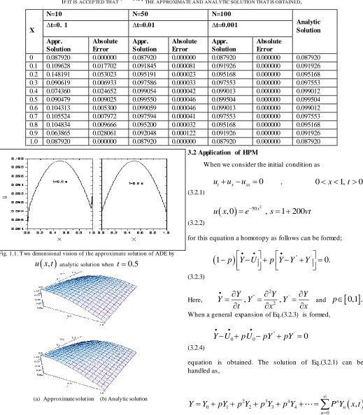
numbered is obtained. By this data

(5)

TABLE 1.1.

IF IT IS ACCEP TED THAT

t



0.5,

THE AP P ROXIMATE AND ANALYTIC SOLUTION THAT IS OBTAINED,

Fig. 1.1. T wo dimensional vision of the approximate solution of ADE by

 

,

u x t

analytic solution when

t



0.5

(a) Approximate solution (b) Analytic solution

Fig. 1.2. T hree dimensional vision of the approximate solution of ADE by

 

,

u x t

t



0.5

3.2 Application of HPM

When we consider the initial condition as

0

t x xx

u

 

u



,

0  

x

1,

t



0

(3.2.1)

 

₅₀2

, 0

x

,

1 200

u x



e



s

 

vt

(3.2.2)

for this equation a homotopy as follows can be formed;





'' '

1 p

Y U

p Y Y

Y

0.

  











_



_



_





_











(3.2.3)

Here,

2

'' '

2

,

Y

t

x









and

p



 

0,1 .

When a general expansion of Eq.(3.2.3) is formed,

'' '

0 0

0 Y U

pU

pY

  











(3.2.4)

equation is obtained. The solution of Eq.(3.2.1) can be handled as,

 

2 3 4

0 1 2 3 4

0

,

n n n

Y

pY

p Y

P Y

x t





 







(3.2.5) X

N=10 N=50 N=100

Analytic Solution

∆t=0. 1 ∆t=0.01 ∆t=0.001

Appr. Solution

Absolute Error

0 0.087920 0.000000 0.087920 0.000000 0.087920 0.000000 0.087920

0.1 0.109628 0.017702 0.091845 0.000081 0.091926 0.000000 0.091926

0.2 0.148191 0.053023 0.095191 0.000023 0.095168 0.000000 0.095168

0.3 0.090619 0.006933 0.097586 0.000033 0.097553 0.000000 0.097553

0.4 0.074360 0.024652 0.099054 0.000042 0.099013 0.000000 0.099012

0.5 0.090479 0.009025 0.099550 0.000046 0.099504 0.000000 0.099504

0.6 0.104313 0.005300 0.099059 0.000046 0.099013 0.000000 0.099012

0.7 0.105524 0.007972 0.097594 0.000041 0.097553 0.000000 0.097553

0.8 0.104834 0.009666 0.095200 0.000032 0.095168 0.000000 0.095168

0.9 0.063865 0.028061 0.092048 0.000122 0.091926 0.000000 0.091926

(6)

 

'' '' '' 2 '' 3 '' 4 '' ''

0 1 2 3 4

0

,

n n n

Y

pY

p Y

P Y

x t











(3.2.6)

 

2 3 4

0 1 2 3 4

0

,

n n n

Y

pY

p Y

P Y

x t

        









(3.2.7)

 

' ' ' 2 ' 3 ' 4 ' '

0 1 2 3 4

0

,

n n n

Y

pY

p Y

P Y

x t











(3.2.8)

By writing Eq.(3.2.5) – Eq.(3.2.8) in Eq.(3.2.4),

'' '

0 0

0 Y U

pU

pY

  











2 3 4 '' '' 2 '' 3 '' 4 ''

0 1 2 3 4 0 0 ₀ ₁ ₂ ₃ ₄

' ' 2 ' 3 ' 4 '

0 1 2 3 4

0 Y

pY p Y

p Y

U

pU

p Y

pY

p Y

pY

p Y

      



_



_{ }

_

_

_

_



















_



_



2 3 4 '' '' 2 '' 3 '' 4 ''

0 1 2 3 4 0 0 ₀ ₁ ₂ ₃ ₄

' ' 2 ' 3 ' 4 '

0 1 2 3 4

0 Y

pY

p Y

p Y U

pU

pY

p Y

pY

p Y

      



 







are obtained. If this equation is re-formed according to the

terms in the same order of p,

0

0 0

:

0 p

Y

U

 





(3.2.9)

p Y

1

:

1

U

0

Y

₀''

Y

₀'

0

 









(3.2.10)

2 '' '

2 ₁ ₁

:

0 p

Y









(3.2.11)

p

3

:

Y

3

Y

₂''

Y

₂'

0









(3.2.12)

4 '' '

4 ₃ ₃

:

0 p

Y









(3.2.13)

is obtained. While the solution of Eq.(3.2.9) –Eq. (3.2.13) are as follows,

2

0

0 0 0 0

50 0

:

0

x

p

Y

U

Y

U

Y

e

   



 









2



_

_

1 '' ' '' '

1 0 ₀ ₀ 1 0 ₀ ₀

'' ' 0

1 0 0

0

50 ₂

1

:

0

100

1

100

t

x

p Y

U

Y

U

Y

U

Y

dt

Y

e

t

x

     







 

 









 

_







_





 

  



(3.2.15)

 

2

_

_

2 '' ' '' '

2 ₁ ₁ 2 ₁ ₁

'' '

2 1 1

0

50

'' ' 2 2 3 4

1 1 2

:

0

50 299 600

59900

20000

1000000

t

x

p Y Y

Y

Y dt

Y

Y Y

e

t

x

  

     





 

_



_



















(3.2.16)





_

_





_

_

2 2

3 '' ' '' '

3 ₂ ₂ 3 ₂ ₂

'' '

3 2 2

0

50 ₃ ₂ ₃

3

50 ₃ ₄ ₅ ₆

:

0 5000

1491 4497

448200

299900

3 5000

14970000

3000000

10000000

3

t

x

p Y

Y

dt

Y

e

t

x

e

t

x

   

   









 

_



_

 















(3.2.17)





_

_





_

_





_

_

2 2 2

4 '' ' '' '

4 ₃ ₃ 4 ₃ ₃

'' '

4 3 3

0

50 ₄ ₃ ₂

4

50 ₄ ₅ ₃ ₄ ₄ ₆ ₅

50 ₄ ₈ ₆ ₁₀ ₇ ₁₂ ₈

:

0 1250

1041003 4194.10

4173000600

(3.2.18)

3 1250

4196.10

2091001.10

8396.10

3 1250

2794.10

4.10

10

3

t

x

p Y

Y

Y dt

Y

e

t

x

e

t

x

e

t

x

    

   

 





 

_



_

 











(7)

 

















_

_





_

_





2 2

2

2 2

50 50 ₂

0 1 2 3 4

1

50 ₂ ₂ ₄ ₃ ₆ ₄

50 ₂ ₂ ₄ ₃ ₆ ₄ 50 ₃

2 3 4 4 6 5

,

lim

100

1

100 299 600

59900

210

10 5000

299 600

59900

210

10

3 1491 4497

448200

299900

149710

3.10

10

x x

p

x

x x

U x t

Y

e

t

x

e

t

x

e

t

x

e

t

x

 





 



    





  























_

_





_

_

2

8 6

50 ₄ ₃ ₂ ₅ ₃

50

4 4 4 6 5 8 6 10 7 12 8

1250

1041003 4194.10

4173000600

4196.10

3 1250

2091001.10

8396.10

2794.10

4.10

10

3

x

e

t

x

e

t

x













is obtained . So, the closed form of analytic solution of Eq.(3.2.1) is,

 

1 



2

,

exp

50 x t

.

u x t

s



_







_





_





According to the obtained solutions, 2D-3D graphics of given

ADE by HPM when

t



0.5

are given below.

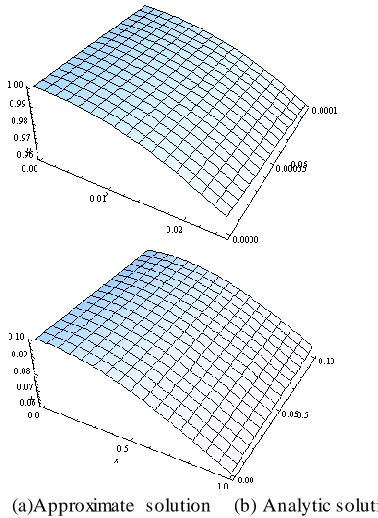
(a)Approximatesolution (b) Analytic solution

Fig. 1.5. (HPM) T wo dimensional vision of the approximate solution and

analytic solution of ADE by

u x t

 

,

t



0.5

(a)Approximate solution (b) Analytic solution

Fig. 1.6. (HPM) three dimensional vision of the approximate solution and

u x t

 

,

t



0.5

3.3 Application of ADM

Consider ADE given with Eq.(3.1.1) and Eq.(3.1.2) equations. This equation can be written as follows in the form of anoperator,

0

t x xx

L



L u



L u



(8)

Here,

L

_t

t







,

L

x







and

2 2 xx

L

x







. Here,

1

t

L

 is an

integral operator and 1

 

0

.

t

L







dt

.

If

L

_t1 is applied to the both sides of Eq.(3.3.1),

 





1 1

t t t x xx

L



L u

 

L



L u L u



(3.3.2)

is obtained. So,





1

( , )

( , 0)

_t _x _xx

u x t



u x



L



L u L u



(3.3.3)

is obtained. For Eq.(3.3.3) , a recurrence connection can be written as follows,

 

2 50 0 1 0

, 0

,

1 200 ,

,

0,

,

x

t

k x k xx k

u x

u

e

s

vt

k

u

x t

L u

x t

L u

x t

dt

 



_

_{ }







 

















(3.3.4)

From the Eq.(3.3.4) recurrence connection that is obtained,





 





2

1

1 0 0 0 0

0

50 2

,

100

1

100

t

t x xx x xx

x

u

L

L u

x t

L u

x t

dt

e

t

x

 

 



 



_





_



  







 





2 1

2 1 1 1 1

0

50 2 2 4 3 6 4

,

50 299 600

59900

2.10 .

10

t

t x xx x xx

x

u

L

L u

L u x t

dt

e

t

x

 

 



 



_





_













 





2 1

3 2 2 2 2

0

50 3 2 3 4 4 6 5 8 6

,

5000

1491 4497

448200

299900

1497.10

3.10

10

3

t

t x xx x xx

x

u

L

L u

x t

L u

x t

dt

e

t

x

 

 



 



_





_

















 









2 2 1

4 3 3 3 3

0

50 4 2 5 3 4 4

50 4 6 5 8 6 10 7 12 8

,

1250

1041003 419000

417300600

4196.10

2091001.10 .

3 1250

8396.10 .

2794.10

4.10

10

3

t

t x xx x xx

x

u

L

L u

x t

L u

x t

dt

e

t

x

e

t

x

  

 



 



_





_













The first four terms of decomposition series are obtained.

When the obtained terms

u u u u u

₀

, ,

₁ ₂

,

₃

,

₄ are written in Eq.(2.3.6), the approximate solution of Eq.(3.3.1) ADE is,

 





2 2 2

2

0 1 2 3 4

0

2

50 50 2 50 2

4 3 6 4 2

50 3

3 4 4 6 5 8 6

,

299 600

59900

100

1

100

50 2.10 .

10 1491 4497

448200

5000

3 299900

1497.10

3.10

10

n n

x x x

x

u x t

u

x t

u

x

e

t

x

e

t

x

e

t

x

(9)

can be obtained as. So closed form analytical solution of the Eq.(3.1.1)

 

1 



2

,

exp

50 x t

.

u x t

s



_







_





_





According to the obtained solutions, 2D-3D graphics of given

ADE by ADM when

t



0.5

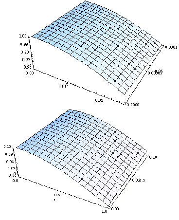
are given below.

(a) Approximate solution (b) Analytic Solution

Fig. 1.9. (ADM) T wo dimensional vision of the approximate solution and

u x t

 

,

t



0.5

(a) Approximate solution (b) Analytic solution

Fig. 1.10. (HPM) Three dimensional vision of the approximate solution and

u x t

 

,

t



0.5

4. CONCLUSION

In this study, GM, HPM and ADM have been applied successfully to ADE. It is seen that when the approximate

solution of ADE is formed by GM for

t



0.5

and

 

t

0.1

, it is seen that the error is too slight. However, if the approximate solution is made for

 

t

0.01

or

 

t

0.001

, the approximate solution is very close to the analytic solution.

Besides, for

t



0.5

, when Table 1.2. is examined, it is seen that the approximate solution obtained by GM for the grand values of t and small values of



t

is much closer to the analytic solution. The two dimensional and three dimensional graphics of solution functions obtained by using Mathematica program for ADM and HPM, and Fortran, Mathematica and Origin 8 programs for GM have been drawn. In this study it is seen that the solutions obtained by each three methods take very close results to its analytic solution. It is observed that solution graphics are almost the same when Mathematica program is used for numerical and analytic solutions obtained by applying HPM and ADM to the ADE.

REFERENCES

[1] Adomian G., 1986. Nonlinear Stochastic Operator Equations, Academic Press, San Diego.

[2] A. Doğan., 2002, Numerical solution of RLW equation using linear finite elements within Galerkin’s method, Applied Mathem atics

Modell,26, 771-783.

[3] A.H.Hasanov., 2001. Varyasyonel Problemler ve Sonlu Elemanlar Yöntemi, Literatür Yayıncılık

[4] Alan J.Davie s., T he Finite Element Method A First Approach,Clarendon Press Oxford

(10)

[6] Ese n A., 2003.T ermistör Probleminin B-Spline Sonlu Elemanlar Yöntemi ile Çözümü, Doktora Tezi, İ.Ü.Fen Bilimleri Enstitüsü, Malatya.

[7] He J.H., 2000. A coupling method a homotopy technique and a perturbation technique for non-linear problems, International

Journal Nonlinear Mechanic, 35, 37-43.

[8] He J.H., 2004. Comparison of homotopy perturbation method and homotopy Analysis method, Applied Mathem atics and

Com putation,156(2), 527-539.

[9] He J.H., 2004. The homotopy perturbation method for nonlinear oscillators with discontinuities, Applied Mathem atics and

Com putation, 151, 287-292.

[10]He J.H., 2005. Homotopy perturbation method for bifurcation of nonlinear problems, International Journal Nonlinear Science

Num erical Sim ulation,6, 207–208.

[11]He J.H., 2006. Application of He's Homotopy perturbation Method to Non-Linear Coupled system of Reaction diffusion Equations,

International JournalNonlinear Science Numerical Sim ulation, 7,

413–420.

[12]H. Nguyen, J. Reyne n., 1984. A space time least -squares finite element scheme for Advection diffusion equation, Com putation

Methods Applications Mechanic Engineering, 42, 331–342.

[13]İ. Dağ, D. Irk, M. Tombul., 2006. Least -squares finite element method for the advection–diffusion equation, Applied Mathematics

and Com putation, 554– 565.

[14]İ. Dağ, Ö zer. M. N., 2001. Approximation of the RLW equation by the least quare cubic B-spline finite element method, Applied

Mathem atics Modelling, 25, 221-231.

[15]Liao S.J., 2003. Beyond perturbation:Introduction to the homotopy analysis method, Boca Raton: Chapman.&Hall/CRC Press. [16]Liang S., Jeffrey D.J., 2009. Comparison of homotopy analysis

method and homo-topy perturbation method through an evolution equation, Commun. Nonlinear Science and Numerical Simulation, doi:10.1016/j.cnsns.02.016.

[17]Liao S.J., 2009. Notes on the homotopy analysis method: Some definitions and theorems, Commun Nonlinear Science Numerical Simulation, 14, 983-997.

[18]L.B. W ahibin., 1974. A Dissipative Galerkin Method for the Numerical Solution of First Order Hyperbolic Equation. In Mathematical Aspects of Finite Elements in Partial Differential Equations (C.de Boor, Ed.) New York, Academ ic Press, 147-169. [19]M. De hghan., 2004. The use of Adomian decomposition method

for solving the one dimentional parabolic equation with non-local boundary spesification, Int. International Journal of Computer Mathematics, 81, 25–34.

[20]M.E. Ale xande r ve J.LI Morris.,1981. Galerkin Methods for some Model Equations for Nonlinear Dispersive Waves, Journal

Com putation Physics, 39, 94-102.

[21]M. Inc, M. Ergut and H. Bulut., 2005. On approximate solutions of the diffusion and convection-diffusion equations, F.Ü. Fen ve

Müh.Bilim leri Dergisi University, 17(1), 78-86.

[22]M.Alabdullatif, H. A. Abdusalam, and E. S. Fahmy., 2007. Adomian decomposition method for nonlinear reaction diffusion system of Lotka- Volterra type, Com putation Methods Applied

Mechanic Engineering, 190, 6359–6372.

[23]M.K. Deb, I. M. Babuˇska, and J. T. O den., 2001. Solution of stochastic partial differential equations using Galerkin finite element techniques, International Mathematical Forum, 2, 87–96. [24]Ö z lük, M., 2005. Korteweg-de vries (KdV) denkleminin spline baz fonksiyonları yardımıyla nümerik çözümleri, Yüksek Lisans Tezi, İ. Ü. Fen Bilimleri Enstitüsü, Malatya.

[25]Re ddy, J. N., 1985. An Introduction to the Finite Element Method, McGraw-Hill, Inc,

[26]R. Sz ymkie wicz ., 1993. Solution of the advection–diffusion equation using the spline function and finite elements, Computation

Methods Applied Mechanic Engineering, 9, 197–206.

[27]S.I. Zaki., 2000. A least -squares finite element scheme for the EW equation, Computation Methods Applied Mechanic Engineering, 189, 587-594.

[28]S. Kutluay, A. Esen, İ. Dağ., 2004. Numerical solutions of the Burgers equation by the least square quadratic B-spline finite

[29]T. Mavoungou, Y. Cherrualt., 1992. Convergence of Adomian`s method and applications to nonlinear partial differential equations, Kybernetes, 21, 13–25.

[30]W ait. R, and Mitchell.A. R., 1985. Finite Element Analysis and Applications, John Wiley & Sons.,