Abstract—These This paper presents a new method for Sage filtering considering the model systematic errors. This method adopts Sage filtering established to estimate the model systematic error as well as the covariance matrices of observation residual vector, predicted residual vector, and predicted state vector within a moving time window. Experiment results and comparison analysis with the existing methods demonstrate that the proposed method of Sage filtering considering the model systematic errors can effectively resist the disturbances of the model error. The achieved navigation accuracy is much higher than the kalman filtering and Sage filtering methods.
Index Terms—Errors, adaptive estimation, predicted residual vectors, covariance matrix.
I. INTRODUCTION
The Sage filtering is a method to estimate system noise and observational noise at present epochs by the mean of historical information and then obtain the optimal estimation of system state by using the kalman filtering model [1]-[3]. It can estimate the covariance matrix of the predicted state residual vector, without requiring the prior covariance matrix of the kinematic model noise. The main ideal of the method is estimate the present system noise and observational noise by the mean of historical information, then calculate by the kalman filtering to obtain the system state optimal estimation. Xu and Jiang presented an improved adaptive Sage filtering for kinematic positioning. It is a method to deal with observation and model noises by adaptively adjusting the covariance matrix of system state noise through the adaptive factor [2]. However, this method assumes that the prior covariance matrix of the kinematic model noise is the smoothing value of the model error within a moving time window [4]-[6]. when large disturbances are involved in the kinematic model, the covariance matrices of predicted state vectors, which is obtained within the time windows, is not capable of accurately describing the practical model errors.
Yang and Cui reported a adaptively robust filter by adaptive robustly factor to adjust the estimating the covariance matrices of observation noise and system state noise [6]-[8]. Nevertheless, this methods does not consider the influences of model systematic errors on the estimation of
Manuscript received October 25, 2015; revised December 5, 2015. This work was supported by the Xian ShiYou University fundation.
Yi Gao is with School of Electronic Engineering Xian Shi You University, Xi'an 710065, China (e-mail:[email protected]).
Ya Gao is with School of Electronic Information Engineering Xian Technological University, Xi’an, 710032 China (e-mail: [email protected]).
system state parameters.
This paper presents a new method based on Sage filtering and considering the model systematic errors. This method compensates the systematic errors by correcting kinematic model error vector. This method adopts Sage filtering established to estimate the kinematic model systematic error as well as the covariance matrices of observation residual vector, predicted residual vector, and predicted state vector within a moving time window. Experiment results and comparison analysis with the existing methods demonstrate that the proposed method of Sage filtering considering the model systematic errors cannot only control the covariance matrix of system state noise, but it can also effectively resist the disturbances of nonlinear system state noise and observation noise.
II. ALGORITHM OF SAGE FILTERING
Consider the kinematic model function is [3]
, 1 1
k k k k
k
wx
x
(1) wherex
k andx
k1 are the n-dimensional state parameter vectors at epochst
k andt
k1 ,
k k, 1 is then
m
dimensional state transition matrix, andw
k is thep
dimensional state error vector whose covariance matrix isk
w
.Correspondingly, the observation model is
k
k k
ky
H x
v
(2) wherey
k is the m-dimensional observation vector at epochk
t
,H
k is them
n
observation matrix, andv
k is the observation error vector whose covariance matrix is
k.The predicted state vector is expressed as
, 1
ˆ
1k
k k k
kx
x
w
(3) wherex
k is the predicted state vector at epocht
k, and1
ˆ
kx
is the estimated state vector at epocht
k1.w
k is the state error vector whose covariance matrix isk
w
.The solution of Sage filtering is
ˆ
k
k
k(
k
k k)
x
x
K
y
H x
(4) whereResearch on Algorithm of Sage Filtering Considering the
Model Systematic Errors
T T 1
(
)
k k
k k k k k
x x
K
H
H
H
(5)1
T ˆ
, 1 , 1
k
k k k k k
kx
x
w
(6)In addition, the observational residual vector is
ˆ
k
k k
kV
H x
y
(7) The innovation vector (predicted residual vector) isk
k k
kV
H x
y
(8) The covariance matrices of observational residual vector and innovation vector areT ˆ
k
k
k k kV
H
xH
(9)and
T
k
k
k k kV
H
xH
(10)III. MODEL SYSTEMATIC ERRORS
Consider the kinematic model function is equation (1) and the observational model function is equation (2). Assume that kinematic model error and observational model error of the kalman filtering obey the zero mean normal distribution [7][8]. That is the mathematical expectations of
w
k andv
k are all zero. However, it cannot meet this assumption in practice. In many real applications, the kinematic model function and the observational model function are effect on most random factors, namely the mathematical expectations ofw
k andv
k are not zero. These random parameters can be described by random variables which have priori statistical characteristics [9]-[11].The kinematic and observation models include errors due to the influence of abnormal observations and uncertainties in the dynamic environment. So, the kinematic and observational models can be rewritten as
, 1 1 , 1
k
k k k
k k k
kx
x
D
s
w
(11)and
k
k k
k k
ky
H x
G u
v
(12) wheres
k is the kinematic model systematic error,u
k is the observational model systematic error,D
k k, 1 andG
k are covariance matrices. In addition, assume thatw
k andv
k are uncorrelated. Other parameter’s definitions are same with equations (1) and (2).The error function of predicted state vector is
, 1 1
ˆ
ˆ
ˆ
k
k
k
k
k k kx
V
x
x
x
Φ
x
(13)where
k
x
V
is the residual vector of the predicted state vectork
x
.Considering the systematic error estimation, the error function of the kinematic model predicted state vector can be written as
'
, 1 1
ˆ
ˆ
ˆ
k
k
k k k
kx
V
x
x
s
(14) where 'k
x
V
is the residual vector of the predicted state vectork
x
which considering the systematic error,s
ˆ
k is theestimation of the kinematic model systematic error
s
k.IV. SAGE FILTERING CONSIDERING THE KINEMATIC MODEL
SYSTEMATIC ERRORS
The Sage filter method uses
m
epochs of innovation vectors (predicted residual vectors) to estimate the current observation residual covariance matrix. In the case of innovation vectors, it is called the innovation–based adaptive estimation (IAE) filtering. Otherwise, it is called the residual-based adaptive estimation (REA) filtering [3], [7].Using the IAE filtering, the estimate for the covariance matrix of observational error vector
Σ
ˆ
k at epocht
k may be written asT T
0 0
1
ˆ
(
)
k
m m
k k i k i k i k
i i
m
Σ
V V
H
Σ
xH
(15) where
k
x
is the covariance matrix of the predicted state vectorx
k.Using the RAE filtering, the estimate for the covariance matrix of observation error vector at epoch
t
k isT T
ˆ
0 0
1
ˆ ( )
k
m m
k k i k i k k
i i
m
Σ V V H Σx H
(16) where ˆ
k
x
is the covariance matrix of the state estimate vectorx
ˆ
k.According to equation (14), the residual vector of the predicted state vector can be rewritten as
'
, 1 1
ˆ
ˆ
ˆ
k i
k i
k i k i k i
k ix
V
x
x
s
(17)Assumed that the variation in the kinematic model systematic error is small within a short time, that is,
(
k i)
kE
w
s
. Thus the expectation of predicted state residual vector is zero, that is,(
)
0
k i
E
V
x
. Apparently, summing the equation (17) at both ends, then diving bym
, we can obtained that the mean of the kinematic model systematic error
0
, 1 1
0
1
ˆ
ˆ
1
ˆ
ˆ
m
k k i
i m
k i k i k i k i i
m
m
s
s
x
x
(18)
That is
0 0
1
1
ˆ
ˆ
k i
m m
k k i
i i
m
m
xThe covariance estimation of the predicted state vector is ' ' 'T , 1 0 0 T
1 , 1 1
1
1
ˆ
(
ˆ
ˆ
ˆ
)(
ˆ
ˆ
ˆ
)
k i k i k
m m
k i k i k i
i i
k i k i k i k i k i k i k i
m
m
x x x
V
V
V
x
x
s
x
x
s
(20)
Substituting equation (14) into equation (20), we can obtain ' T 0
1
ˆ
(
ˆ
)(
ˆ
)
k k k mk i k i
i
m
x x x
V
V
s
V
s
(21)According to the covariance matrix of the predicted state vector
1
T ˆ
, 1 , 1
k -i
k k i k -i- k k i
k -ix
x
w
(22)and the covariance matrix of the predicted state residual vector
ˆ k -i k -i
k -i
x
V x x
(23)In order to directed get the velum of
ˆ
k
x
, letˆ
k
x
is [3]0
1
ˆ
k k i
m i
m
x x
(24)According to equation (7), (8) and (14), the following extremum may be established
T
ˆ
1 Tˆ
1min
k k k
k k k k
x x x
V
V
V
V
(25)where
ˆ
k1 is the estimation value of the inverse matrix of the covariance matrix of the observation vectory
k, and it requires adaptive estimation to the covariance matrix of observation vector.ˆ
1k
x
is the estimation value of the inverse matrix of the covariance matrix of the predicted state vectorx
k , and it requires adaptive estimation to thecovariance matrix of predicted state vector.
Let the derivatives of (25) with respect to
x
ˆ
k be zero, i.e.T
ˆ
1 Tˆ
12
2
0
ˆ
k kk
k k k
k
V
H
V
x xx
(26)Obviously,
T
ˆ
1ˆ
10
k kk k k
x x
H
V
V
(27)By solving (27),
x
ˆ
kcan be obtained asT
ˆ
1ˆ
1 1 Tˆ
1ˆ
1ˆ
(
) (
)
k k
k k k k k k k k
x
xx
H
H
H
y
x
(28)Let
T
ˆ
1ˆ
1 1 Tˆ
1(
)
k
k k k k k k
xK
H
H
H
(29)That is
T 1 1 1 1
T 1 1 1
T 1 1 1 T 1
1
ˆ
ˆ
(
)
ˆ
ˆ
[(
)
]
ˆ
ˆ
ˆ
[(
) (
)
]
(
)
k k kk k k
k k k k k
k k k k k k k
k k k
x x xH
x
H
H
H x
H
H
H
H x
K
H x
(30)
Then,
x
ˆ
k may be further written asˆ
k
k
k(
k
k k)
x
x
K
y
H x
(31) whereK
k is the gain matrix, according to matrix function [12],K
k can be written as1 T 1 T 1 1
ˆ
(
ˆ
ˆ
)
k k
k k k k k
x x
K
H
H
H
(32)The solution of Sage filtering which considering the model systematic errors is
ˆ
(
)
(
)
k k k k k k
k k k k k
x
x
K
y
H x
I
K H x
K y
(33) and the posterior covariance matrix of state parameter vector is1 1
ˆ
ˆ
(
)
ˆ
k k k k
x
I
K H
x
(34)V. EXPERIMENTAL RESULTS AND DISCUSSIONS
Experiments were estimate the positioning accuracy of a SINS/SAR integrated navigation system by using the proposed method and compared with kalman filtering and Sage filtering.
The aircraft’s initial position is at latitude
E108.97
, longitude N34.26 and altitude1000m
, and the end position at latitude E106.23 , longitude N35.34 and altitude 2064m. The aircraft’s initial velocity is 100m/s. The flight time is 1800s. The gyro constant drift is 0.01 h and white noise is 0.001 h. The accelerometer zero bias is 43 10 g and random drift is 5
3 10 g s. The SAR slant angle is 60 and sampling frequency is 225MHz. The SAR horizontal positioning accuracy is 5m, range resolution 5m , course angle accuracy 300 and output period 3s . The SAR computational time for image matching is 5s. The accuracy of the altimeter is 10m. The SINS initial position is
10m
, initial velocity error 0.1m s, and initial alignment error100.
0 200 400 600 800 1000 1200 1400 1600 1800 -10
-8 -6 -4 -2 0 2 4 6 8 10
P
o
si
ti
o
n
in
g
E
rr
o
r(
m
)
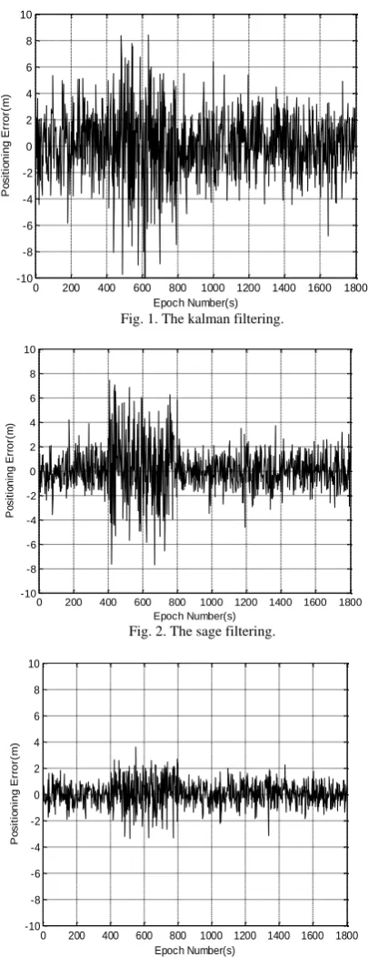
Epoch Number(s) Fig. 1. The kalman filtering.
0 200 400 600 800 1000 1200 1400 1600 1800 -10
-8 -6 -4 -2 0 2 4 6 8 10
P
o
si
ti
o
n
in
g
E
rr
o
r(
m
)
Epoch Number(s)
Fig. 2. The sage filtering.
0 200 400 600 800 1000 1200 1400 1600 1800 -10
-8 -6 -4 -2 0 2 4 6 8 10
P
o
si
ti
o
n
in
g
E
rr
o
r(
m
)
Epoch Number(s)
Fig. 3. The Sage filtering considering the model systematic errors.
It can be seen from Fig. 1 to Fig. 3, between 400~800s. For the comparison purpose, experiments were conducted to estimate the dynamic positioning error of the aircraft at the same conditions by the proposed filtering method as well as the existing methods such as the kalman filtering and the Sage filtering, respectively.
Fig. 1 shows the filtering result obtained by the kalman filtering. It can be seen that there are obvious oscillations in the filtering curve, and the positioning error is within [ 10m 8.2m] , . This shows the kalman filtering is significantly influenced by the disturbances of the kinematic model error.
Fig. 2 shows the filtering result generated by the Sage filtering. The positioning error can be control with
[ 7.8m 7.8m] , , which is much smaller than that by the kalman filtering. This demonstrates that the Sage filtering has the capability to restrain the disturbances of the kinematic model error and the filtering performance is much better in comparison with the Kalman filtering.
Fig. 3 shows the filtering result obtained by the Sage filtering considering the model systematic errors method. It can be seen that there is no obvious oscillation in the filtering curve, and the curve is almost in the stable state during the flight time. The positioning error is control with [ 3.5m 3.8m] , , which is much smaller than that obtained by the Sage filtering.
This demonstrates the proposed method can effectively resist the disturbances caused by the kinematic model errors. Comparing Fig. 3 with Fig. 1 and Fig. 2, it can be seen that the proposed method not only has inhibiting ability, but also has much higher positioning accuracy than the kalman and Sage filtering. However, kinematic model systematic error is not a constant, sometimes if only use the constant systematic error, it cannot completely eliminate the influence of the non-constant systematic errors for filtering result.
VI. CONCLUSION
This new algorithm of Sage filtering considering the model systematic errors adopts Sage filtering established to estimate the kinematic model systematic error as well as the covariance matrices of observation residual vector, predicted residual vector, and predicted state vector within a moving time window. In addition, the model systematic errors can be compensated by correcting predicted residuals and observation residuals. Experiment results and comparison analysis with the existing methods demonstrate that the proposed method of Sage filtering considering the model systematic errors can effectively resist the disturbances of the kinematic model error. The future research work will focus on how to completely eliminate the influence of the non-constant systematic errors for filtering result.
REFERENCES
[1] Y. Yang and T. Xu, “An adaptive kalman filter based on sage windowing weights and variance components,” The Journal of Navigation, vol. 56, no. 2, pp. 231-240, 2003.
[2] T. Xu, N. Jiang, and Z. Sun, “An improved adaptive sage filter with applications in GEO orbit determination and GPS kinematic positioning,” Science China Physics, Mechanics & Astronomy, vol. 55, no. 5, pp. 892-898, 2012.
[3] Y. Yang, Adaptive Navigation and Kinematic Positioning, 1st ed. Surveying and mapping press, China, 2006.
[4] H Tian and X. Zhu, “A simaplied SAGE-HUSA Kalman filtering algorithm,” Journal of Projectiles, Rockets, Missiles and Guidance, vol. 31, no. 1, pp. 75-77, 84, 2011.
[5] Y. Yang and S Zhang, “Adaptive fitting of systematic errors in navigation,” Journal of Geodesy, vol. 79, no. 1-3, pp. 43-49, 2005. [6] X. Cui and Y. Yang, “Adaptively robust filter with classified adaptive
factors,” Progress in Natural Science, vol. 16, no. 8, pp. 846-851, 2006. [7] W. Gao, Y. Yang, X. Cui and S. Zhang, “Application of adaptive kalman filtering algorithm in IMU/GPS integrated navigation system,” Geo-Spatial Information Science, vol. 10, no. 1, pp. 22-26, 2007. [8] Y. Yang and X. Cui, “Adaptively robust filter with multi adaptive
factors,” Survey Review, vol. 40, no. 309, pp. 260-270, 2008. [9] S. Gao, Y. Gao, Y. Zhong, and W. Wei, “Random weighting estimation
[10] S. Gao and W. Wei, “A new and efficient method for random weighting estimation of kinematic model systematic error,” Journal of Northwestern Polytechnical University, vol. 29, no. 6, pp. 839-843, 2011.
[11] Z. Feng, G. Gao, L. Chen, and Y. Jiao, “Random weighting fitting method of systemic errors and covariance matrices in dynamic model,” Systems Engineering and Electronics, vol. 34, no.2, pp. 348-352, 2012. [12] K. R. Koch, Parameter Estimation and Hypothesis Testing in Linear
Models, Second Edition, Berlin: Springer, 1999.
Yi Gao was born in Shaanxi province, China, in 1978. She received the B.S. degree from the School of Automaticion of Northwestern Polytechnical University China, Xi'an, in 2002 and the M.S. degree from the School of Automaticion of Northwestern Polytechnical University China, Xi'an, in 2008. She got the doctor's degree from the School of Automaticion of Northwestern Polytechnical
University China, Xi'an, in 2012. She is a teacher in school of electronic engineering Xian Shi You University from October 8, 2014. Her research interests include automation, navigation, information engineer and control.