CSUSB ScholarWorks
CSUSB ScholarWorks
Electronic Theses, Projects, and Dissertations Office of Graduate Studies
12-2016
Regular Round Matroids
Regular Round Matroids
Svetlana Borissova
California State University - San Bernardino
Follow this and additional works at: https://scholarworks.lib.csusb.edu/etd
Part of the Other Mathematics Commons
Recommended Citation Recommended Citation
Borissova, Svetlana, "Regular Round Matroids" (2016). Electronic Theses, Projects, and Dissertations. 423.
https://scholarworks.lib.csusb.edu/etd/423
A Thesis
Presented to the
Faculty of
California State University,
San Bernardino
In Partial Fulfillment
of the Requirements for the Degree
Master of Arts
in
Mathematics
by
Svetlana Borissova
A Thesis
Presented to the
Faculty of
California State University,
San Bernardino
by
Svetlana Borissova
December 2016
Approved by:
Dr. Jeremy Aikin, Committee Chair Date
Dr. Rolland Trapp, Committee Member
Dr. Belisario Ventura, Committee Member
Dr. Charles Stanton, Chair, Dr. Corey Dunn
Department of Mathematics Graduate Coordinator,
Abstract
A matroid M is a finite setE, called the ground set ofM, together with a notion of what
it means for subsets of E to be independent. Some matroids, called regular matroids,
have the property that all elements in their ground set can be represented by vectors over
any field. A matroid is called round if its dual has no two disjoint minimal dependent
sets. Roundness is an important property that was very useful in the recent proof of
Rota’s conjecture, which remained an unsolved problem for 40 years in matroid theory.
Acknowledgements
I would like to express my sincere gratitude to my thesis advisor, Dr. Jeremy
Aikin, for showing me continuous support, generously sharing his knowledge and
pro-fessional experience, teaching me to set my goals high and being an example of a true
mathematician.
I also want to thank my thesis committee members, Dr. Rolland Trapp and Dr.
Belisario Ventura, for their expertise and encouragement.
There are many more people in CSUSB math department who also helped me
on my journey. I would like to express my gratitude to the department chair, Dr. Charles
Stanton; MA program coordinator, Dr. Corey Dunn, whose classes were the most positive
and interesting; my great professors, Dr. Zahid Hasan, Dr. Yuichiro Kakihara, Dr.
Giovanna Llosent, Dr. Min-Lin Lo, Dr. Shawn McMurran, Dr. Chetan Prakash and Dr.
J. Paul Vicknair, who never ceased to amaze me with their knowledge and passion for
math; department administrators, Leeanne Richardson, Allison Torres and Ana Sanchez,
for always being friendly and supportive.
Finally, I would like to thank my family for believing in me and showing me
support since the time when earning master’s degree in mathematics was just a wild
Contents
Abstract iii
Acknowledgements iv
List of Figures vi
1 Introduction 1
2 Classes of Matroids 10
2.1 Graphic Matroids . . . 10
2.2 Cographic Matroids . . . 17
2.3 Representable Matroids . . . 18
2.3.1 Basic Definitions and Examples . . . 18
2.3.2 Binary Matroids . . . 21
2.3.3 Regular Matroids . . . 23
3 Matroid Constructions 25 3.1 Duality . . . 25
3.2 Minors . . . 27
3.3 Series and Parallel Connection . . . 27
4 Regular Round Matroids 34 4.1 Round Matroids . . . 34
4.2 Seymour’s Decomposition Theorem . . . 38
4.3 The Operation of Direct Sum . . . 38
4.4 The Operation of 2-sum . . . 40
4.5 The Operation of 3-sum . . . 43
5 Conclusion 47
List of Figures
1.1 Different representations of the same matroid-dependence structure. . . . 2
1.2 MatroidM(E,I) with loopd. . . 5
1.3 Simplification of matroid M. . . 6
1.4 GraphGfor matroid N(G). . . 7
1.5 Relationships between certain classes of matroids. . . 7
2.1 A graphG. . . 11
2.2 A simple graphsi(G). . . 11
2.3 Spanning subgraph of graphG from Ex. 2.2. . . 12
2.4 A connected graph and disconnected graph. . . 13
2.5 The blocks of graphH. . . 13
2.6 Subdivision of graphG. . . 14
2.7 The complete graphK5. . . 14
2.8 The complete bipartite graphK3,3. . . 15
2.9 Planar graphs. . . 15
2.10 A graph and its cycle matroid. . . 16
2.11 MatrixA. . . 19
2.12 Standard representative matrix for M. . . 20
2.13 Reduced standard representative matrix for M. . . 21
2.14 The circuit incidence matrix of matroid M from Ex.1.11. . . 21
2.15 Matrix (a) and graph (b) representations of matroid M. . . 22
2.16 Row spaceR(A) of matrix A. . . 22
2.17 Matrix representation for regular matroid R10. . . 23
3.1 GraphG. . . 26
3.2 Parallel extensions and series extensions. . . 28
3.3 A series extension that is not a subdivision. . . 28
3.4 Series and parallel connection in graphs. . . 29
3.5 Series and parallel connections of two matroidsU2,4. . . 30
3.6 Matrix representation ofP(M1, M2). . . 31
3.7 Matrix representation ofS(M1, M2). . . 32
4.2 The parallel and series connections and 2-sum of graphs. . . 41
4.3 Matrix representation ofP(M1, M2). . . 42
4.4 Representation forM1⊕2M2 =P(M, N)\p. . . 42
4.5 The 3-sum ofG1 andG2. . . 43
4.6 Matrix representations of matroidsM1 and M2. . . 46
4.7 Matrix representation of the 3-sum of matroidsM1 andM2. . . 46
5.1 Matrix representation of projective geometryP G(2,2). . . 48
5.2 Fano Plane. . . 48
Chapter 1
Introduction
Matroids were first introduced by the American mathematician Hassler Whitney
in his paper “On the abstract properties of linear dependence” published in American
Journal of Mathematics in 1935 [Whi35]. In that paper Whitney defined a “system”
obeying the following two properties of linear dependence in a matrix:
(a) Any subset of an independent set is independent.
(b) IfNp andNp+1 are independent sets ofpandp+ 1 columns respectively, then
Np with some column ofNp+1 forms an independent set of p+ 1 columns.
These two properties not always describe a matrix, so Whitney named any
system obeying these properties a “matroid”. Moreover, Whitney emphasized a close
connection between matroids and graphs. As matroids were studied further, it has been
recognized that matroids also combine ideas from combinatorics, finite geometry and
abstract algebra. The fact that matroids provide many connections between the various
branches of mathematics has been attracting a lot of mathematicians and has made
matroid theory one of the most active research areas in mathematics today.
The modern definition of a matroid is given in terms of three independent set
axioms:
Definition 1.1 (Matroid). A matroid M is defined by a finite setE, called the ground set, and a collectionI of subsets of E that satisfy the following axioms:
(I2) If I ∈ I and I0 ⊆I, thenI0 ∈ I; (Closed under subsets)
(I3) If I1 and I2 are inI and |I1|<|I2|, then there is an element eofI2−I1 such that I1∪e∈ I. (Augmentation)
Any subset of E that belongs to I is called an independent set. Subsets of E
that are not independent are called dependent.
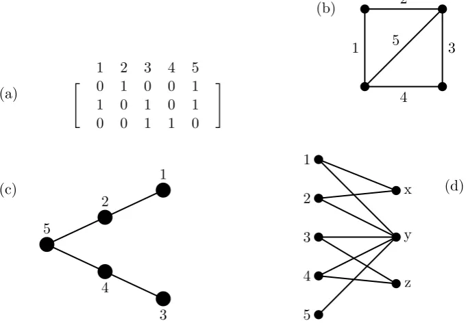
Figure 1.1 illustrates how the same matroid-dependence structure can be
repre-sented by the objects from different areas of mathematics.
(a)
1 2 3 4 5
" 0 1 0 0 1 #
1 0 1 0 1
0 0 1 1 0
5 2
1 3
4 (b)
1
2
5
4
3 (c)
1
2
3
4
5
x
y
z
(d)
Figure 1.1: Different representations of the same matroid-dependence structure.
All these objects represent the same matoroid M(E,I) with ground set E =
{1,2,3,4,5} and collection I of independent subsets of E consisting of the empty set,
all single elements, all pairs of elements and all triples of elements, except {1,2,5} and
{3,4,5}. Clearly, the notion of independence between the elements in each object is
different. In matrix (a), independent set corresponds to any subset of columns that
are linearly independent. A matroid whose ground set is a set of vectors is called a
representable matroid. In graph (b), independent set corresponds to an acyclic subset of
cycle matroid. We will study representable and cycle matroids more closely in Chapter
2.
Picture (c) is a geometric representation of matroid M(E,I). It is based on
a point-line incidence geometry, so each element of the ground set is represented by a
point and every subset of points of size 1 or 2 and any set of points that does not contain
a 3-point line is considered independent. In a matroid, an independent set consisting
of four elements is represented geometrically by four non-coplanar points. Geometric
representation of matroids is discussed in great detail by Gary Gordon and Jennifer
McNulty in their book “Matroids: A Geometric Introduction” [GM11].
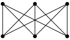
Picture (d) reflects a bipartite graph. A close connection between matroids and
matchings in bipartite graphs was discovered by the German-born British mathematician
Richard Rado in the 1940s. A bipartite graph is a graph where the set of vertices can
be partitioned into two sets so that no edges of the graph join two vertices in the same
part of the partition. A subset of edges is called a matching if no two edges in the
set share a vertex. The collection of all the possible matchings gives us the connection
to matroids. In fact, an independent set I of a matroid corresponds to the subset X
of the vertices in the same part of the partition that can be matched in a bipartite
graph, i.e. there is a matching in which every edge has one endpoint in X. A matroid
associated with matchings in a bipartite graph is called a transversal matroid. Finding
matchings in bipartite graphs is a very important and well-studied topic in combinatorics
with applications in scheduling problems, which illustrates the diversity and versatility
of matroids.
We will now define other important attributes of matroids. All the matroid
notation throughout this thesis will follow Oxley [Oxl11].
Definition 1.2 (Rank). LetM = (E,I) be a matroid and letA be a subset ofE. Then the rank of A, writtenr(A), is the size of the largest independent subset of A:
r(A) := max
I⊆A{|I|:I ∈ I}.
The rank function r satisfies the inequalityr(X∪Y) +r(X∩Y)≤r(X) +r(Y), making
r a submodular function.
B={B ∈ I |B⊆A∈ I implies B=A}.
Definition 1.4 (Circuit). Let M be a matroid. If C is dependent, but every proper subset of C is independent, we call C a circuit in the matroid. Thus, C is a minimal
dependent set:
C ={C⊆E|C /∈ I and if I (C thenI ∈ I}.
Definition 1.5 (Flat). Let E be the ground set of a matroid M. A subset F ⊆ E is a flat if r(F ∪ {x}) > r(F) for any x /∈ F. In other words, a flat is a subset of E that
is rank-maximal. Thus, adding a new element to a flat increases its rank. A flat is also
called aclosed set ofM.
Definition 1.6(Hyperplane). LetE be the ground set of a matroidM. A subsetH ⊆E
is ahyperplane ifH is a flat of M and if r(H) =r(M)−1.
Definition 1.7 (Closure operator). LetM be an arbitrary matroid having ground setE
and rank r. Then theclosure operator of M is the function cl from 2E into 2E defined,
for all X ⊆E, by
cl(X) ={x∈E :r(X∪x) =r(X)}.
We call cl(X) theclosure of X.
Definition 1.8 (Spanning Set). A subset X of E(M) is aspanning set ofM ifcl(X) =
E(M). Equivalently, a subset X is a spanning set if it contains a basis.
Among other special features of a matroid are loops and coloops. A coloop (or
isthmus) is an element that is in every basis of the matroid. A loop is an element that is
in no basis. That is, a loop is a dependent singleton or a circuit of size 1.
Example 1.9. Figure 1.2 shows different representations of a loopdin matroidM(E,I) with ground setE ={a, b, c, d}and collection of independent setsI ={{a},{b},{c},{a, b},
(a) Matrix representation
a b c d
1 0 1 0
0 1 1 0
c b
a
d
(b) Graph representation
a b c
d
(c) Geometric representation
Figure 1.2: Matroid M(E,I) with loopd.
Moreover, if f and g are non-loop elements of a matroid M such that {f, g} is
a circuit, then f and g are parallel in M. A parallel class of M is a maximal subset X
of E(M) such that any two distinct members ofX are parallel and no member of X is a
loop. A parallel class is trivial if it contains just one element. If we delete all the loops
from M and then, in each non-trivial parallel class X, we distinguish one element and
delete all the other elements of X, the matroid we obtain is uniquely determined up to
renaming of the distinguished elements. We denote this matroid bysi(M) and call it the
simplification of M. IfM has no loops and no non-trivial parallel classes, it is called a
simple matroid.
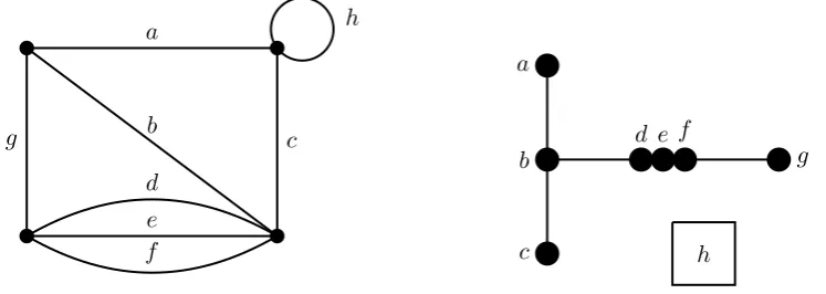
Example 1.10. Consider matroid M as shown on Figure 1.3(a). This matroid has a non-trivial parallel class X = {d, e, f} and a loop h. If we delete loop h and two out
of three elements in parallel class X, then we obtain the simplification of M, matroid
b a
c
d e f
g
(a) Matroid M h
b a
c
d
g
(b) Matroidsi(M)
Figure 1.3: Simplification of matroid M.
Next we are going to define an isomorphism between two matroids.
Example 1.11. Let G be the graph shown in Figure 1.4 and let matroid N = N(G).
ThenE(N) ={e1, e2, e3, e4, e5, e6, e7, e8,}andC(N) ={{e8}{e4, e5},{e4, e6},{e5, e6},{e1, e2, e3},
{e2, e4, e7},{e2, e5, e7},{e2, e6, e7}}. Comparing matroid N with matroidM from
Exam-ple 1.10, we see that there is a bijectionφfrom{a, b, c, d, e, f, g, h}to{e1, e2, e3, e4, e5, e6, e7, e8,}
defined by:
φ(a) =e1
φ(b) =e2
φ(c) =e3
φ(d) =e4
φ(e) =e5
φ(f) =e6
φ(g) =e7
φ(h) =e8,
such that a set C is a circuit inM if and only if φ(C) is a circuit inN. Equivalently, a
setI is independent inM if and only ifφ(I) is independent inN. Thus, the matroidsM
e1
e7
e2
e6 e4
e5
e3 e8
Figure 1.4: Graph Gfor matroid N(G).
Formally, two matroidsM1 and M2 areisomorphic, written M1 ∼=M2, if there
is a bijection φ from E(M1) to E(M2) such that, for all X ⊂ E(M1), the set φ(X) is
independent in M2 if and only ifX is independent inM1. We call such a bijection φan
isomorphism fromM1 toM2.
A matroid that is isomorphic to the cycle matroid of a graph is calledgraphic.
Therefore, matroid M in Example 1.11 is graphic.
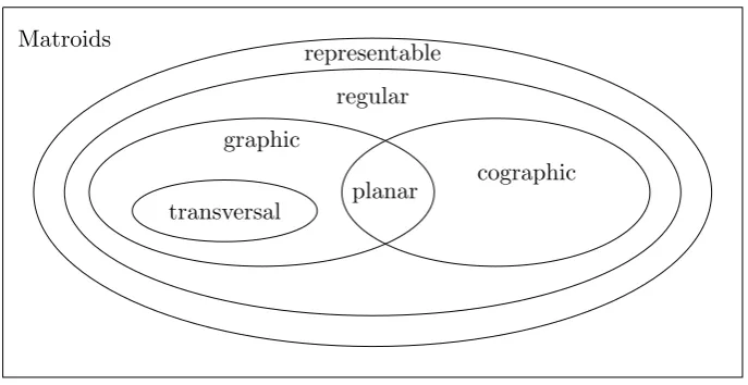
Besides representable, graphic and transversal matroids there is another class
of matroids that will be of primary interest in this thesis: regular matroids. Regular
matroids are a subclass of representable matroids. Their unique feature is that they can
be represented by a matrix over any field. Figure 1.5 helps to better understand the
relationships between all these classes.
Matroids
representable
regular
graphic
cographic
transversal planar
Two other classes of matroids in Figure 1.5 that we have not yet mentioned
are cographic and planar. To define cographic matroids, we first introduce the notion
of duality. Given matroid M on the ground set E, we say that the dual matroid M∗ is the matroid on the same ground set E, such that B(M∗) = {E−B :B ∈ B(M)}. The duals of graphic matroids are called cographic matroids. If a matroid is both graphic and
cographic, then it is isomorphic to the cycle matroid of a planar graph, a graph that can
be drawn on a plane without crossing edges. Such matroids are called planar.
In this project we will focus on regular matroids that have the additional
prop-erty of being round. Round matroids are an analogue of complete graphs and have the
following characterizations:
(i) MatroidM is round if and only if it has no two disjoint cocircuits, where cocircuit is defined by a set C∗ ∈E, such thatC∗ is a circiut in the dual matroidM∗.
(ii) Matroid M is round if and only if every cocircuit is spanning, i.e. every cocircuit contains a basis.
(iii) Matroid M is round if and only if it cannot be written as the union of two proper flats.
Since regular matroids include graphic and cographic matroids, it would be
interesting to know what specific characteristics must be possessed by matroids from
these two classes in order to be round. We will answer this question in Section 4.2.
Next we want to see if there are regular round matroids that are neither graphic
nor cographic. To investigate this matter we are going to use one of the very important
results in matroid theory that was presented by a modern British mathematician, Paul
Seymour. In 1980 Paul Seymour published an article titled “Decomposition of
Regu-lar Matroids” in which “it is proved that every reguRegu-lar matroid may be constructed by
piecing together graphic and cographic matroids and copies of a certain 10-element
ma-troid” [Sey80]. This result won Paul Seymour his first P´olya Prize and is now known as
Seymour’s Decomposition Theorem stated below.
is either graphic, cographic or isomorphic to R10, and each of which is isomorphic to a
minor of M.
The operations of direct sum, 2-sum and 3-sum allow one to obtain a new
matroid from two (or more) arbitrary matroids on disjoint ground sets, ground sets with
one element in common and ground sets with a common 3-circuit, respectively. Definitions
of these operations along with our results on obtaining a regular round matroids using
Chapter 2
Classes of Matroids
In this chapter we discuss three important classes of matroids: graphic,
co-graphic and representable matroids.
2.1
Graphic Matroids
There is a close connection between graphs and matroids. To describe this
relationship we first need to define graphs.
Definition 2.1 (Graph). A graph G is a finite nonempty setV of objects called vertices together with a set E of 2-element subsets ofV called edges.
Each edge{u, v}ofV is commonly denoted byuvorvu. Ife=uv, then the edge
eis said to join verticesuandvand verticesuandvare called theadjacent vertices. The
number of vertices that are adjacent to a vertex v is called the degree of v and denoted
by deg v. An edge joining a vertex to itself is called a loop. Two or more edges that join
the same pair of distinct vertices are called parallel edges. A graph G that contains no
loops or parallel edges is called a simple graph. The number of vertices in a graph Gis
the order of Gand the number of edges is the size of G.
Two graphsGandG0areisomorphicif there exists a bijectionσ :V(G)→v(G0) such that two vertices uand v are adjacent inGif and only ifσ(u) andσ(v) are adjaent
inG0.
Graphs are typically represented by diagrams in which each vertex is represented
or curve joining the corresponding small circles.
Example 2.2. Figure 2.1 shows a graph G with vertex setV = {a, b, c, d, e} and edge set E = {ab, ac, ad, bb, bc, bd, cd, cd, cd, de}. Thus the order of this graph G is 5 and its
size is 10. Note that edge bb is a loop and there are three parallel edges joining vertices
c and d.
a
d e
b
c
Figure 2.1: A graph G.
If we delete the loop and all except one of parallel edges in graph G, then we
obtain a simple graph that we denote si(G) (Figure 2.2).
a
d e
b
c
Figure 2.2: A simple graphsi(G).
Other important attributes of graphs are defined below.
Definition 2.3 (Walk). For two (not necessarily distinct) vertices u and v in a graph
G, a u−v walk W in G is a sequence of vertices in G, beginning at u and ending at v
such that consecutive vertices in W are adjacent inG. A walk whose initial and terminal
vertices are distinct is an open walk; otherwise, it is a closed walk. The length of a walk
Definition 2.4 (Path). A walk in a graph G in which no vertex is repeated is called a path.
Definition 2.5 (Cycle). A nontrivial closed walk C = (v=v0, v1, . . . , vk =v), k≥2 in which no edge is repeated and the vertices vi, 1≤i≤k−1, are distinct is called a cycle.
A cycle of length k≥3 is called a k-cycle. A 3-cycle is also referred to as a triangle.
Definition 2.6 (Spanning subgraph). A graph H is said to be a subgraph of a graph G if V(H)⊆V(G) andE(H)⊆E(G). If V(H) =V(G), then H is a spanning subgraph.
Example 2.7. Figure 2.3 below shows a spanning subgraph of a graphGfrom Example 2.2. Observe that this subgraph contains a 3-cycle (or triangle) C = (a, c, d, a).
a
d e
b
c
Figure 2.3: Spanning subgraph of graphG from Ex. 2.2.
We can classify graphs in terms of connectivity. We say that graphGisconnected
if for any two verticesuandv, there is au−vpath inG. A graph that is not connected is
calleddisconnected. A maximal connected subgraphH of a graphGis called acomponent
of G.
There are different degrees of connectedness in graphs. For example, some
graphs are so slightly connected that they can be disconnected by the removal of a single
vertex or a single edge called cut-vertex or abridge, respectively. A nontrivial connected
graph that has no cut-vertices is callednonseparable. A maximal nonseparable subgraph
B of a nontrivial connected graph Gis called ablock of G.
Example 2.8. The graph H in Figure 2.4 is connected since there is a path between every two vertices in H. On the other hand, the graph G is disconnected since, for
x1
x2
x3
x5
x4
x6
H
y1 y2
y4
y5
y7
y3
y8 y6
G
Figure 2.4: A connected graph and disconnected graph.
Three blocks B1, B2, B3 of graphH are shown in Figure 2.5 below.
x1
x2
x3
x5 B1
x3 x4
B2
x5
x6 B3
Figure 2.5: The blocks of graph H.
One of the operations that we can perform on a graph is a subdivision. A graph
H is asubdivision of a graphGif eitherH=GorH can be obtained fromGby inserting
vertices of degree 2 into the edges of G. Thus for the graph Gin Figure 2.6, graph H is
G H
Figure 2.6: Subdivision of graphG.
Among the well-studied classes of graphs are complete and bipartite graphs. A
complete graph is a simple undirected graph in which every pair of distinct vertices is
connected by a unique edge (Figure 2.7). Complete graphs are usually denoted by Kn,
where nrepresents a number of vertices.
Figure 2.7: The complete graphK5.
A nontrivial graph Gis abipartite graph if it is possible to partitionV(G) into
two subsets U and W, called partite sets, such that every edge of Gjoins a vertex of U
and a vertex ofW. A bipartite graph having partite setsU andW is acomplete bipartite
graph if every vertex ofU is adjacent to every vertex ofW. If the partite setsU andW
of a complete bipartite graph contain sandtvertices, then this graph is denoted byKs,t
orKt,s. Figure 2.8 shows the complete bipartite graph K3,3. Observe that this graph has
Figure 2.8: The complete bipartite graph K3,3.
Another class of graphs is planar graphs. A graphGis called a planar graph if
G can be drawn in the plane without any two of its edges crossing. Any plane drawing
of G divides the plane into regions. Examples of planar graphs include graphs obtained
from Platonic solids (Figure 2.9).
Tetrahedron Cube Octahedron
Figure 2.9: Planar graphs.
When considering a plane drawing of graphGof a polyhedron, the faces of the
polyhedron become the regions of G, one of which is the exterior region ofG.
There exist many interesting results for planar graphs, which can sometimes be
used to determine whether a graph is planar or nonplanar. These are some of them:
• For every connected planar graph of ordern, sizem, and havingr regions,n−m+
r = 2 (The Euler Identity).
• If Gis a planar graph of order n≥3 and sizem, then m≤3n−6.
• Every complete graph Kn of ordern≥5 is nonplanar.
• Every planar graph contains a vertex of degree 5 or less.
Proofs of these properties can be found in most graph theory texts.
Another important result for planar graphs was proved by the well-known
Pol-ish topologist Kazimierz Kuratowski in 1930. It provides both necessary and sufficient
conditions for a graph to be planar. Kuratowski’s Theorem is stated below and will be
referred to in the later chapters. A proof of Kuratowski’s Theorem can be found in the
book titled “Chromatic Graph Theory” by Gary Chartrand and Ping Zhang [CZ09].
Theorem 2.9 (Kuratowski’s Theorem). A graph G is planar if and only of G contains no subgraph that is a subdivision of K5 or K3,3.
We are now ready to connect graphs to matroids. For any given graphG there
is a matroid M(G) associated with it, such that the ground set E corresponds to the
set of edges of G and collection of independent sets I corresponds to the collection of
all subsets of edges that are acyclic. Thus, the circuits of such matroid are precisely the
cycles of the graph. The matroidM(G) is called the cycle matroid ofG.
Example 2.10. Consider the graph on the left in Figure 2.10. Its cycle matroid is shown on the right.
a
g b
f d
e
c h
b a
c
d e f
g
h
Figure 2.10: A graph and its cycle matroid.
Even though every graph corresponds to a matroid, not every matroid comes
from some graph. Matroids that do arise as cycle matroids of graphs are called graphic.
The following lemmas provide two properties of graphic matroids.
Lemma 2.11. Let Gand H be graphs. ThenM(G)=∼M(H) if and only if G∼=H. Proof. LetGandHbe graphs andM(G) andM(H) be graphic matroids associated with
that two verticesuandvare adjacent inGif and only ifσ(u) andσ(v) are adjacent inH.
Therefore, there is a bijection ˜σ :E(M(G))→E(M(H)) such that, for allX⊂E(M(G)),
the set ˜σ(X) is independent in M(H) if and only if X is independent in M(G). Thus,
M(G)∼=M(H).
Now, suppose thatM(G) ∼=M(H). Then there is a bijection ˜σ :E(M(G))→
E(M(H)) such that, for allX⊂E(M(G)), the set ˜σ(X) is independent inM(H) if and
only if X is independent in M(G). Therefore, there exists a bijection σ:V(G)→V(H)
such that two verticesuand vare adjacent inGif and only if σ(u) andσ(v) are adjacent
inH. Thus, G∼=H.
Lemma 2.12. Let G be a graph. Then M(si(G)) ∼= si(M(G)), where M is the cycle matroid of G.
Proof. Let G be a graph. Then the graph H = si(G) is obtained by deleting all the
loops and all but one edge in each parallel class in G. Next consider cycle matroid
M(G). Then matroid K = si(M(G)) is obtained by deleting all the loops and all but
one element in each non-trivial parallel class in M. Since M(G) is a cycle matroid, then
loops in matroid M correspond to the loops in graph G. Moreover, each non-trivial
parallel class in matroidM corresponds to a set of parallel edges in graphG. Therefore,
K ∼=M(H) and M(si(G))∼=si(M(G)).
2.2
Cographic Matroids
The definition of cographic matroids is based on the notion of duality. Given
matroid M on the ground setE, we say that thedual matroid M∗ is the matroid on the same ground set E, such that B(M∗) ={E−B :B ∈ B(M)}. We will study duality in more detail in Chapter 3.
Definition 2.13(Cographic Matroid). The dual of a graphic matroid is called a cographic matroid.
One of the properties of cographic matroids inherited from graph theory is that
a graphic matroid is cographic if and only if the corresponding graph is planar.
One more property of cographic matroids is outlined in Lemma 2.14 below.
Proof. Let matroidsi(M) be the simplification of matroid M. Therefore, si(M) is
ob-tained by deleting all the loops and all but one element in each parallel class in matroid
M. Suppose that si(M) is cographic. Then there exists a dual matroid (si(M))∗ that is a cycle matroid of some graph G. To restore matroid M from matroid si(M) we would
need to add all the deleted loops and elements from parallel classes to matroid si(M).
This corresponds to subdividing edges and adding leaves in graph G. Since this new
graph corresponds to the dual matroid M∗, then matroidM is cographic.
2.3
Representable Matroids
2.3.1 Basic Definitions and Examples
The fundamental class of representable matroids is directly connected with
ma-trices and their properties. In fact, any finite set of vectors produces a matroid.
Lemma 2.15. Let E be the set of column labels of anm×nmatrix A over a fieldF, and let I be the set of subsets of X of E for which the multiset of columns labeled by X is a
set and is linearly independent in the vector space V(m,F). Then (E,I) is a matroid.
The matroid obtained from the matrixA is called the vector matroid of A and
denoted by M[A]. Moreover, any matroid M that is isomorphic to the vector matroid
of a matrix D over a field F is representable over F or F-representable, and D is a
representation forMoverFor anF-representation forM. A matroid that is representable
over some field is called representable.
We already stated that ground setE of representable matroidM[A] corresponds
to the set of columns of matrix A and collection of independent sets I corresponds to
the linearly independent sets of columns of matrix A. Below is a list of other important
attributes of representable matroid and their correlation with the matrix:
• Bases (B) correspond to the maximal linearly independent sets of columns.
• Circuits (C) correspond to the minimal linearly dependent sets of columns.
• Rank (r) corresponds to the rank of the matrix.
• Hyperplanes (H) correspond to flats of rank one less than the rank of the matrix.
• Closure correspond to the linear span.
• Spanning sets (S) correspond to the subsets of columns whose linear span contains
all the columns of the matrix.
Next example illustrates these relations.
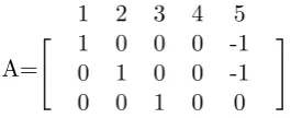
Example 2.16. Consider matrix A in Figure 2.9 represented over the field R of real numbers.
A=
1 2 3 4 5
" 1 0 0 0 -1 #
0 1 0 0 -1
0 0 1 0 0
Figure 2.11: MatrixA.
Then the vector matroidM[A] on ground setE={1,2,3,4,5}has the following
attributes:
– Rank r(M[A]) = 3 is the rank of matrix A.
– Collection of independent sets I ={∅,{1},{2},{3},{5},{1,2},{1,3},{1,5},
{2,3},{2,5},{3,5},{1,2,3}} represent the collection of subsets of linearly
in-dependent columns of matrix A.
– BasesB={{1,2,3},{1,3,5},{2,3,5}} is the maximal set of columns that are linearly independent.
– Collection of circuits C ={{1,2,3},{4}} corresponds to the minimal linearly dependent sets of columns of matrix A. In general, these are harder to
recog-nizance in a matrix.
– Subcollection of hyperplanes of M[A] that can be found using the above rep-resentation of matrix A is {{2,3,4},{1,3,4},{1,2,4,5},}. Recall that
hyper-plane is viewed as a set of columns of rank 1 less than the rank of a matrix
and that is equal to its linear span. If we fix any non-zero row in matrix A,
then the set of columns with zero entries in that row forms a subspace of the
In general,M[A] does not uniquely determine A. A vector matroidM remains
unchanged if one performs any of the following elementary row operations onA:
(i) Interchange two rows.
(ii) Multiply a row by a non-zero member of F.
(iii) Replace a row by the sum of that row and another.
(iv) Adjoin or remove a zero row.
(v) Interchange two columns (the labels moving with the columns).
(vi) Multiply a column by a non-zero member of F.
(vii) Replace each matrix entry by its image under some automorphism ofF.
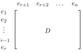
Assume that the matrix A is non-zero. Using the above elementary row
oper-ations, we can reduce A to the form [Ir|D] where Ir is the r×r identity matrix and D
is some r×(n−r) matrix over F. Clearly, r =r(M). If we label the columns of [Ir|D]
by e1, e2, ..., en, then{e1, e2, ..., er}is a basisB ofM. Moreover, it is natural to label the
rows of D, in order, by e1, e2, ..., er. Thus M[A] can be represented both by the matrix
[Ir|D], whose columns are labelede1, e2, ..., en(Figure 2.10), and by the matrixD, whose
row are labelede1, e2, ..., erand whose columns are labeleder+1, er+2, ..., en(Figure 2.11).
Matrix [Ir|D] is called astandard representation matrix for M and matrixD is called a
reduced standard representative matrix.
e1 e2 . . . er er+1 er+2 . . . en
Ir D
er+1 er+2 . . . en e1 e2 .. . D
er−1 er
Figure 2.13: Reduced standard representative matrix for M.
Besides the standard representative matrix, a vector matroid M can be
repre-sented by the circuit incidence matrix. If M is a matroid on the set {1,2, . . . , n} such
thatC(M) ={C1, C2, . . . , Cm}, then the circuit incidence matrixA(C) ofM is them×n
matrix [aij] in which aij is 1 or 0 depending on whether j is or is not inCi.
Example 2.17. Consider matroid M from Example 1.10. It has ground set E(M) = {a, b, c, d, e, f, g, h}and the set of circuitsC(M) ={C1, C2, . . . , C8}, whereC1 ={h}, C2=
{d, e}, C3 = {d, f}, C4 = {e, f}, C5 = {a, b, c}, C6 = {b, d, g}, C7 = {b, e, g}and C8 =
{b, f, g}. The circuit incidence matrixA(C) of M is the 8×8 matrix shown below.
a b c d e f g h
C1 0 0 0 0 0 0 0 1
C2 0 0 0 1 1 0 0 0
C3 0 0 0 1 0 1 0 0
C4 0 0 0 0 1 1 0 0
C5 1 1 1 0 0 0 0 0
C6 0 1 0 1 0 0 1 0
C7 0 1 0 0 1 0 1 0
C8 0 1 0 0 0 1 1 0
Figure 2.14: The circuit incidence matrix of matroidM from Ex.1.11.
The most commonly studied classes of representable matroids are binary, ternary
and regular matroids. Binary and ternary matroids are representable over GF(2) and
GF(3) respectively. A regular matroid is one that can be represented over any field.
2.3.2 Binary Matroids
Binary matroids are representable over GF(2) and have a number of special
have been widely-studied and characterized.
One of the unique properties of binary matroids connects the cocircuit space of
a binary matroid to the row space of a matrix by which it’s represented. In general, the
row space R(A) of an m×n matrix A over a field F is the subspace of V(n,F) that is
spanned by the rows of A. This property is outlined in Lemma 2.16.
Lemma 2.18. Let A be a binary representation of a rank-r binary matroid M. Then the cocircuit space of M equals the row space of A. Moreover, this space has dimension r and
is the orthogonal subspace of the circuit space of M.
Example 2.19. Consider matroidM represented by the binary matrix A and graphG
in Figure 2.13 (a) and (b) respectively.
(a)
A=
1 2 3 4 5
" 0 1 0 0 1 #
1 0 1 0 1
0 0 1 1 0
5 2
1 3
4 (b)
Figure 2.15: Matrix (a) and graph (b) representations of matroid M.
The members of the row spaceR(A) of matrixA are the rows of the following
matrix.
1 2 3 4 5
Row 1 0 1 0 0 1
Row 2 1 0 1 0 1
Row 3 0 0 1 1 0
Row 1 + Row 2 1 1 1 0 0
Row 1 + Row 3 0 1 1 1 1
Row 2 + Row 3 1 0 0 1 1
Row 1 + Row 2 + Row 3 1 1 0 1 0
Row 1 + Row 1 0 0 0 0 0
Figure 2.16: Row spaceR(A) of matrix A.
{{2,5},{1,3,5},{3,4},{1,2,3},{2,3,4,5},{1,4,5},{1,2,4},{∅},}in matroidM. By
find-ing these sets on graph Gwe can check that they represent all possible disjoint unions of
cocircuits.
2.3.3 Regular Matroids
The following statements are equivalent for a matroid M:
(i) M is regular.
(ii) M is representable over every field.
(iii) M is binary and, for some fieldFof characteristic other than two,M isF-representable. Sometimes regular matroids are referred to as unimodular matroids, because
they can be represented by a totally unimodular matrix. A totally unimodular matrix is
a matrix over Rfor which every square submatrix has determinant in the set{−1,0,1}.
Such matrices play an important role in computer science in solving liner programming
problems.
It’s also important to note that every graphic matroid and every cographic
matroid is regular.
One of the well-studied representatives of the class of regular matroids is matroid
R10 that is the vector matroid of the matrixA10 overGF(2) shown on Figure 2.17.
A10=
1 2 3 4 5 6 7 8 9 10
1 1 0 0 1
1 1 1 0 0
I5 0 1 1 1 0
0 0 1 1 1
1 0 0 1 1
Figure 2.17: Matrix representation for regular matroidR10.
The matroidR10 has many attractive features. These are some of them:
• Among regular matoids that are neither graphic nor cographic, the only one with
ten elements and the only simple one of rank at most five.
• Every single-element deletion is isomorphic to M(K3,3), and every single-element
contraction is isomorphic to M∗(K3,3).
Chapter 3
Matroid Constructions
In this chapter we will introduce several different ways of obtaining a new
ma-troid from one or more arbitrary mama-troids.
3.1
Duality
One of the most important properties of matroids is duality.
Definition 3.1 (Dual Matroid). Let M be a matroid on the ground set E. Then the dual matroid M∗ is a matroid on the same ground set E, so that
B(M∗) ={E−B :B ∈ B(M)}.
MatroidM is calledself-dual ifM ∼=M∗ and identically self-dual ifM =M∗. The bases, independent sets, spanning sets, circuits and hyperplanes of the dual matroid
M∗ are related to those ofM as follows:
M∗ M
B is a basis ⇔ E−B is a basis
I is independent ⇔ E−I is spanning
S is spanning ⇔ E−S is independent
C is a circuit ⇔ E−C is a hyperplane
H is a hyperplane ⇔ E−H is a circuit
Another important attribute of a matroid that we can define using duality is a
cocircuit. A cocircuit of a matroidM(E,I) is a setC∗ ⊆E, such thatC∗is a circuit in the dual matroid M∗. Equivalently, we can look at cocircuits as hyperplane complements. In a cycle matroid M(G), each cocircuit corresponds to a minimal edge cut-set of G,
which is a collection of edges whose removal from the graph breaks a component into two
or more pieces. For example, if we take all the edges in a connected graph G that are
incident to a given vertex (that is not a cut-vertex), then we get a cocircuit in M(G).
That cocircuit is the complement of a hyperplane inM(G), because adding another edge
to that hyperplane gives a spanning set.
Example 3.2. Consider graph G shown in Figure 3.1. The vertex cut-set {d, g, j, h} disconnects vertex v4 from the graph. Therefore, {d, g, j, h} is a cocircuit in the cycle
matroidM(G). Observe, that the cocircuit{d, g, j, h}is the compliment of the hyperplane
H ={a, b, c, e, f, i, k, l}, because adding one of the edges d, g, k orh to H will give us a
spanning set.
d
c e
a
f b
h
l
i g
v4
v5 v1
v3 v2
v6
v7 k
j
Figure 3.1: GraphG.
For any representable matroid M[A], cocircuits, viewed as hyperplane
compli-ments, correspond to the subset of columns with non-zero entries in any fixed row of
matrix A. Note that any given representation of a matrix does not provide the entire
collection of cocircuits in a matroid, since performing row operations on the matrix A
will allow us to see more cocircuits, when viewed from this perspective.
One of the properties of duality is outlined in the next result.
Lemma 3.3. If a matroid M is representable over a fieldF, thenM∗ is also representable over F.
In particular, the dual of a binary matroid is binary, and the dual of a ternary
3.2
Minors
Deletion and contraction are two important operations that we can perform on
a matroid. Both operations reduce the size of the matroid by removing an element from
E(M).
Definition 3.4 (Deletion). Let M be a matroid on the ground set E with independent sets I. For e ∈ E (e is not a coloop), the matroid M\e has ground set E − {e} and
independent sets that are those members of I that do not containe. In other words, I is
independent in M\e if and only if e /∈I andI is independent inM.
Definition 3.5(Contraction). LetM be a matroid on the ground setE with independent sets I. For e ∈ E (e is not a loop), the matroid M/e has ground set E − {e} and
independent sets that are formed by choosing all those members of I that contain e, and
then removing efrom each set. In other words,I− {e}is independent in M/eif and only
if e∈I and I is independent in M.
Combining and iterating these operations produces aminor of the original
ma-troid.
3.3
Series and Parallel Connection
The operations of joining electrical components in series and in parallel are
fundamental in electrical network theory. There also exist the corresponding operations
for graphs that naturally extend to matroids. First, we are going to investigate these
operations for graphs.
Example 3.6. Consider graphs G,G1 and G2 as shown in Figure 3.2. Graphs G1 and
G2 were obtained from graphGby adding the edgef in parallel with edgeeandin series
e
G
e f
G1
e
f
G2
Figure 3.2: Parallel extensions and series extensions.
For an arbitrary graphG, these operations are defined as follows: G0 is aparallel extension of G, or, equivalently, Gis a parallel deletion of G0 ifG0 has a two-edge cycle {e, f} such thatG0\f =G. If, instead, {e, f} is a two-edge cocycle ofG0, andG0/f =G, then G0 is a series extension of G, and G is a series contraction of G0. Note, that not every series extension consists of replacing an edge by a path of length two.
e e
f
Figure 3.3: A series extension that is not a subdivision.
The operations of series and parallel extensions in graphs can be generalized to
matroids. In particular, if M\f = N and f is in a 2-circuit of M, thenM is a parallel
extension of N, and N is a parallel deletion of M. If, instead, M/f = N and f is in a
2-cocircuit ofM, thenM is aseries extension of N, and N is a series contraction ofM.
Clearly M is a parallel extension of N if and only if M∗ is a series extension of N∗. A series class of M is a parallel class ofM∗; it is non-trivial if it has at least two elements. Moreover, a series minor of a matroidM is a matroidN that is obtained from M by a
series of deletions and series contractions. If, instead, N can be obtained from M by a
sequence of contractions and parallel deletions, thenN is a parallel minor ofM. Clearly,
M1 is a parallel minor ofM2 if and only ifM1∗ is a series minor of M2∗.
The operations of series and parallel extension for graphs are special cases of the
operations of series and parallel connection of graphs. We will define these operations
and show how they naturally extend to matroids. For each iin {1,2}, let pi be an edge
vi. To form the series and parallel connections of G1 and G2 with respect to the direct
edges p1 and p2, we begin by deleting p1 from G1 and p2 from G2; we then identify u1
and u2 as the vertexu. To complete the series connection, we add a new edge p joining
v1 and v2. The parallel connection is completed by identifying v1 and v2 as the vertexv
and then adding a new edge p joining u and v. Thus, unless exactly one of p1 and p2 is
a loop, the parallel connection is obtained by simply identifying p1 and p2 so that their
directions agree.
Example 3.7. The graphsGandHin Figure 3.4 are, respectively, the series and parallel connections of the graphsG1 and G2 with respect to the directed edgesp1 and p2.
p1 u1
v1 G1
p2 u2
v2
G2
p u
v1
v2 G
p u
v H
Figure 3.4: Series and parallel connection in graphs.
Now we will show how series and parallel connection in graphs can be extended
to matoroids. Let CS and CP denote the collection of circuits of the cycle matroids of
the series and parallel connections of the graphs G1 and G2. Then in the last example,
and indeed in general, it is not difficult to specify CS and CP in terms of C(M(G1)) and
C(M(G2)). Writing M1 forM(G1) andM2 forM(G2) and assuming neitherp1 norp2 is
a loop or a cut edge, we have
CS =C(M1\p1)∪ C(M2\p2)∪ {(C1−p1)∪(C2−p2)∪p:pi ∈Ci ∈ C(Mi) for each i}
CP =C(M1\p1)∪ {C1−p1∪p:p1 ∈C1 ∈ C(M1)} ∪ C(M2\p2)∪ {(C2−p2)∪p:
p2∈C2 ∈ C(M2)} ∪ {(C1−p1)∪(C2−p2) :pi ∈Ci∈Mi for each i}.
Now suppose that M1 and M2 are arbitrary matroids on disjoint sets. Let
p1 and p2 be elements of M1 and M2, respectively, such that neither p1 nor p2 is a
loop or coloop. Take p to be an element that is not in E(M1) or E(M2) and let E =
E(M1\p1)∪E(M2\p2)∪p. Then each ofCSandCP is the collection of circuits of a matroid
on E. These matroids are denoted byS((M1;p1),(M2;p2)) andP((M1;p1),(M2;p2)), or
briefly, S(M1, M2) and P(M1, M2), and called the series and parallel connections of M1
and M2 with respect to the basepointsp1 and p2.
It is often convenient to view S(M1, M2) and P(M1, M2) as being formed from
two matroids M1 and M2 whose ground sets meet in a single element p. In this context,
p is called the basepoint of the connection and we take E =E(M1)∪E(M2). Moreover,
with p1 =p2 =p, the sets CS and CP are defined as above provided neither M1 norM2
has pas a loop or a coloop.
Example 3.8. Let both M1 and M2 be isomorphic to the uniform matroid U2,4 whose
ground set E has 4 elements and the collection of independents setsI includes all
sub-sets of E with 2 or fewer elements. Then geometric representation for S(M1, M2) and
P(M1, M2) are given in Figure 3.5. In matroid S(M1, M2), the basepoint p is free in
space, that is, p is in no circuits of size less than five, so the rank of matroidS(M1, M2)
is 4. Matroid P(M1, M2) was obtained by “gluing” together M1 and M2 atp. Thus, the
rank of matroid P(M1, M2) is 3.
p S(U2,4, U2,4)
p
P(U2,4, U2,4)
Figure 3.5: Series and parallel connections of two matroidsU2,4.
P(M1, M2) can be generalized by the following property:
r(S(M1, M2)) =
r(M1) +r(M2)−1,
r(M1) +r(M2)
if p is a coloop of both
M1 and M2;
otherwise.
r(P(M1, M2)) =
r(M1) +r(M2),
r(M1) +r(M2)−1
if p is a coloop of both
M1 and M2;
otherwise.
Another important property of the operations of series and parallel connection
is given in the next lemma.
Lemma 3.9. LetM1andM2be matroids withE(M1)∩E(M2) ={p}. ThenS(M1, M2)/p=
P(M1, M2)\p.
We have seen that both the series and parallel connections of two graphic
ma-troids are graphic. We now consider the effect of the operations of series and parallel
connection on representable matroids.
Proposition 3.10. Let F be a field. If M1 and M2 are F-representable matroids such that E(M1)∩E(M2) ={p}, then both P(M1, M2) and S(M1, M2) are F-representable.
The matrix in Figure 3.6 is a totally unimodular representation forP(M1, M2).
E(M1)−p p E(M2)−p
0 0
A1 ... 0
0 0 1 0 0
0 ... A2
0 0
The matrix in Figure 3.7 is a totally unimodular representation forS(M1, M2).
E(M1)−p p E(M2)−p
0 0
A1 ... 0
0 1 1 0
0 ... A2
0 0
Figure 3.7: Matrix representation of S(M1, M2).
The notion of the operation of parallel connection of two matroids with one
common element can be extended and generalized to an operation that joins matroids
with more than one common element. We begin by defining some fundamental matroid
constructions and their properties.
Definition 3.11 (Restriction). Let M be the matroid (E,I) and suppose that X ⊆E. Let I|X be {I ⊆X :I ∈ I}. Then the pair(X,I|X) is a matroid. We call this matroid
the restriction of M to X.
Suppose that the matroidsM1 and M2 have ground sets E1 and E2, rank
func-tions r1 and r2, and closure operators cl1 and cl2. Let E1 ∪E2 = E. Assume that
M1|T = M2|T =N where E1 ∩E2 =T. The rank function of this common restriction
of M1 and M2 will be denoted by r. IfM is a matroid onE such thatM|E1 =M1 and
M|E2=M2 thenM is called an amalgam of M1 and M2.
IfM is an arbitrary amalgam ofM1 andM2, then by submodularity of the rank
function, for all X⊆E,
rM(X)≤η(X)
where
Now let
ζ(X) = min{η(Y) :Y ⊇X}.
Then, for allX⊆E,
ζ(X)≥rM(X).
When ζ is submodular, the matroid E that hasζ as its rank function is called
the proper amalgam of M1 and M2. Now, let the simple matroid associated withM1|T,
si(M1|T), be denoted by si(T), where si(T) is a modular flat of si(M1). Then the proper
amalgam ofM1and M2 is called thegeneralized parallel connection ofM1 andM2 across
T. This matroid will be denoted by PN(M1, M2) or PT(M1, M2), where we recall that
Chapter 4
Regular Round Matroids
In this chapter we will focus on regular round matroids. First, we will
de-fine round matroids and show what characteristics graphic and cographic matroids must
possess in order to be round. Next, we will use Seymour’s Decomposition theorem to
determine the existence of other regular round matroids that are neither graphic nor
cographic.
4.1
Round Matroids
Round matroids are an analogue of complete graphs and defined by the following
equivalent statements:
(i) Matroid M is round if and only if it has no two disjoint cocircuits.
(ii) Matroid M is round if and only if every cocircuit is spanning, i.e. every cocircuit contains a basis.
(iii) Matroid M is round if and only if it cannot be written as the union of two proper flats.
Lemma 4.1 below introduces one of the properties of round matroids.
Lemma 4.1. If si(M) is round, thenM is round.
Proof. LetM(E,I) be a matroid andsi(M) be the simplification ofM. Let{X1, X2, ..., Xk}
Without loss of generality, assume that x1,1, x2,1, . . . , xk,1 ∈E(si(M)). Since r(Xi) = 1
for alli, then whenever xi,j ∈H, where His a hyperplane inM, it must be thatXi∈H.
Moreover, whenever xi,j ∈C∗, where C∗ is a cocircuit inM, thenXi∈C∗.
SupposeM is not round. Then there exist disjoint index setsAandBsuch that
S
a∈A
Xa and S b∈B
Xb are disjoint cocircuits inM. Then insi(M),C1∗ ={xa,1:a∈ A}and
C2∗ ={xb,1:b∈ B}are two disjoint cocircuits, a contradiction.
Now we will show what characteristics must be possessed by graphic matroids
in order to be round.
Theorem 4.2. A graphic matroidM(G)is round if and only if si(M(G))∼=M(Kn), for some n≥2, where Kn is a complete graph of order n.
Proof. Suppose that graphic matroid M(G) is round. Then every cocircuit in M(G) is
spanning. Therefore, every corresponding minimal edge-cut set in graph Gis a spanning
set. Since the collection of edges incident to any vertex in G forms a minimal edge-cut
set, then si(G) must be isomorphic to some complete graph Kn,n≥2. By Lemmas 2.9
and 2.10, si(M(G))∼=M(Kn).
Now suppose that si(M(G)) ∼= M(Kn), for some n ≥2, and si(M(G)) is not
round. Then there exists a minimal edge-cut setE0 insi(G) that is not spanning. There-fore there exists a vertexvinsi(G) such thatE0does not contain an edge incident withv. But si(G)∼=Kn, therefore all edges adjacent to v form a spanning tree, a contradiction.
Theorem 4.4 below shows what characteristics must be possessed by cographic
matroids in order to be round. First we prove the following Lemma.
Lemma 4.3. Let M(E) and N be matroids. IfM ∼=N, then si(M)∼=si(N).
Proof. Suppose that M ∼=N. Then there exists a bijection φfrom E(M) toE(N) such
that for allX ⊂E(M), the setφ(X) is independent in N if and only ifX is independent
Theorem 4.4. Matroid N is a cographic round matroid if and only if si(N) is either isomorphic to M(Kn) for some n≤4, or to M∗(K3,3).
Proof. LetN(E,I) be a matroid. Suppose thatsi(N) is isomorphic toM(Kn) for some
n≤4, or toM∗(K3,3). We want to show that N is cographic and round.
If si(N) is isomorphic to M(Kn), n ≤4, then si(N) is cographic, since Kn is
planar forn≤4. Moreover, since deg(v) =n−1 for allv ∈V(Kn), then every cocircuit
in M(Kn) is spanning. Thus, si(N) ∼=M(Kn) is round. Then by Lemmas 2.2 and 4.1,
N is cographic and round.
If si(N) is isomorphic to M∗(K3,3), then N is cographic, since (si(N))∗ ∼= M(K3,3) is graphic. Also, since K3,3 does not have any two disjoint cycles, M(K3,3) has
no two disjoint circuits. Thus, M∗(K3,3) has no two disjoint cocircuits and, therefore, is
round. Since si(N) ∼= M∗(K3,3), then si(N) is round. By Lemma 2.2 and Lemma 4.1, N is cographic and round.
Now suppose that N is cographic and round. We want to show that si(N) is
isomorphic to M(Kn), for somen≤4, or toM∗(K3,3).
Case 1. Suppose that N is graphic. Then N ∼= N(G) is the cycle matroid of
some connected graph G(V, E). Therefore, N(G) is also round, graphic and cographic.
ThenGmust be a planar graph with every minimal edge cut-set being spanning. Suppose
v ∈V(G), such that v is not a cut-vertex. Since all the edges that are incident with v
form a minimal edge cut-set that separates vfrom the rest of the graph, then v must be
adjacent to every vertex in G. Now, suppose that v∈V(G) andv is a cut-vertex. Then
the proper subset of edges incident with v form a minimal edge cut-set. Therefore this
cut-set can not be spanning, a contradiction. Thus, graph Ghas no cut-vertices and any
two vertices in Gare adjacent.
Letsi(G) be a graph obtained from Gby removing all but one edge from each
parallel class and all loops in E(G). Then si(G) ∼= Kn is a complete planar graph and
there exists a cycle matroid M(Kn) ∼=si(N(G)) by Lemma 2.1. Since N(G)∼=N, then
si(N(G))∼=si(N) by Lemma 1.12. Therefore, si(N)=∼si(N(G))=∼M(Kn),n≤4.
Case 2. Suppose thatN is not graphic. SinceN is cographic, then there exist a
nonplanar graph G, such thatP(G) is a cycle matroid andP(G)∼=N∗.
then by Kuratowskis Theorem, Gmust contain a subgraph that is a subdivision ofK5 or
K3,3. But any subdivision of K5 has at least two disjoint cycles. Therefore,G must be a
graph with no two disjoint cycles that contains a subgraph that is a subdivision of K3,3.
Let B1, B2, ..., Bn be a partition of E(G) such that Bi is a block in G. Since
G must contain at least one subgraph that is a subdivision ofK3,3, then without loss of
generality, letB1 be such a subgraph. Moreover, sinceGhas no two disjoint cycles, then
there exists only one block containing all the cycles of G. Thus,B1 must contain all the
cycles of G. Therefore,B2, B3, ..., Bn are subgraphs of Gconsisting of single edges.
Since the union of all subgraphs Bi, 2 ≤ i≤ n, in G forms a forest, then the
corresponding subset Si of elements of matroid P is a set of coloops. Thus, Si is a set
of loops in P∗. Moreover, inB1 all subdivided edges correspond with series classes in P,
which are parallel classes in P∗. Since the simplification ofP∗ will involve deletion of all the loops and all but one element from parallel classes, it follows thatsi(P∗) is isomorphic to a cographic matroid M∗(G0) such that G0 can be obtained from graph G by deleting all the single edge blocks and contracting all the subdivided edges. Therefore,G0 ∼=K3,3
and si(P∗) ∼= M∗(K3,3). Moreover, since P ∼=N∗, then P∗ ∼= N. So, by Lemma 1.12, si(N)∼=si(P∗)∼=M∗(K3,3).
We have introduced the class of round matroids as well as the class of regular
matroids (see Section 2.3.4) and are now ready to study matroids that are both regular and
round. In particular, we want to know what characteristics these matroids possess. Recall
that regular matroids include graphic and cographic matroids. Thus, the characteristics
of round matroids that are stated in Theorems 4.2 and 4.4 hold for certain regular round
matroids. That is:
• If regular matroid M is graphic, then it is round when the corresponding graphG
is complete and of order n≥2 (see Theorem 4.2).
• If regular matroid N is cographic, then it is round when its simplification is either
isomorphic to a matroidM(Kn) for somen≤4, or toM∗(K3,3) (see Theorem 4.4).
The next step will be to investigate regular round matroids that do not fall into
Theorem stated in the next section.
4.2
Seymour’s Decomposition Theorem
Proved by the British mathematician Paul Seymour in 1980, Seymour’s
Decom-position Theorem plays an important role in matroid theory. According to this theorem,
every regular matroid can be obtained from a number of graphic matroids, cographic
matroids and copies of R10. The operations that are used to stick these building blocks
together are the direct sum, 2-sum, and 3-sum. These operations allow one to obtain a
new matroid from two (or more) arbitrary matroids on disjoint ground sets, ground sets
with one element in common, and ground sets with a common 3-circuit, respectively. We
introduce these operations in more detail in the next three sections.
Seymour’s Decomposition Theorem is formally stated below.
Theorem 4.5. Every regular matroid M can be constructed by using direct sums, 2-sums, and 3-sums starting with matroids each of which is either graphic, cographic, or
isomorphic to R10, and each of which is isomorphic to a minor of M.
Our goal is to see if we can construct a regular round matroid using this theorem.
We are going to examine each operation referenced in the theorem and conclude whether
it allows us to obtain a regular round matroid.
4.3
The Operation of Direct Sum
The operation of direct sum allows one to form a new matroid from two or more
arbitrary matroids on disjoint sets.
Proposition 4.6. Let M1 and M2 be matroids on disjoint sets E1 and E2. Let E =
E1∪E2 and I={I1∪I2 :I1 ∈ I(M1) and I2 ∈ I(M2)}. Then (E,I) is a matroid.
The matroid (E,I) in the last proposition is called the direct sum or 1-sum
of M1 and M2 and denoted by M1 ⊕M2. Clearly, M1 ⊕ M2 = M2 ⊕M1. More
generally, for n matroids, M1, M2, . . . , Mn, on disjoint sets, E1, E2, . . . , En, the direct
sum M1⊕M2⊕ · · · ⊕Mn is the pair (E,I) where E = E1 ∪E2 ∪ · · · ∪En and I =
is also a matroid. Matroids M1, M2, . . . , Mn are called the direct sum components of
M1⊕M2⊕ · · · ⊕Mn.
The next proposition provides two basic properties of the direct sum. These are
stated forM1⊕M2 but can easily be extended to the direct sum of an arbitrary number
of matroids.
Proposition 4.7. Let M1, M2 be matroids defined on disjoint ground sets E1 and E2
with independent sets I(M1) andI(M2), respectively. Then,
(i) Bases: B(M1⊕M2) ={B1∪B2:B1∈ B(M1) andB2 ∈ B(M2)}.
(ii) Cocircuits: C∗(M
1⊕M2) =C∗(M1)∪ C∗(M2).
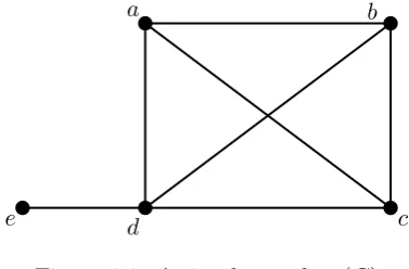
Example 4.8. LetM1 be the four-point line on the ground set{1,2,3,4}and letM2 be
the matroid on the ground set{5,6,7,8}with circuitsC={{5,6,7},{5,6,8},{7,8}}(see
Figure 4.1). Then an independent set of M1⊕M2 is formed by taking the union of an
independent set in M1 with one from M2. For example, the set{1,3,5} is independent
in M1 ⊕M2. Note, that r(M1 ⊕M2) = r(M1) +r(M2) = 2 + 2 = 4, since a basis for
M1⊕M2 is simply the union of a basis ofM1 with a basis of M2.
1 2 3 4
M1
5 6 7 8
M2
1 2
3 4
5 6
78
M1⊕M2
Figure 4.1: The direct sumM1⊕M2.
In our attempt to construct regular round matroids using Seymour’s
Decompo-sition Theorem, we are going to consider the direct sum and show that we can not obtain
a round matroid by using this operation.
Proof. Let M1 and M2 be matroids with the sets of cocircuits C∗(M1) and C∗(M2) re-spectively. Then by Proposition 4.8(v), C∗(M1⊕M2) = C∗(M1)∪ C∗(M2). Therefore, matroid M =M1⊕M2 has disjoint cocircuits and, thus, is not round.
In the next section we will investigate the operation of 2-sum.
4.4
The Operation of 2-sum
The operation of 2-sum allows one to join matroids with exactly one common
element. Before we define the operation of 2-sum for all matroids, we are going to see
how we can apply this operation to graphs and cycle matroids.
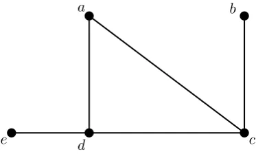
Example 4.10. Consider graphs G1 and G2 shown on Figure 4.2 (a) and (b). If we
assume that M(G1) and M(G2) are the corresponding cycle matroids, then the graphs
in (c) and (d) are isomorphic to the matroidsP(M(G1), M(G2)) andS(M(G1), M(G2)),
the parallel connection and series connection of M(G1) and M(G2) with respect to the
basepoint p. Observe, that the graph in (e) can be obtained both from the graph in (c)
by contractingpand from the graph in (d) by deletingp. The cycle matroid of this graph
p
(a) G1
p
(b)G2
p
(c)
p
(d)
(e)
Figure 4.2: The parallel and series connections and 2-sum of graphs.
Moreover, the graph in (e) can also be obtained directly from G1 and G2 by
identifying the edges labeled p and then deleting the identified edge. We call a graph
obtained in this way a 2-sum ofG1 andG2. To ensure that this operation is well-defined,
we insist that if the edge p is a loop in one of G1 and G2, then it is a loop in the other.
By analogy with the above operation for graphs, there is the following definition
for matroids.
Definition 4.11 (2-sum of matoirds). Let M and N be matroids, each with at least two elements. Let E(M) ∩E(N) = {p} ad suppose that neither M and N has {p}
as a separator. Then the 2-sum M ⊕2N of M and N is S(M, N)/p or, equivalently,
P(M, N)\p.
ClearlyM⊕2N =N⊕2M. The elementpis called thebasepoint of the 2-sum,
and M and N are called the parts of the 2-sum. Note that sometimes, to ensure that the
2-sum has more elements than its parts, the definition of M⊕2N requires that each of
The above definition of the 2-sum and information on representable matroids
found in Section 2.3 will help us to prove the next result.
Proposition 4.12. The 2-sum of two regular matroids is never round.
Proof. LetM1 andM2 be regular matroids whose ground sets meet in a single elementp.
Let matroids M1 and M2 be represented by binary matrices A1 and A2, respectively, in
row echelon form. Then the matrix in Figure 4.3 is a totally unimodular representation
for a parallel connection P(M1, M2) with respect to p.
E(M1)−p p E(M2)−p
0 0
A1 ... 0
0 0 1 0 0
0 ... A2
0 0
Figure 4.3: Matrix representation of P(M1, M2).
Therefore,M1⊕2M2=P(M1, M2)\pcan be represented by a matrix in Figure
4.4.
E(M1)−p E(M2)−p
A1 0
0 A2
Figure 4.4: Representation forM1⊕2M2 =P(M, N)\p.
To show that matroidM =M1⊕2M2 is not round, we will look at its cocircuits.
cocircuit, viewed as the compliment of a hyperplane, can be found in a regular matroid
by fixing a row in the corresponding matrix and looking at all the columns with
non-zero entries in that row. The set of such columns corresponds to a cocircuit. Applying
this technique to the representation for M1⊕2M2 shown in Figure 4.4, we can see that
cocircuits which originated from matroidM1 do not intersect cocircuits which originated
from matroid M2. Therefore, matroidM =M1⊕2M2 is not round.
In the next section we will investigate the operation of 3-sum.
4.5
The Operation of 3-sum
The operation of 3-sum of two regular matroids is analogous to the operation
of 3-sum of two graph. If G1 and G2 are graphs, each containing a 3-cycle, then to
obtain their 3-sum, one first pairs the vertices of the chosen 3-cycle of G1 with distinct
vertices of the chosen 3-cycle in G2. The paired vertices are then identified, as are the
corresponding pairs of edges. Finally, all identified edges are deleted. This process is
illustrated in Figure 4.5 below.
1
2
3
G1
20 10
30
G2
2 = 20 1 = 10
3 = 30
In order to extend the operation of 3-sum from graphs to matroids, we first
introduce the operation defined in Lemma 4.13 below.
Lemma 4.13. Let M1 andM2 be binary matroids andE =E(M1)4E(M2). Then there is a matroid M14M2 with ground set E whose set of circuits consists of the minimal
non-empty subsets of E of the form X14X2, where Xi is a disjoint union of circuits of
Mi. Furthermore, if A is a matrix over GF(2) whose columns are indexed by the elements
of E(M1)∪E(M2) and whose rows consist of the incidence vectors of all the circuits of
M1 and all the circuits of M2, then
M14M2 = (M[A]∗)\(E(M1)∩E(M2)).
Now suppose that the ground sets of binary matroidsM1 and M2 meet in a set
T that is a triangle to both. When both |E(M1)| and |E(M2)| exceed six and neither
M1 norM2 has a cocircuit contained inT, we callM14M2 the3-sum,M1⊕3M2, ofM1
and M2. The next two lemmas outline key properties of 3-sums. Lemma 4.14 describes
circuits in a 3-sum.
Lemma 4.14. Let M1 andM2 be binary matroids such thatE(M1)∩E(M2) =T, where T is a triangle of bothM1 andM2. ThenC(M14M2)is the union of C(M1/T),C(M2/T),
and the collection of minimal sets of the form C14C2 where Ci is a circuit of Mi such
that C1∩T =C2∩T and the last set has exactly one element.
Another way to define the operation of 3-sum for binary matroids is in terms of
generalized parallel connection.
Lemma 4.15. Let M1 and M2 be binary matroids and E(M1)∩E(M2) = T. Suppose
that T is a 3-circuit of both M1 and M2, that |E(M1)| and |E(M2)| exceed six, and that
T does not contain a cocircuit of M1 andM2. Then
M1⊕3M2 =PT(M1, M2)/T.
MatroidPT(M1, M2)/T is also called themodular sum ofM1 and M2. Viewing
the operation of 3-sum in terms of generalized parallel connection allows one to construct
its matrix representation. The process was described and proved by a matroid theorist,
Lemma 4.16. Let PT(M1, M2) be the generalized parallel connection of M1(E1∪˙T) and
M2(E2∪˙T). Then PT(M1, M2) isF-representable if and only if there exists a
representa-tion N1 for M1 and N2 for M2 and there is a linear transformation that is nonsingular
on N1 taking the columns indexed by T in N1 to those indexed by T in N2.
In this case,T has a common representation DT in representations for M1 and
M2, respectively, and PT(M1, M2) is represented by
N=
D2 0 0
D1 DT D
0
1
0 0 D02
and
D2 0
D1 D
0
1
0 D02
represent the associated modular sum,
where
N1=
D2 0
D1 DT
represents M1,
N2=
DT D
0
1
0 D02,
represents M2.
We will use the above result to show that the 3-sum of two regular matroids can
not be round.
Proposition 4.17. The 3-sum of two regular matroids is never round.
Proof. Let M1 and M2 be regular matroids and E(M1)∩E(M2) = T. Suppose thatT
is a 3-circuit of both M1 and M2, that |E(M1)| and |E(M2)| exceeds six, and that T
does not contain a cocircuit of M1 and M2. Since regular matroids can be represented
overGF(2), thenM1⊕3M2 =PT(M1, M2)/T. Let matrices A1 and A2 in Figure 4.6 be
representations of M1 and M2 with DT being a representation of a 3-circuit T in both