https://doi.org/10.5194/jsss-8-105-2019
© Author(s) 2019. This work is distributed under the Creative Commons Attribution 4.0 License.
SimOptDevice: a library for virtual optical experiments
Reyko Schachtschneider1, Manuel Stavridis1, Ines Fortmeier2, Michael Schulz2, and Clemens Elster1 1Physikalisch-Technische Bundesanstalt, Abbestr. 2–12, 10587 Berlin, Germany
2Physikalisch-Technische Bundesanstalt, Bundesallee 100, 38116 Braunschweig, Germany
Correspondence:Reyko Schachtschneider ([email protected])
Received: 28 August 2018 – Revised: 12 February 2019 – Accepted: 13 February 2019 – Published: 27 February 2019
Abstract. Virtual experiments have become an indispensable tool for the design and the accuracy assessment of novel measurement procedures and instruments. Virtual experiments are particularly relevant in modern op-tics due to its challenging demands for highly accurate measurements. This paper introduces SimOptDevice, a flexible library for opto-mechanical virtual experiments. After describing the scope and general structure of the library, its underlying mathematical tools used for solving the related numerical tasks are described. Finally, the application of SimOptDevice to a recent interferometric measurement procedure is presented.
Copyright statement. The author’s copyright for this publication is transferred to the Physikalisch-Technische Bundesanstalt (PTB).
1 Introduction
Following the advance of technology and the demand for highly accurate measurements, optical instruments and ex-periments have become very complex in recent years. In ad-dition, sophisticated data analysis has become an important part of modern optical measurement devices. To ensure that a measurement principle is fit for its purpose, it is beneficial to first test it in a virtual environment prior to building the physical setup. That way, experimenters can save time and costs in the development of novel procedures. Furthermore, virtual experiments are often essential for the assessment of accuracies that can be reached.
For these reasons, virtual experiments have become an important tool in optics. Examples of applications are non-null interferometer calibration (Hao et al., 2016), valida-tion of new data analysis techniques (Shen et al., 2015), absolute flatness measurements of optical surfaces (Bouillet and Morin, 2014), and accuracy evaluations in interferomet-ric measurements (Wiegmann et al., 2011) or deflectometinterferomet-ric flatness measurements (Schulz et al., 2010). Virtual exper-iments have become essential also in many other scientific fields, e.g. simulations of X-ray optics experiments (Knud-sen et al., 2013), neutron scattering (Lieutenant et al., 2004), uncertainty assessment in computer tomography (Hiller and
Reindl, 2012) or coordinate measurement machines (Heißel-mann et al., 2017; Trenk et al., 2004), cross-borehole imag-ing (Donato and Crocco, 2015), or error quantification of CNC milling machines (Soori et al., 2013).
The Physikalisch-Technische Bundesanstalt (PTB) has de-veloped the SimOptDevice software library for optical vir-tual experiments. SimOptDevice is a flexible library im-plemented in MATLAB® (MATLAB, 2018) that covers a large range of applications. It facilitates the design of ex-periments and allows one to develop and test measurement procedures. Furthermore, SimOptDevice is used to optimize existing measurement procedures with respect to measure-ment time and uncertainty. The latter is particularly relevant for PTB, which aims at measurements at the highest level of accuracy. Successful examples using SimOptDevice in-clude accuracy evaluation of interferometric measurements of a synchrotron mirror (Wiegmann et al., 2011), develop-ment of a deflectometric flatness reference at PTB (Schulz et al., 2010; Ehret et al., 2012), and accuracy tests for multi-spectral imaging systems (Dierl et al., 2018).
through a series of optical elements. It considers nested scan-ning stages accounting for translations and rotations, and supports the use of various sensors such as cameras. SimOpt-Device is based on the application of ray optics.
The basic principle of SimOptDevice is a system of hier-archical coordinate systems, combined with ray tracing rou-tines. Within each coordinate system, optical elements can be placed. A related local coordinate system is assigned to each considered optical element, along with a superordinate coor-dinate system relative to which the local coorcoor-dinate system is defined. In this way, a tree structure of coordinate systems is built. Each local coordinate system can undergo individ-ual rotations and translations with respect to its superordinate system. The coordinates of each element can be transformed into any of the other employed coordinate systems. Those transformations are made simple by using homogeneous co-ordinates which are introduced in Sect. 3.1.
The power of SimOptDevice lies in tracing rays and per-forming ray aiming accurately and efficiently according to the laws of refraction and reflection while being in control of all optimization parameters and the applied algorithms. Us-ing the library for our experiments, we view and verify all intermediate results, which is very helpful for tuning the al-gorithms for each specific problem. Whereas ray tracing fol-lows a ray through the optical system when start point and di-rection are given, ray aiming seeks the path through the sys-tem for given start and end points. The latter is a highly non-linear optimization problem. Details are described in Sect. 3. The accurate modelling of all elements of a measurement setup is another advantage of SimOptDevice. This includes not only optical elements like lenses, mirrors and sensors but also linear stages and rotary tables. Ensembles of elements can be saved and reused in other virtual experiments.
During development, the software has been successfully checked against ray tracing results obtained by ZEMAX. This included comparisons of optical path lengths and of points reached by ray tracing. The differences were in the sub-nanometre range.
3 Mathematical methods
3.1 Coordinate transformations
One key feature of SimOptDevice is its easy way to trans-form coordinates from any local system to any other
coordi-With this coordinate definition, a translation or rotation is represented by a 4×4 matrix:
Translation:
1 0 0 1x
0 1 0 1y
0 0 1 1z
0 0 0 1
,
Rotation aboutxaxis:
1 0 0 0
0 cosθ −sinθ 0 0 sinθ cosθ 0
0 0 0 1
.
Rotations about the other axes are defined analogously. The composition of several homogeneous transformations H1, H2, . . . ,HNis equal to a single homogeneous transformation
H=HN·HN−1·. . .·H2·H1. (1) Using Eq. (1), the translation and rotation of a coordinate sys-tem with respect to its superordinate syssys-tem are represented by a single matrix. The inverse of a homogeneous transfor-mation is represented by the inverse of the corresponding transformation matrix. The aforementioned transformation from one local source systemSa to another destination sys-temSbis performed with the help of a common superordinate systemSc:
Ha→b=H−1b→c·Ha→c. (2) For a more comprehensive introduction to homogeneous co-ordinates, see e.g. Cox et al. (2007) or Hartley and Zisserman (2003).
3.2 Ray tracing
Figure 1.Example of the hierarchical structure of coordinate systems in SimOptDevice.(a)The plot of a coordinate system tree example is shown. The left column lists the element names; the right column shows a sketch of the hierarchical structure of the coordinate systems. (b)The corresponding instrument is illustrated. The position and orientation of each of the instrument’s subsystems are defined with re-spect to the superordinate system through a transformation of homogeneous coordinates. A transformation matrixHcan be computed for transformations from one system to another (see Eq. 2). It is a function of the source system and the destination system (in this example SensorandTopo, respectively). The common superordinate systemTs_Frameis needed for the computation of the transformation matrix (cf. Eq. 2). Subsequently, coordinates of a point in one system can be transformed to any other system by multiplication by the corresponding transformation matrixH.
pTi ,eTi T =fi pi−1,ei−1. (3)
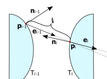
Functionfi entails performing the following steps (cf. Fig. 2 for an illustration):
1. transformation ofpi−1andei−1from systemTi−1toTi,
2. calculation of the ray’s geometrical path lengthli be-tweenTi−1andTi,
3. determination of next intersection pointpi=pi−1+li·
ei−1,
4. calculation of normal vectornionTi inpi, and
5. calculation of the new ray directionei according to the laws of refraction and reflection.
This is classical ray tracing with the particular feature that at each boundary the intersection point and the new direc-tion are calculated in the new local coordinate system. Step 3 is calculated analytically for planes and spherical surfaces and has to be calculated numerically for more complex sur-faces like Zernike sursur-faces, aspheres, or sursur-faces described by a Gauss function. If the ray passesN surfaces, there are N different functionsfi. The last intersection point and ray direction can be expressed as a function of the start point and direction by concatenation of functionsf1tofN:
pTN,eTNT =fN fN−1 . . .f2 f1 p0,e0. . .
=f p0,e0
. (4)
Furthermore, for each crossing of a boundaryTi a Jacobian matrix containing the partial derivatives of the intersection pointpi and the ray directionei with respect to the previous
Figure 2.Schematics of a ray tracing step. Each topographyT has its own coordinate system. The intersection pointpi with topogra-phyTi is computed from the previous intersection pointpi−1and the previous ray directionei−1. Subsequently, the new ray direc-tionei atTi is computed according to the laws of reflection and
refraction.
intersection pointpi−1and the previous ray directionei−1is calculated. It is associated with Eq. (3) and has the following form:
Ji=
∂xi
∂xi−1 ∂xi
∂yi−1 ∂xi
∂xˆi−1 ∂xi
∂yˆi−1 ∂yi
∂xi−1 ∂yi
∂yi−1 ∂yi
∂xˆi−1 ∂yi
∂yˆi−1 ∂xˆi
∂xi−1 ∂xˆi
∂yi−1 ∂xˆi
∂xˆi−1 ∂xˆi
∂yˆi−1 ∂yˆi
∂xi−1 ∂yˆi
∂yi−1 ∂yˆi
∂xˆi−1 ∂yˆi
∂yˆi−1
,
direction. These Jacobian matrices are used extensively when performing the ray aiming. Their usage is explained in more detail in Sect. 3.3. A detailed description of the ray tracing and ray aiming procedures can also be found in Fortmeier (2016, in German).
3.3 Ray aiming
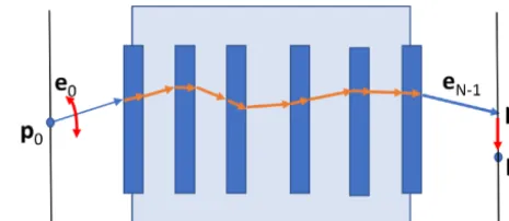
Given a start point p0 and an end point pdestN the task of ray aiming is to find the start directione0fromp0in order to minimize the distance between pN and the desired end pointpdestN (see Fig. 3):
ˆ
e0=argmin e0
pN(e0)−p dest
N
. (6)
where|| · ||denotes the Euclidean norm andpN is reached through application of ray tracing for a chosen start direc-tion e0. For successful ray aiming the resulting norm in Eq. (6) is close to zero. This is usually a highly nonlin-ear problem. It can be solved using one of MATLAB®’s parallel nonlinear solver routines, e.g. lsqnonlin. The latter is a solver for nonlinear least-squares problems in which thetrust-region-reflectiveorLevenberg–Marquardalgorithm can be applied. For better convergence of the solver, the ray tracing Jacobian matrix from Eq. (5) is utilized in this step. The Jacobian matrices calculated during ray tracing are used to update the start directione0when minimizing the distance between pointpNand pointpdestN . Furthermore, SimOptDe-vice delivers the Jacobian matrices for the change in total optical path lengths with respect to changes in a pointpi or a ray directioneifor each surfaceTi(Fortmeier et al., 2014). It is calculated analytically, thereby omitting the computa-tionally expensive extra ray tracing steps for the numerical differentiation. The Jacobian matrices for ray aiming are im-portant in many interferometric applications, e.g. the tilted-wave interferometer (cf. Sect. 4), where the change in the optical path length of a ray is a significant quantity of the experiment.
A requirement for successful ray aiming is that the desti-nation pointpdestN can be reached. Therefore, the valid area on the CCD (or any other final surface) is determined in a preceding step. A ray aiming between the light source and some characteristic points at the smallest aperture in the op-tical system is performed. The final ray directions at the aper-ture are used to trace the rays to the CCD, thereby defining
0 andpdestN of a ray are given. The task is to find the correct start anglee0such that the desired end point is hit. This is achieved by minimizing the distance between pointspNandpdestN , whenpNis reached through application of ray tracing for a chosen start direc-tion,e0.
the area that can be reached by rays from the sources. A ray aiming is regarded as successful if the norm of the difference in Eq. (6) is smaller than 1 nm. Local minima that prevent the algorithm from converging are detected and such rays are masked. Using the Jacobian matrix, the ray aiming usually converges in about four steps. Without the Jacobian matrix this takes approximately 12 to 15 steps, depending on the particular situation.
4 Application example: tilted-wave interferometer
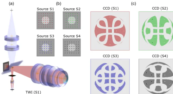
The tilted-wave interferometer (TWI) is an interferometric measurement device for form measurements of asphere (Gar-busi et al., 2008) and freeform surfaces. Figure 4 illustrates the simulation of interferograms for a measurement of an as-phere. For SimOptDevice, the TWI is a particular application example since virtual experiments are not only used for de-signing the instrument and measurement setup, but are also an integrated part of data analysis. More precisely, we use SimOptDevice to obtain a numerical model of the experi-ment in dependence on the unknown form of the asphere or freeform surface under test. The latter is retrieved as the so-lution of a nonlinear inverse problem where in our imple-mentation SimOptDevice constitutes the model. The inverse problem is solved iteratively, which is facilitated through the parallel computing capabilities of SimOptDevice. The non-linear problem is non-linearized with the help of Jacobian matri-ces (Fortmeier et al., 2014). The solution of the inverse prob-lem is found with the MATLAB®routinefsolve. It is possi-ble to use different solver algorithms withfsolve. We typ-ically choose trust-region-dogleg or trust-region-reflective. Trust region algorithms locally approximate the cost function by a quadratic function and progress towards the minimum of this approximation.
Figure 4.Examples from the tilted-wave interferometer (TWI) simulation.(a)Ray paths through the instrument. Source array, reference and test arms, and detector (CCD).(b)The sources of the laser array are switched on in four groups (S1 to S4);(c)simulated interferograms on the CCD for each of the source groups for an asphere example.
have to be characterized very accurately prior to a measure-ment. For this calibration process, well-known test speci-mens (typically spheres) are measured with the TWI (Baer et al., 2014). The numerical model is then updated by adjust-ing the Zernike polynomial parametrization of two reference surfaces in order to account for the remaining discrepancies. SimOptDevice has also been used for uncertainty evalua-tion (Fortmeier et al., 2017) of the TWI and for the explo-ration of new measurement concepts with the TWI (Fort-meier et al., 2016).
5 Conclusions
SimOptDevice is a versatile library for conducting virtual opto-mechanical experiments that has been applied success-fully in several projects and studies. SimOptDevice can model a large number of optical elements and sensors which can be combined flexibly to cover a wide range of experi-mental setups.
We have explained the mathematical concepts within the library. A detailed description of our ray tracing and ray aim-ing procedures and of the determination of Jacobian matri-ces, needed for efficiently solving the nonlinear inverse prob-lems, was given. This will be useful for readers interested in implementing virtual optical experiments. We also conclude that SimOptDevice can be used to simulate very complex opto-mechanical systems.
Data availability. No data sets were used in this article.
Competing interests. The authors declare that they have no con-flict of interest.
Special issue statement. This article is part of the special issue “Sensors and Measurement Systems 2018”. It is a result of the “Sen-soren und Messsysteme 2018, 19. ITG-/GMA-Fachtagung”, Nürn-berg, Germany, from 26 June 2018 to 27 June 2018.
Acknowledgements. The authors sincerely thank the EMPIR organization. The EMPIR is jointly funded by the EMPIR par-ticipating countries within EURAMET and the European Union (15SIB01: FreeFORM).
Edited by: Eric Starke
Reviewed by: two anonymous referees
References
Baer, G., Schindler, J., Pruss, C., Siepmann, J., and Osten, W.: Cal-ibration of a non-null test interferometer for the measurement of aspheres and free-form surfaces, Opt. Express, 22, 31200, https://doi.org/10.1364/OE.22.031200, 2014.
Bouillet, S. and Morin, C.: Method for the absolute measurement of the flatness of the surfaces of optical elements, Google Patents, US Patent App. 14/236,487, 2014.
Cox, D., Little, J., and O’Shea, D.: Ideals, Varieties, and Algo-rithms: An Introduction to Computational and Commutative Al-gebra, 3rd Edn., Springer, New York, 2007.
Dierl, M., Eckhard, T., Frei, B., Klammer, M., Eichstädt, S., and Elster, C.: Novel accuracy test for multispectral imaging systems based on1E measurements, J. Eur. Opt. Soc.-Rapid Publ., 14, 1, https://doi.org/10.1186/s41476-017-0069-1, 2018.
Fortmeier, I., Stavridis, M., Wiegmann, A., Schulz, M., Osten, W., and Elster, C.: Evaluation of absolute form measurements using a tilted-wave interferometer, Opt. Express, 24, 3393, https://doi.org/10.1364/OE.24.003393, 2016.
Fortmeier, I., Stavridis, M., Elster, C., and Schulz, M.: Steps towards traceability for an asphere interferome-ter, in: Optical Measurement Systems for Industrial In-spection X, Proc. SPIE, 10329, 1032939-1–1032939-9, https://doi.org/10.1117/12.2269122, 2017.
Garbusi, E., Pruss, C., and Osten, W.: Interferometer for pre-cise and flexible asphere testing, Opt. Lett., 33, 2973, https://doi.org/10.1364/OL.33.002973, 2008.
Hao, Q., Wang, S., Hu, Y., Cheng, H., Chen, M., and Li, T.: Vir-tual interferometer calibration method of a non-null interferom-eter for freeform surface measurement, Appl. Optics, 55, 9992– 10001, https://doi.org/10.1364/AO.55.009992, 2016.
Hartley, R. and Zisserman, A.: Multiple View Geometry in com-puter vision, Cambridge University Press, Cambridge, 2003. Heißelmann, D., Franke, M., Rost, K., Wendt, K., Kistner, T., and
Schwehn, C.: Determination of measurement uncertainty by sim-ulation, arXiv:1707.01091 [physics], available at: http://arxiv. org/abs/1707.01091 (last access: February 2019), 2017. Hiller, J. and Reindl, L. M.: A computer simulation platform
for the estimation of measurement uncertainties in dimensional X-ray computed tomography, Measurement, 45, 2166–2182, https://doi.org/10.1016/j.measurement.2012.05.030, 2012.
https://doi.org/10.1117/12.562814, 2004.
MATLAB: release R2018b, The Mathworks, Inc., Natwick, MA, 2018.
Schulz, M., Ehret, G., Stavridis, M., and Elster, C.: Concept, de-sign and capability analysis of the new Deflectometric Flatness Reference at PTB, Nucl. Instrum. Meth. Phys. Res. Sect. A, 616, 134–139, https://doi.org/10.1016/j.nima.2009.10.108, 2010. Shen, H., Zhu, R., and Li, J.: Assessment of optical
freeform surface error in tilted-wave-interferometer by combining computer-generated wave method and re-trace errors elimination algorithm, Opt. Eng., 54, 074105, https://doi.org/10.1117/1.OE.54.7.074105, 2015.
Soori, M., Arezoo, B., and Habibi, M.: Dimensional and geo-metrical errors of three-axis CNC milling machines in a vir-tual machining system, Computer-Aided Design, 45, 1306–1313, https://doi.org/10.1016/j.cad.2013.06.002, 2013.
Trenk, M., Franke, M., and Schwenke, H.: The “Virtual CMM” a software tool for uncertainty evaluation – practical applica-tion in an accredited calibraapplica-tion lab, in: Proc. of ASPE: Uncer-tainty Analysis in Measurement and Design, American Society for Presicion Engineering, Rayleigh, NC, USA, 2004.