GENERALISED MODEL BASED CONFIDENCE INTERVALS IN TWO STAGE CLUSTER SAMPLING

in Two Stage Cluster Sampling

Christopher Ouma Onyango

Center for Mathematics Strathmore University Nairobi, Kenya

[email protected]

Romanus Odhiambo Otieno

Department of Statistics Jomo Kenyatta University Nairobi, Kenya

[email protected]

George Otieno Orwa

Department of Statistics Jomo Kenyatta University Nairobi, Kenya

[email protected]

Abstract

Chambers and Dorfman (2002) constructed bootstrap confidence intervals in model based estimation for finite population totals assuming that auxiliary values are available throughout a target population and that the auxiliary values are independent. They also assumed that the cluster sizes are known throughout the target population. We now extend to two stage sampling in which the cluster sizes are known only for the sampled clusters, and we therefore predict the unobserved part of the population total. Jan and Elinor (2008) have done similar work, but unlike them, we use a general model, in which the auxiliary values X_i are not necessarily independent. We demonstrate that the asymptotic properties of our proposed estimator and its coverage rates are better than those constructed under the model assisted local polynomial regression model.

Keywords and Phrases: Model Based Surveys, Bootstrapping, Two Stage Sampling

AMS 2000 subject classifications. Primary 60K35; Secondary 60K35.

1. Introduction

1.1 Background

population of N identifiable units, Y denotes a survey variable having population values Yi, (i= 1, 2, 3,...,N) and Xto denote an auxiliary variable with

corresponding population valuesXi, (i= 1, 2, 3,...,N). If the values , ( 1, 2, 3,..., )

i

X i= N are all known but the characteristic values Y_i, (i= 1, 2,3,...,N)

are known only for a Sample, say s, of n≤ Nof the population elements, one way of characterizing the sample selection of the survey variable is to assume that for every unit on the sampling frame, a new variable, say S_i takes a value equivalent to the number of times which that particular population unit’s value is observed. The distribution of these values defines the design of the sample survey.

Once the sample has been chosen, the values ( ,Y ii ∈s) are known. Now, let the

distribution of S_i depend on the known population values of X and suppose that one wishes to use the sample values together with the known values of X to

make an inference about the unknown but finite population total 1 N

i i

T Y

=

=

∑

ofY. A

major concern in model based approach to statistical survey inference has been finding robust estimators for the population parameters under model misspecifications.

1.2 Outline of the paper

This paper is organised as follows. In Subsections 1.3, 1.4, 1.5, 1.6, we give a brief highlight on model based estimation, the local polynomial estimation, confidence intervals, and two stage cluster sampling respectively, in each case, pointing out some gaps that our proposed estimator attempts to fill. In Section 2, we propose an estimator for the finite population total and suggest a bootstrap confidence interval for it in Section 3. In Section 4, we derive the properties of our proposed estimator. We conclude this paper in Section 5 with a simulation experiment and some discussions.

1.3 Review of model based estimation

1.4 Review of the local polynomial estimation

Dorfman (1992) considered a non-parametric regression model for estimating population totals in finite populations. He proposed a non-parametric regression based estimator for the population total. To develop the estimator, he assumed that the population values were generated by a model defined as

( )

i i i

Y = m x + e (1.1)

where i=1, 2, 3,...,N , m

( )

. is a smooth function and e_i is an independent random variable with mean zero and constant variance. The non-parametric population total estimator due to Dorfman (1992) is defined as

( )

D _{i i}

i s i s

T Y m x

∧ ∧

∈ ∈

=

∑ ∑

+ (1.2)

where

( )

i i i i i s

m x w x y

∧

∈

=

∑

and _{i i b}

(

_i

)

_b

(

_i

)

s

w x =k x −x

∑

k x −x is the weight associated

with the ith unit of the sample. Further, k u

( )

is a symmetric density function, b a scaling factor and

( )

1

(

)

/

b

k u =b k u b− . In his empirical study, Dorfman (1992)

illustrated that the estimator TD

∧

performs better when compared to the corresponding design based and linear regression estimators. These results were also confirmed by Cheng (1994) who applied non-parametric regression in estimating population parameters under conditions of missing data. Breidt and Opsomer (2000), also assumed model 1.1 and developed a new class of model-assisted non parametric regression estimators for the population total, based on local polynomial smoothing, a kernel method. Their estimator is defined as

i i

OB i

i s i i s

y m

T m

π

∧

∧ ∧

∈ ∈

−

=

∑

+

∑

(1.3)

where

1, 2, 3,...,

i= N, π_i = pr i

(

∈s

)

, mi w y_{si s}

∧

=

and si i j 1 ,

j

x x

k

w diag j s

h h bπ

  −  

=     ∈

   

  with h denoting the bandwidth. In their

simulation study, TOB

∧

performs better than the Horvitz-Thompson estimator defined as

i HT

i s i

Y T

π

∧

∈

=

∑

(1.4)

cluster totals with weights that are calibrated to known control totals. They indicated that the local polynomial regression estimators are constructed by modeling the M points

(

x t_i, _i

)

as a realization from an infinite super population model ζ in which

( )

i i i

t =µ x +e (1.5)

where ei ~ N

(

0,var

( )

x

)

, µ

( )

x is a smooth function of x and var

( )

x is also

smooth and strictly positive. Their estimator is defined as

i _i

y _i

i s i s i

t

t µ µ

π

∧ ∧

∧ ∧

∈ ∈

−

=

∑

+

∑

(1.6)

where

(

)

1

' ' '

s

i e X W Xi si si si X W tsi si

µ∧ = − _ ∧ _

  (1.7)

In the equation 1.7,

1

i j si

m m j

x x

k

w diag

h h bπ

  −  

=    

   

 , 1,

(

) (

,...,

)

q

si j i j i

j s

X x x x x

∈

 

=_ − − _

and e_irepresents the first column of the identity matrix X_si. In their simulation results they concluded that the estimator 1.6 is more efficient than the Horvitz-Thompson and the linear regression estimators when the mean function of the super population model is non linear while being nearly as efficient when the model is linear.

Recently, Jan and Elinor (2008) considered the problem of estimating the population total in two-stage cluster sampling when cluster sizes are known only for the sampled clusters, making use of a population model arising from a variance component model. They considered the application of predictive likelihood technique in estimation of the unknown part of the population total

∑∑

= =

= N

i m j

ij

i

y T

1 1

(1.8)

where Nis the number of primary sampling units or clusters and each cluster consists of m_i units which are only known for the sampled clusters, yij is the value of the variable of interest for unit jof the ith cluster. They assumed the population model defined by the equations

( )

( )

2

( )

(

)

, var var , cov 0

i i i i i j

E M =βx M =σ x M M = (1.9)

( )

( )

2

( )

2

, var , cov

ij ij ij ik

E Y =µ Y =τ Y Y =ρτ (1.10)

in cases where j≠k and ρ≥0. To predict the unobserved value of Z in the estimate of the population total T given by

1 1

i

M N

ij i j

T Y Z

∧ ∧

= =

they developed a partial likelihood for Z, L z y

( )

, from the generalized joint likelihood for the unknown quantities zand θgiven by

( )

,

( )

,

L z y = f_θ z y (1.12)

They applied the design based Horvitz-Thompson estimator of population total,

i i HT

i s

o i

m y x

T

n x

∧

∈

=

∑

(1.13)

where n₀, represents the number of the primary sampling units selected in first stages and the model. In their simulation, they considered three coverage measures ofZ; the model based over the joint distribution of YandZ, the design based over the sampling design, and regarding the total sample as a stochastic variable. They concluded that for a small number and the unconditional coverage no of sampled clusters, the three intervals differ significantly, but for large n0, the three intervals are practically identical.

Further, a comprehensive simulation study of the model based and the design coverage properties of the prediction intervals indicate that for large sample sizes, the coverage measures achieve approximately the nominal level 1−α and are slightly less than 1−αfor moderately large samples and for small sample sizes, the coverage measures are about1 2− α, being raised to 1−α for a modified interval based on

0 2

n

t ₋ distribution. We note that the models 1.9 and 1.10 assume that the regression line passes through the origin and that the auxiliary values X_i are considered independent. The questions raised in subsection 1.3 therefore remain unanswered.

1.5 Review of confidence intervals in survey sampling

Confidence intervals are usually constructed around point estimators in order to provide a properly scaled measure of uncertainty associated with the estimator. The conventional method is based on the assumption that the sample size is large enough for the Central Limit Theorem to hold. This is however not always true in practice.

As a consequence Do and Kokic (2001), Chambers and Dorfman (2002) applied the bootstrap method to develop model based confidence intervals to address situations where the sample sizes are not large. They also proposed modifications of the procedure to account for misspecifications in a working model. They further noted that there is greater efficiency in using of successive model refinements and estimators obtained using the bootstrap approach as opposed to their competing estimators. However, the evidence of the extended simulation study on the beef population showed that the achievement of the research did not precisely attain its goal. They therefore recommended the construction of sounder confidence intervals using the bootstrap approach. Ouma and Wafula (2005) suggested the use of a general super population model

( )

i i i

Y m x e

∧ ∧

where i=1, 2, 3,...,N, m

( )

. is a smooth function, e_i is an independent random variable with mean zero and constant variance. They used a bandwidth of 1.5 and simple random sampling with replacement to generate the values of survey variableY. In their empirical study, they established that their coverage rates were higher compared to that of Chambers and Dorfman (2002). We now extend this to two stage cluster sampling.

1.6 Review of two stage cluster sampling

Let U be a finite population of N primary sampling units psu_s or clusters labeled1,2,..,N, U =1, 2,...,N where N is a known number,M_i, i=1,2,..,N be the number of secondary sampling units ssu_s in the th

i psu. Let y _ij i=1,2,..,N, i

M

j=1,2,.., be the value of the response variable Y for the ssu j belonging to thepsu i. In the previous works, an assumption has been made that the element specific auxiliary data '

,

ij

x i=1,2,..,N, j=1,2,..,M_i are known for all clusters and population elements, respectively.

For our case, we assume that the cluster sizes are known only for the sampled clusters and therefore the survey values y_ij, i=1,2,..,N, j=1,2,..,M_i are generated using the model

ij ij ij m x e

Y

^ ^ ^

)

( +

= (1.15)

with i=1,2,..,N j=1,2,..,M_i.

2. Proposed Estimator for population total.

Jan and Elinor [6] used the model 1.15 to define the population total as

∑∑

= =

= N

i m j

ij

i

y T

1 1

(2.1)

where N is the number of primary sampling units or clusters and each cluster consists of m_i units which are only known for the sampled clusters, y_ij is the value of the variable of interest for unit j of the th

i cluster. Referring to the same model 1.15 we may write that

∑ ∑

∑∑

= = + = =

+

= N

i M

m j

ij N

i m j

ij

i i

y y

T

1 1

^

1 1

^ ^

Z Y

s i j s

ij

i

+

=

∑∑

∈ ∈

(2.2)(((

ij

y ,i=1,2,..,N, j=1,2,..,M_i. Therefore the estimate of the population total is given by

( )

∑ ∑

∑∑

= = + = =     ₊ + = N i M m j ij ij N i m j ij i i i e x m y T 1 1 ^ ^ 1 1 ^ (2.3)

3. Proposed Bootstrap Confidence Interval

Under the model based approach, the sampling distribution of the estimator corresponds to the distribution of possible alternative point estimates that could arise given the selection of the same sample Sfrom populations similar to the actual underlying population of the observed data. To construct a confidence interval for Tthat reflects the actual finite sample and finite population

characteristics of the distribution of ^

T we estimate such a distribution from the sample data. For our case, we make use the sample data and the working model 1.15 to generate a sequence of alternative realizations of Yusing non parametric estimates ofm(xij). Let

* ij

Y be an estimator of the values of Y, where ^

*

(

)

ij ij ij

Y

m x

e

∧

=

+

(3.1)

In equation 3.1, e_ij is selected via two stage cluster sampling with replacement fromeij:i=1, 2... ,n j=1, 2,..mi.

Having obtained the bootstrap population, the bootstrap version 1* ^

T of 1

^

T , using the same sample as the parent sample, is calculated. The process is then

repeated a large number, B, of times to obtain * ^ * 2 ^ * 1 ^ ,....

, i iB

i T T

T . Then the bootstrap confidence interval is obtained using

( )

_    _      − 2 1 , 2 * * α α Q Q

where

Q

*

(

p

)

is the th

p – quantile of bootstrap distribution.

4. Properties of the proposed estimator and resulting confidence interval

4.1 Unbiasedness of the model

Considering the model 1.15 we may write that

)

(

^

ij ij

ij

Y

m

x

e

=

−

(4.1)

and = ) ( * ij x W                       − +               − − i ij r m n n m n m W 2 1 2 1 2 1 1 1

where m is the bootstrap sample size, r_i is the number of times the

i

th primary sampling unit is selected, x_ij is the th

j observation made from the th

i cluster, and

) (xij

W is the initial sampling weight of secondary sampling unit equal to the inverse of its selection probability, that is;

) (xij

W =

ij π

1

(4.3)

with i=1,2,..,n; j=1,2,..,n_i.

However there is considerable benefit and little loss in choosingm=n−1. Rao and Wu (1998)

Therefore, = ) ( * ij x W 1 2 1 1 i ij n r n

π  −  (4.4)

n

i=1,2,.., ; j=1,2,..,m_i, and

(

^

)

^

) ( ij ij

ij E Y m x

e

E = −

     _(4.5) So

∑

∈ = s j i ij ij

ij W x Y

x m , ^ ) ( * ) ( (4.6)

(i=1,2,..,n, j=1,2,..,n_i) yielding

      ^_{( )} ij x m

E =

1 2

1

ij i i j ij

Y n

E r

n ≠ π

 

  _{ }

 ₋ 

 

∑

_ _ (4.7)

Now, let the initial sampling weight of secondary sampling units

ij ij x W π 1 )

( = be

the kernel based weights. Then we have

(

)

(

)

∑

− − = ik ij b ik ij b ij x x K x x K x

W( ) (4.8)

with

∑

( )=1 ∈s

ij ij

x

w , further, bbeing a scaling factor, K_b(u)=b−1K

( )

u/b and k(u) is a symmetric density function which is such that ∀u∈ℜwith the symbols bearing their usual meanings, then

(a)

∫

( )

∂ =1 ∞

∞ −

u u

k ,(b)

∫

( )

∂ <∞

∞ ∞ − u u k2

, (c)

∫

( )

∂ <∞

∞ ∞ − u u k

u3 2

and (d) k

( ) ( )

u =k −u

Therefore,

^

( )

_ij

(

_ij

)

[ (

_ij

)]

E e

m x

E m x

∧

But as b→0 andnb→∞, ( ) ( )

^

ij ij m x

x

m → meaning that

E e

ij

0

∧

  =

 

 

which is the

mean of e_ij

∧

in model 1.15, completing the proof that the proposed model is unbiased.

4.2 Asymptotic variance of the error term

From subsection 4.1, it follows that 2

^ ^

ij _ij

Var e _{ }=E e _{ }

    (4.10)

Therefore 2 ^ ^     =     ij ij E e

e

Var =

2 ^

)

(







 −

Y

ij

m

x

ij

E

= 2 ^ ^ 2

)

(

)

(

2









+

−

ij ij ij

ij

EY

m

x

E

m

x

EY

(4.11)

which leads to

2

) (e_ij

E =

(

)

(

)

^ 2

ij

ij

Var

m

x

x

+

σ

(4.12) But    ^_{( )} ij x m Var = 1 2 1 1

(

1)

1

ij ik ij i s

x

x

n

Var

n

b k

Y

n

b

− − ∈









−











−











−











∑



1 ^

)

(

−













ij s

x

d

(4.13)

where

( )

(

)

1

1

s ij

b ij ik

d x

k x x

− ∧   =  

∑

₋    ^_{( )} ij x m Var = 2 2 2

(

1)

(

)

1

ij ik ij i s

x

x

n

n

b k

x

n

b

σ

− − ∈

−









−







−







∑





2 ^

)

(

−













ij s

x

d

(4.14)

But 2 ^

)

(

−









ij s

x

d

= 2

)

(

−









ij s

x

d

























−

+

+

−

− −2

1 2 1 3 // 2 2

)

1

(

)

(

)

(

1

k

d

x

O

b

n

b

x

d

b

ij s ij s (4.15) and

)

(

_ij ik ij

x

b

x

x

k

σ









−

=

(

)

(

)

(

2

)

1 3

b

b

O

x

d

x

b

σ

ij s ij

+

+

(4.16)

So using equations 4.15 and 4.16 in equation 4.14 we have that

^

( ij)

var m x =

∑

≠ ∈ − −









−

−













−

k i s i ij ik ij

x

b

x

x

k

b

n

n

n

)

(

)

1

(

1

2 2 2 2

σ

(

^

)

2

−













ij s

x

Next we obtain the asymptotic expansion of ^

( ij)

var m x using the following

theorem as a basis.

Theorem

Let k(u) be a symmetric density function with

0 )

( =

∫

uk u du andk₂ u k u du2

0

=

∫

( ) > . Assume that n and N increase together such

that →π

N n

with0<π <1. If further the sampled and non sampled values of x

are in the interval

[ ]

c,d and are generated by densities d_s andd_p−s respectively, both bounded away from zero on

[ ]

c,d and with continuous second derivatives, and if for any expression of Z, it can be shown explicitly that

[

Z/U

]

A(U) O(B)

E = + andVar

[

Z/U

]

=O(C), then

  

 + +

= 2

1

)

(U O B C

A

Z _p .

Using this theorem, we may write equation 4.17 as

^

(

_ij

)

var m x

=

(

)

1 1

1 2 ₂ 2

(

1)

(

)

1

1

ij

n

n

x

O

n

b

n

σ

− −

−















 −

+

−











−



















(4.18)

which reduces to

^

(

_ij

)

var m x

=

(

)

(

)

1 1

2 ₂ 2

2

(

)

1

1

ij

n

x

O

n

b

n

σ

− −











+

−











−













(4.19)

and noting that as the number,

m

_i

=

n

of the second stage samples tends to be large,

n

−

1

≅

n

so that we have

^

(

_ij

)

var m x

=

( )

(

)

(

)

1 3

2 2

1

1

ij

x

O

n

b

n

σ



₋ −



+



−



−





(4.20)

again asnb→∞, 2

^ ( )

( )

1

ij i

x var m x

n

σ

 _{ =}

  ₋

  (4.21)

hence

2 ^

2

(

)

(

)

1

ij

ij _ij

x

var e

x

n

σ

σ

  =

+

 

−

 

(4.22)

which asn→∞, reduces to

^

2

(

)

ij _ij

var e

  =

 

σ

x

4.3 Conditional relative bias of the estimator for the population total

From its definition, the conditional relative bias of using T ∧

as an estimator of T is

   

 

  

 −T T T

E /

^

= E T E

( )

T /T

^

  

 ₋

    

 _(4.24)

In this case, ^

1 1

i

m N

ij i j

T Y

= =

=

∑∑

=

^ ^

1 1

( )

i

M N

ij ij i j m

m x e

= = +

 ₊ 

 

 

∑ ∑

(4.25)

meaning that

( )

_

  



 _

  



 ₋

    

_{T ET T}

E /

^

=

( )

_ij

i j ij i j

ij

ij e E m x e

x m

E − +

  



 ₊

∑ ∑

∑ ∑

^ ^

)

( (4.26)

Using equation 4.9 in equation 4.26, it can be seen that asn→∞ this bias,

( )

_

  



 _

  



 ₋

    

_{T ET T}

E /

^

asymptotically tends to zero.

5. Empirical Study

5.1 Description of the simulation experiment

Simulation experiments were performed in order to compare the performance of the model based regression estimator with that of the model assisted local polynomial regression estimator in two-stage element sampling due to Ji-Yeon et al. (2009).

To obtain the model based estimator for the population total,Xi are generated as independent and identically distributed on uniform (0, 1) random variables. The population consists of 100 clusters. In stage one a sample of n_i =20 clusters is taken which forms the primary sampling units from the total cluster size N_i =100 using simple random sampling with replacement.

In stage two, from each selected clusters, say i,

(

i=1,2,...n_i

)

we select samplem_ij, j=1,2,...50, from j=1,2,...,mk,...1,000 that is the

th

j sample from a fixed selected th

i cluster using simple random sampling with replacement from total M_k=1000 elements. We consider the variable of interestY_ij,

k

k M

m

j=1,2,..., ,..., which are known only for the sample and using the known auxiliary variablesxij, j=1,2,...,Mk we generate the non sample values using the model given in 1.14.

bootstrap population values and the model Y_ij m x_ij eij ^ ^ *

)

( +

= to

obtainy i y i y i y iMk

* 3 * 2 * 1 *

,... ,

, . Further, we let K(u)~U[0,1] so that the model based regression estimator for the population total is given by equation 2.3

where m

( )

x_ij

^

is defined by equation 1.14 and

( )

^

2

~ 0,

ij _ij

e _ σ x _.

This procedure is repeated a large number 1000 of times such that we

have 1* ^

i

T , 2*

^ i

T , 3*

^ i

T ,…, 1000*

^ i

T .We then construct the 95% confidence intervals for

population totalT i,i 1,2,...N

^

* = _{. Similarly, we compute the local polynomial}

estimator for the population total suggested by Ji-Yeon et al. (2009) given in equation 1.6. For each mean function values ofx_ij, each study variabley_ij

(

j=1,2.

)

for m_k values from M_k elements are generated as

( )

2 1

k jk k

ij j jk

M e M

x

y =µ + (5.1)

where, y_jkis the th

k observation made from the _jth _{cluster, and}

( )

(

ij

)

ij N x

e 2

, 0

~ σ .

Using above bootstrap procedure, the bootstrap estimate of the population total

( )

∑

∑

∈

∈ 

 

 −

+ =

s

i i

i i c

i

ij i

m y x

m T

π ^

^ *

(5.2)

is calculated, whereπi =Pr

{ }

i∈s , i j s h

x x k h diag m

ij ik ij

i ∈

    

  

  

 −

= 1 1 , ,

^

π and m x( ij)

∧

is

as defined in equation 1.4. Similarly, we construct the confidence interval for the population total Tand compare performance of the developed model on estimation of Twith that due to Ji-Yeon et al. (2009) on Local Polynomial regression estimation in two-stage sampling.

In computation of the model assisted local polynomial regression estimators, we again adopt a method due to Ji-Yeon et al. (2009). This we do as a means to having a realistic comparative study. We therefore apply the Epanechnikov

kernel

( )

(

2

)

_{{ }1}

1 4 3

≤ Ι −

= u u

u

k and different bandwidths for computation of the Local

5.2 Simulation Results

Table 1 gives the results of Mean Squared Error of the model based MSEmb and the Local Linear Polynomial regression estimator of the population total in two stage cluster sampling.

Table 1: Mean Squared Error (MSE)

Band width LP MB 0.005 0.7845631 1.2684580 0.006 0.7961103 1.7980100 0.007 0.7528211 1.4856560 0.008 0.7523094 1.4641440 0.009 0.7909287 1.3896480 0.010 0.7740691 0.1187740 0.020 0.7615400 0.0846216 0.030 0.7653660 0.0752471 0.040 0.7639690 0.0720307 0.050 0.7621990 0.0672295 0.060 0.7740690 1.1703404 0.070 0.7615400 0.7534386 0.080 0.7551610 0.7534386

It can be seen that at lower bandwidths the MSE for the model based estimators is higher compared to that of the Local Polynomial regression estimator. As the bandwidth increases, the MSEmb drastically reduces and approximately remains low. It is important to note that an increase in the bandwidth does not significantly change the MSE for the Local Polynomial Regression Estimators LPRE. Generally, the Model based estimator is more efficient than the Local polynomial estimators of the totals. Table 2 is a summary of bias for the model based estimator of the population total and the Local Polynomial regression estimator.

Table 2: Summary Results of Bias

The bias for the model based estimator is much lower than those of the Local Polynomial regression estimators. The large bias associated with the Local Polynomial estimators are reflected in the values of its estimators which are much lower than the true simulated population total of 99.5078. This can best be attributed to the choice of the variance. The precision of estimation can be improved by choosing a smaller value of the variance. Table 3 now presents a summary of the estimated population totals for the model based and the Local Polynomial regression estimators in two stage sampling.

Table 3: Summary Results of Estimated Population Totals

Band width LP MB 0.005 60.81535 99.27500 0.006 61.38900 99.01420 0.007 61.49330 99.92000 0.008 60.93400 99.20200 0.009 59.02400 99.32200 0.010 58.64900 97.47400 0.020 60.24100 93.09100 0.030 59.81800 88.08000 0.040 59.34000 83.90000 0.050 59.30700 79.47900 0.060 58.64900 59.49500 0.070 60.24000 59.82600 0.080 59.82400 59.82600

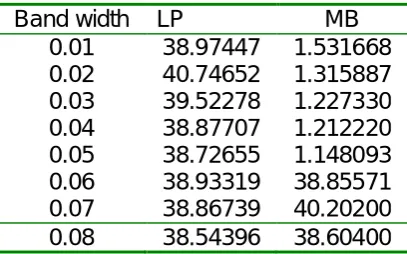
Table 4 now gives the coverage rates of 95 % confidence interval lengths for model based and Local Polynomial Regression models.

Table 4: Confidence Interval Lengths

Band width LP MB 0.01 38.97447 1.531668 0.02 40.74652 1.315887 0.03 39.52278 1.227330 0.04 38.87707 1.212220 0.05 38.72655 1.148093 0.06 38.93319 38.85571 0.07 38.86739 40.20200 0.08 38.54396 38.60400

polynomial regression estimators. The results in general show that the model based approach outperforms the model assisted method at 95% coverage rate. The bias under model based approach is also much lower.

References

1. Breidt, F. and Opsomer, J. (2000). Local polynomial regression estimators in survey sampling. The Annals of Statistics, 28:1026–1053.

2. Chambers, R. and Dorfman, A. (2002). Robust sample survey inference via bootstrapping and bias correction-the case of the ratio estimator. Technical report, Southampton Statistical Sciences Research Institute, University of Southampton.

3. Cheng, P. (1994). Nonparametric estimation of mean functional with data missing at random. Journal of the American Statistical Association, 89: 81–87.

4. Do, K. and Kokic, P. (2001). Bootstrap Variance and confidence interval estimation for model- based surveys. Australia National University.

5. Dorfman, R. (1992). Nonparametric regression for estimating totals in finite population. In Section on Survey Research Methods, Journal of the American Statistical Association, pages 622–625.

6. Jan, F. and Elinor, Y. (2008). Two stage sampling from a predictive point of view when the cluster sizes are unknown. Biometrika, 95 (1): 187–204.

7. Ji-Yeon, K., Breidt, F., and Opsomer, J. (2009). Nonparametric regression estimation of finite population totals under two-stage cluster sampling. Technical report, Department of Statistics, Colorado State University.

8. Ouma, C. and Wafula, C. (2005). Bootstrap confidence interval for model based surveys. East African Journal of Statistics, 1: 14–18.

9. Rao, J. and Wu, C. (1998). Re sampling inference with complex survey data. Journal of the American Statistical Association, 83: 231–241.

10. Smith, T. (1976). The foundations of survey sampling a review. Journal of the Royal Statistical Society, Series A, 139: 183–198.