RESEARCH
Best hits of 11110110111: model-free
selection and parameter-free sensitivity
calculation of spaced seeds
Laurent Noé
*Abstract
Background: Spaced seeds, also named gapped q-grams, gapped k-mers, spaced q-grams, have been proven to be more sensitive than contiguous seeds (contiguous q-grams, contiguous k-mers) in nucleic and amino-acid sequences analysis. Initially proposed to detect sequence similarities and to anchor sequence alignments, spaced seeds have more recently been applied in several alignment-free related methods. Unfortunately, spaced seeds need to be initially designed. This task is known to be time-consuming due to the number of spaced seed candidates. Moreover, it can be altered by a set of arbitrary chosen parameters from the probabilistic alignment models used. In this general context, Dominant seeds have been introduced by Mak and Benson (Bioinformatics 25:302–308, 2009) on the Bernoulli model, in order to reduce the number of spaced seed candidates that are further processed in a parameter-free calcu-lation of the sensitivity.
Results: We expand the scope of work of Mak and Benson on single and multiple seeds by considering the Hit Integration model of Chung and Park (BMC Bioinform 11:31, 2010), demonstrate that the same dominance definition can be applied, and that a parameter-free study can be performed without any significant additional cost. We also consider two new discrete models, namely the Heaviside and the Dirac models, where lossless seeds can be inte-grated. From a theoretical standpoint, we establish a generic framework on all the proposed models, by applying a counting semi-ring to quickly compute large polynomial coefficients needed by the dominance filter. From a practical standpoint, we confirm that dominant seeds reduce the set of, either single seeds to thoroughly analyse, or multiple seeds to store. Moreover, in http://bioinfo.cristal.univ-lille.fr/yass/iedera_dominance, we provide a full list of spaced seeds computed on the four aforementioned models, with one (continuous) parameter left free for each model, and with several (discrete) alignment lengths.
Keywords: Spaced seeds, Dominant seeds, Bernoulli, Hit Integration, Heaviside, Dirac, Counting semi-ring, Polynomial form, DFA
© The Author(s) 2017. This article is distributed under the terms of the Creative Commons Attribution 4.0 International License (http://creativecommons.org/licenses/by/4.0/), which permits unrestricted use, distribution, and reproduction in any medium, provided you give appropriate credit to the original author(s) and the source, provide a link to the Creative Commons license, and indicate if changes were made. The Creative Commons Public Domain Dedication waiver (http://creativecommons.org/ publicdomain/zero/1.0/) applies to the data made available in this article, unless otherwise stated.
Background
Optimized spaced seeds, or best gapped q-grams, have independently been proposed in PatternHunter [3] and by Burkhardt and Karkkainen [4]. The primary objective was either to improve the sensitivity of the heuristic but efficient hit and extend BLAST-like strategy (without
using the neighborhood word principle1), or to increase the selectivity for lossless filters on alignments of size ℓ under a given Hamming distance of k.
Several extensions of the spaced seed model have then been proposed on the two aforementioned problems: vector seeds [5], one gapped q-grams [6] or indel seeds [7, 8], neighbor seeds [9, 10], transition seeds [11–15], mul-tiple seeds [16–19], adaptive seeds [20] and related work on the associated indexes [21–26], just to mention a few.
1 We mention an interesting analysis in [92].
Open Access
*Correspondence: [email protected]
Unfortunately, spaced seeds are known to produce hard problems, both on the seed sensitivity computa-tion [27] or the lossless computation [28], and moreover on the seed design [29]. But the choice of the right seed pattern has a significant impact on genomic sequence comparison [3, 12, 16, 20, 30–38], on oligonucleotide design [39–44], as well as on amino acid sequence com-parison [45–53]; this has led to several effective meth-ods to (possibly greedily) select spaced seeds [54–61] with elaborated alignment models and their associated algorithms [62–70].
Another less frequently mentioned problem is that the seed design is mostly performed on a fixed and already fully parameterized alignment model (for example, a Ber-noulli model where the probability of a matchp is set to 0.7). There is not so much choice for the optimal seed, when, for example, the scoring system is changed, and thus the expected distribution of alignments.
We note that several recent works mention the use of spaced seeds in alignment-free methods [71–73] with applications in phylogenetic distance estimation [74], metagenomic classification [75, 76], just to cite a few.
Finally, we also noticed that several recent studies use the overlap complexity [54, 56, 57, 77–79] which is closely linked to the variance of the number of spaced-word matches [80] and is known to provide an upper/ lower bound for the expectation of the length preced-ing the first seed hit [27, 66, 81]. We mention here that a similar parameter-free approach could also be applied for the variance induced selection of seeds, but an inter-esting question remains in that case: to find a dominance equivalent criterion associated with the selection of can-didate seeds.
The paper is organized as follows. We start with an introduction to the spaced seed model and its associated sensitivity or lossless aspect, and show how semi-rings on DFA can help determining such features. Section “ Semi-rings and number of alignments” restricts the description to counting semi-rings that are applied on a specific DFA to perform an efficient dynamic programming algorithm on a set of counters. This is a prerequisite for the two next sections that present respectively continuous mod-els and discrete models. Section “Continuous models” is divided into two parts : the first one outlines the polyno-mial form of the sensitivity proposed by [1] to compute the sensitivity on the Bernoulli model together with the associated dominance principle, whereas the second one extends this polynomial form to the Hit Integration model of [2], and explains why the dominance principle remains valid. Section “Discrete models” describes two new Dirac and Heaviside models, and shows how lossless seeds can be integrated into them. Then, we report our experimental analysis on all the aforementioned models,
display and explain several optimal seed Pareto plots for the restricted case of one single seed, and links to a wide range of compiled results for multiple seeds. The last sec-tion brings the discussion to the asymptotic problem, and to several finite extensions.
Spaced seeds and seed sensitivity
We suppose here that strings are indexed starting from position number 1. For a given string u, we will use the following notation: u[i] gives the i-th symbol of u, |u| is the length of u, and |u|a is the number of symbol letters a that u contains.
Nucleotide sequence alignments without indels can be represented as a succession of match or mismatch sym-bols, and thus represented as a string x over a binary alphabet {0,1}.
A spaced seed can be represented as a string π over a binary alphabet {0, 1} but with a different meaning for each of the two symbols: 1 indicates a position on the seed π where a single match must occur in the align-ment x (it is thus called a must match symbol), whereas 0 indicates a position where a single match or a single mis-match is allowed (it is thus called a don’t-care symbol).
The weight of a seed π (denoted by w or wπ) is defined as the number of must match symbols (wπ= |π|1): the weight is frequently set constant or with a minimal value, because it is related to the selectivity of the seed. The span or length of a seed π (denoted by sπ) is its full length (sπ = |π|). We will also frequently use ℓ for the length of the alignment (ℓ= |x|).
The spaced seed πhits at position i of the alignment x where i∈1. . .|x| − |π| +1
=1. . . ℓ−sπ+1
iff
For example, the seed π=1101 hits the alignment
x=111010101111 twice, at positions 2 and 9.
π
occ11 1 0 1
π
occ2... ... ...
1 1 0 1
x
1 1
−−
1
0 1
−0 1 0 1
−1
−1 1
−Naturally, the shape of the seed, i.e. possible placement of a set of don’t-care symbols between any consecutive pair of the wmust match symbols, plays a significant role and must be carefully controlled. Requiring at least one hit for a seed, on an alignment x, is the most common (but not unique) way to select a good seed.
However, depending on the context and the problem being solved, even measuring this simple feature can easily take one of the two (previously briefly mentioned) forms:
∀j∈
1. . .sπ
a. When considering that any alignment x is of given length ℓ, and each symbol is generated by a Bernoulli
model (so there is no restriction on the number of match or mismatch symbols an alignment must contain, but with some configurations more prob-able than others), the problem is to select a good seed (respectively the best seed) as the one that has a high probability (respectively the best probability) to hit at least once.
b. When considering that any alignment x is of given length ℓ, and contains at most k mismatch symbols,
a classical requirement for a good seed is to guaran-tee that all the possible alignments, obtained by any placements of k mismatch symbols on the ℓ
align-ment symbols, will all be detected by at least one seed hit each: when this distinctive feature occurs, the seed is considered lossless or (ℓ,k)-lossless.
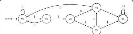
The two problems can be solved by first considering the language recognized by the seed π, in this context the at least one hit regular language, and its associated DFA. As an illustration, Fig. 1 displays the at least one hit DFA for the spaced seed 1101: this automaton recognizes the associated regular language {0,1}∗(1101|1111){0,1}∗, or less formally, any binary alignment sequence x that has at least one occurrence of 1101 or 1111 as a factor.
The second step consists in computing, by using a sim-ple dynamic programming (DP) procedure set for any states of the DFA and for each step i∈
1. . . ℓ ,
a. Either, the probability to reach any of the automaton states.
b. Otherwise, the minimal number of mismatch sym-bols 0 that have been crossed to reach any state.
For example, considering the probability problem (a) on a Bernoulli model where a match has a probability p set to 0.7, we show it can be computed—by first “replacing”, on the automaton of Fig. 1, the transition symbols 0 and 1 by their respective probabilities 0.3 and 0.7—then, on each step i, it is possible to compute the probability P(i,q) to reach each of the states q by applying a recursive formula
that uses the probability to be at any of its preceding states on step i−1. For the automaton of Fig. 1, this gives
i= 0 P(0, q1) = 1.0
other statesq have aP(0, q) = 0.0 i= 1 P(1, q1) = P(0, q1 orq2 orq4)×0.3
= P(0, q1) +P(0, q2) +P(0, q4) ×0.3 = (1.0 + 0.0 + 0.0)×0.3 = 0.3 P(1, q2) =P(0, q1)×0.7 = 1.0×0.7 = 0.7
other statesq have aP(1, q) = 0.0 i= 2 P(2, q1) = P(1, q1 orq2 orq4)×0.3
= P(1, q1) +P(1, q2) +P(1, q4) ×0.3
= (0.3 + 0.7 + 0.0)×0.3 = 0.3 P(2, q2) =P(1, q1)×0.7 = 0.3×0.7 = 0.21 P(2, q3) =P(1, q2)×0.7 = 0.7×0.7 = 0.49 other statesq have aP(2, q) = 0.0
i= 3 P(3, q1) = P(2, q1 orq2 orq4)×0.3 = P(2, q1) +P(2, q2) +P(2, q4) ×0.3 = (0.3 + 0.21 + 0.0)×0.3 = 0.153
P(3, q2) =P(2, q1)×0.7 = 0.3×0.7 = 0.21 P(3, q3) =P(2, q2)×0.7 = 0.21×0.7 = 0.147 P(3, q4) = P(2, q3 orq5)×0.3
= P(2, q3) +P(2, q5) ×0.3 = (0.49 + 0.0)×0.3 = 0.147 P(3, q5) =P(2, q3)×0.7 = 0.49×0.7 = 0.343 P(3, q6) = 0.0
i= 4 . . .
on step i=4, the probability to reach the final state q6 can be computed to P(4,q6)=0.343 ( 0.73 ), as a logical (and first non-null) probability for the seed π=1101 to detect alignments of length ℓ=4—on step i=5, the prob-ability to reach q6 can be computed to P(5,q6)=0.51793 (0.73×(1+0.3+0.7×0.3)) to detect alignments of length ℓ=5 .
Another example, considering now the lossless prop-erty (b) for the spaced seed π=1101: we can show that this seed is lossless for one single mismatch, when ℓ≥6 (but computational details are left to the reader, after a remark on tropical semi-rings in the next paragraph): the seed is thus (ℓ=6,k=1)-lossless ; however, this seed is not (ℓ=5,k=1)-lossless, since reading the consistent sequence 10111 leads to a non-final state.
Finally, we simply mention that this second computa-tional step involves the implicit use of semi-rings,
a. Either probability semi-rings: (E=R0≤r≤1, ⊕ = +,
⊗ = ×, 0⊕,ǫ
⊗ =0, 1⊗=1) ; the final state(s) of the
DFA give(s) the probability of having at least one hit after ℓ steps of the DP algorithm,
b. Otherwise tropical semi-rings: (E=R≥0, ⊕ =min, ⊗ = + 0⊕,ǫ
⊗ = ∞, 1⊗=0). The seed is (ℓ,k) -loss-less iff all the non-final states of the DFA have a mini-mal number of mismatches that is strictly greater than k, after ℓ steps of the DP algorithm.2
2 The opposite is equivalent to say that at least one string of length ℓ with ≤k mismatches is not hit by the seed; in other words, that the seed is not (ℓ,k) -lossless. Note that k does not need to be initially set: it can be estimated using this requirement, even after the DP run.
q1
start q2 q3
q4
q5
q6 0
1
0
1
0
1 0
1
0 1
0,1
Semi‑rings and number of alignments
Semi-rings are a flexible and powerful tool, employed for example to compute probabilities, scores, distances, counts (to name a few) in a generic dynamic program-ming framework [82, 83]. The first problem involved, mentioned at the end of the previous section, is the right choice of the semi-ring, adapted to the question being addressed. Sometimes, selecting an alternative semi-ring to count elements, may turn out to be a flexible choice that solves more involved problems (for example comput-ing probabilities is one of them, and will be described in next section).
Counting semi-rings [84] are adapted for this task: when applied on the right language and its right
automaton, they can report the number of alignments
cπ,m that are at the same time detected by the seed π while having m matches out of ℓ alignment symbols. The main idea that enables the computation of these
cπ,m counting coefficients (illustrated on Fig. 2 as the intersection product) is first to intersect the language recognized by the seed π (the at least one hit language of π) with the classes of alignments that have exactly m matches: the automaton associated with all of these classes of alignments with m matches has a very simple linear form with ℓ+1 states, where several distinct final states are defined according to all the possible values of m∈ [0. . . ℓ]. Finally, since the intersection of two regu-lar languages is reguregu-lar [Theorem 4.8 of the timeless 85],
×
start q1 q2q3
q4
q5
p0 start
p1
p2
p−1
p
p0×q1 start
p1×q1 p1×q2 p1×q4
p2×q1 p2×q2 p2×q3 p2×q4 p2×q5
p−1×q1 p−1×q2 p−1×q3 p−1×q4 p−1×q5
p ×q1 p ×q2 p ×q3 p ×q4 p ×q5
0
1
0 1
0
1 0
1 0,1
0
1
0
1
0
1
0
1
0,1
0
1
0
1
0
1 0
1
0
1
0
1
0
1 0
1
0
1
0
1
0
1
0
1 0
1
0
1
0 1
0
1 0
1 0
1 0,1
it can thus be represented by a conventional DFA, while keeping the feature of having several distinct final states.
As an illustration, Fig. 2 displays the at least one hit DFA for the spaced seed 101 (on the top), the lin-ear 1-counting DFA (on the vertical left part) to isolate alignments with exactly m matches, and finally their intersection product, that represent the intersecting language as a new DFA (itself obtained by crossing synchronously the two previous DFAs). Note that each of the final states pm×q5 (for m< ℓ) of the resulting DFA is reached by alignment sequences with exactly m matches that are also detected by the seed 101 (unless for the last state pl×q5, where ≥ℓ matches may have been detected).
Then, starting with the empty word (counted once from the initial state p0×q1), it is then possible to count the number of words of size one (two words 0 and 1 on a binary alphabet) by following transitions from the initial state to p0×q1 and p1×q2, respec-tively; from the (two) states already reached, it is then possible to count words of size two (four words on a binary alphabet), and so on, while keeping, for each DFA state pm×qj and on each step i, a single count record, which represents the size of the subset of the partition of the 2i words that reach pm×qj.
Note that, for a seed π of weight wπ and span sπ (thus with sπ−wπ don’t-care symbols), the at least one hit automaton size is in O(wπ2sπ−wπ), so the intersection with the classes of alignments that have m matches out of ℓ leads to a full size in O(ℓwπ2sπ−wπ): the
compu-tational complexity of the algorithm can thus be esti-mated in O(ℓ2wπ2sπ−wπ) in time and O(ℓwπ2sπ−wπ) in
space. As shown by [1], it can be processed incremen-tally for all the alignment lengths up to ℓ, with the only restriction that the numbers of alignments per state (≤2ℓ) fit inside an integer word (64 or 128bits).
We first mention that a breadth-first construction of the intersection product can be used to limit the depth of the reached states to ℓ. We have already noticed that several authors have performed equivalent tasks with a matrix for the full automaton [86], or with a vector for each automaton state [1], probably because contiguous memory performance is better. An advantage of such lazy automaton product evaluation may be that, besides the fact that it is a generic automaton product, we avoid sparse data-structures combined with many non-reachable states (for example, pℓ−1×q1 and pℓ×q1 will never be reached on any sequences of size ℓ >2: since two mismatches are needed to reach them, then pm must always have its associated number of matches m≤ℓ−2).
We finally mention that a similar method was used in [87] to compute correlation coefficients between the
seed number of hits or the seed coverage, and the true alignment Hamming distance.3
In the following sections, we will use the (m-matches counting) cπ,m coefficients to compute, either probabili-ties on continuous models, or frequencies on discrete models.
Continuous models
Bernoulli polynomial form and dominance between seeds Once the cπ,m coefficients (the number of alignments of length ℓ with m matches that are detected by the seed
π ) are determined, the probability to hit an alignment of length ℓ under a Bernoulli model (where the probability of having a match is p) can be directly computed as a poly-nomial over p of degree at most ℓ:
The expression (1) was first proposed by [1] for spaced seeds, noticing that each alignment with m match symbols and ℓ−m mismatch symbols, “no matter how arranged”, has the same probability pm(1−p)ℓ−m to occur. The coefficient cπ,m then gives the number of such (obviously independent) alignments that are detected by the seed π. This leads, for all the possible number of match/mismatch symbols in an alignment of length ℓ, to the expression (1)
of the sensitivity for π. At first sight, we would conclude that this formula might be numerically unstable without any adapted computation, due to large cπ,m coefficients, opposed to rather small pm(1−p)ℓ−m probability values. But we will see that this expression (1) is not so frequently evaluated, and when it is, requires more involved tools than a classical numerical computation.
Mark and Benson [1] also include in their paper an elegant and simple partial order named dominance between seeds: suppose that two spaced seeds πa and
πb have to be compared according to their respec-tive cπa,m and cπb,m coefficients: now, assume that,
∀m∈ [0. . . ℓ] cπa,m≥cπb,m (with at least a single dif-ference on at least one of the coefficients), then we can conclude that πadominatesπb, and thus that πb can be discarded from the possible set of optimal seeds. Indeed, the sensitivity, defined by the formula (1) as a sum of same positive terms pm(1−p)ℓ−m , each term being respectively multiplied by a seed-dependent positive coef-ficient cπ,m, guarantee that the sensitivity of πb will never be better than the sensitivity of πa, whatever parameter p∈ [0, 1] is chosen.
3 Technical details at
http://bioinfo.cristal.univ-lille.fr/yass/iedera_cover-age/index_additional.html.
(1)
Prπ(p,ℓ)=cπ,0p0(1−p)ℓ+cπ,1p1(1−p)ℓ−1+ · · ·
In practice, from the initial set of all the possible seeds of given weight w and maximal span s, several seeds can be discarded using this dominance principle, reducing the initial set to a small subset of candidate seeds to optimal-ity. But this dominance principle is a partial order between seeds: this signifies that some seeds cannot be compared.
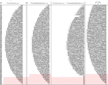
As an illustration, Table 1 lists the cπ,m coef-ficients of two single seeds, the contiguous seed (11111111111), and the Patternhunter I spaced seed (111010010100110111), for the alignment length ℓ=64. Note that comparing only the pairs of coefficients c11111111111,m and c111010010100110111,m does not help in choosing/discarding any of the two seeds by the dominance principle, since
c11111111111,m>c111010010100110111,m when m≤18 , or c11111111111,m≤c111010010100110111,m otherwise (with a strict inequality when m≤59). Actually, both seeds are included in the set of the dominant seeds of weight w=11 found on alignments of length ℓ=64, as mentioned by [1], and verified in our experiments.
Surprisingly, according to the experiments of [1], very few single seeds are overall dominant in the class of seeds of same weight w and fixed or restricted span s (e.g. s≤2×w) : this dominance criterion was thus used as a filter for the pre-selection of optimal seeds. In the section “Experiments” , we show that the domi-nance selection also scales reasonably well for select-ing multiple seeds candidates.
Hit Integration and its associated polynomial form
Hit Integration (HI) for a given seed π was proposed by [2] as
pb
pa Prπ(p,ℓ)dp
pb−pa for a given interval [pa,pb] (with 0≤pa<pb≤1), where Prπ(p,ℓ) is the probability for the seed π to hit an alignment of length ℓ generated by
a Bernoulli model of parameter p, as mentioned at the beginning of the previous part.
The main idea behind this integral formula is that, to cope with a “once set” and “single” p value that gives higher probabilities to alignments with percent
Table 1 Polynomial coefficients
m c11111111111,m vs c111010010100110111,m c11111111111,m−c111010010100110111,m =64m
11 54 > 47 +7 3284214703056
12 2809 > 2491 +318 13136858812224
13 71656 > 64766 +6890 47855699958816
14 1194726 > 1101022 +93704 159518999862720
15 14641250 > 13762775 +878475 488526937079580
16 140614565 > 134875195 +5739370 1379370175283520
17 1101959040 > 1079001425 +22957615 3601688791018080
18 7244724760 > 7244718291 +6469 8719878125622720
19 40770844660 < 41657015519 -886170859 19619725782651120
20 199422609750 < 208283509933 -8860900183 41107996877935680
21 857960383280 < 916431510317 -58471127037 80347448443237920
22 3277621380677 < 3582286065137 -304664684460 146721427591999680
23 11204891663658 < 12537156246105 -1332264582447 250649105469666120 24 34497110919250 < 39535559114049 -5038448194799 401038568751465792 25 96159187213600 < 112936248584277 -16777061370677 601557853127198688 26 243763479345750 < 293540495751220 -49777016405470 846636978475316672 27 564093286500926 < 696814345058019 -132721058557093 1118770292985239888 28 1195421472109319 < 1515471845391157 -320050373281838 1388818294740297792 29 2326215369539880 < 3027659295087000 -701443925547120 1620288010530347424 30 4166062298664175 < 5568629383085086 -1402567084420911 1777090076065542336 31 6879820141519780 < 9446128578860855 -2566308437341075 1832624140942590534 32 10492775658436071 < 14799578653936876 -4306802995500805 1777090076065542336 33 14798700315741024 < 21439532801385436 -6640832485644412 1620288010530347424 34 19320389713130985 < 28740508306965946 -9420118593834961 1388818294740297792 35 23366558713472100 < 35669405026997193 -12302846313525093 1118770292985239888 37 27219853884514060 < 43615425947917806 -16395572063403746 846636978475316672 38 26225237830956885 < 42947005673390702 -16721767842433817 601557853127198688 39 23419576997614252 < 39105472634332839 -15685895636718587 401038568751465792 40 19375279711450000 < 32890005171748738 -13514725460298738 250649105469666120 41 14838407971200840 < 25512761744419311 -10674353773218471 146721427591999680 42 10508138298881405 < 18217341897718037 -7709203598836632 80347448443237920 43 6871432453555670 < 11945918621774786 -5074486168219116 41107996877935680 44 4141671553771500 < 7173408931309221 -3031737377537721 19619725782651120 45 2295920726320600 < 3931419207110065 -1635498480789465 8719878125622720 46 1167451399456015 < 1958941918042764 -791490518586749 3601688791018080 47 542811202068762 < 883659819808009 -340848617739247 1379370175283520 48 229916824107023 < 359224789199125 -129307965092102 488526937079580 49 88333146992720 < 131012177925790 -42679030933070 159518999862720 50 30629979651075 < 42697694041897 -12067714390822 47855699958816 51 9532295505880 < 12400365695291 -2868070189411 13136858812224 52 2645918048566 < 3205551423838 -559633375272 3284214703056 53 650712755004 < 737766347839 -87053592835 743595781824 54 140817870050 < 151204825507 -10386955457 151473214816
55 26634941702 < 27534130189 -899188487 27540584512
56 4374599544 < 4426105322 -51505778 4426165368
57 619583272 < 621216072 -1632800 621216192
58 74955853 < 74974368 -18515 74974368
59 7624506 < 7624512 -6 7624512
60 635376 = 635376 0 635376
61 41664 = 41664 0 41664
62 2016 = 2016 0 2016
63 64 = 64 0 64
64 1 = 1 0 1
identities close to p, a given interval [pa,pb] is more suitable. In terms of the generative process,
pb
paPrπ(p,ℓ)dp
pb−pa can be interpreted as choosing uniformly a value for the Bernoulli parameter p in the range [pa,pb], each time and once per alignment sequence, before run-ning the Bernoulli model to generate this full alignment sequence x of length ℓ.
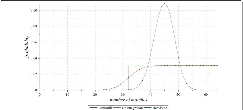
An illustration of the full probability mass function for the Hit Integration compared with the Bernoulli and the Heaviside distributions (the latter is defined in the next section) is given in Fig. 3 for alignments of length
ℓ=64.
Chung and Park [2] pointed out that designed spaced seeds were of different shapes, and that several seeds obtained on [pa=0,pb=1] or [pa=0.5,pb=1] were in practice better (compared with three other criteria tested in their paper). We also noticed that the method of [2] was modeled on the [27] recursive decomposi-tion, and is based on a very careful and non-trivial anal-ysis of the terms Ik[i,b] defined by :
with i: position along alignment, b: align-ment suffix that is also π-prefix hitting, over the parameter k∈|b|1. . . ℓ−i+ |b|
, and their rela-tionship: this leads to their recurrence formula
Ik[i,b] =
pk×Prπ
�i,b�dp
Ik[i,b] =Ik[i,b0] +Ik+1[i,b1] −Ik+1[i,b0] computed with the [27] algorithm scheme, using an additional internal loop layer for k ∈ [|b|1. . . ℓ−i+ |b|], and a non-obvious ordering of the computed terms on k vs |b| to remain DP-tractable.
Even if the algorithm we propose to compute the Hit Integration (in the next paragraph) has the same theoretical worst case complexity, its advantages are twofold:
• We propose a dynamic programming algorithm that is strictly equivalent to the one previously pro-posed for the the Bernoulli model : in fact, both model-dependent algorithms can even pool their most time-consuming part. Moreover, the automa-ton used by the dynamic programming algorithm can be previously minimized: this reduction is greatly appreciated when multiple seeds are pro-cessed.
• We propose a parameter-free approach for the pa
or pb parameters: it is therefore possible to
com-pute, on any interval, how far a seed is optimal; moreover, we will show that the dominance crite-rion can be applied as a pre-processing step.
The Hit Integration pb
pa Prπ(p,ℓ)dp can be rewritten by applying the polynomial formula (1) into:
Fig. 3 Bernoulli, Hit Integration, and Heaviside models. The Bernoulli (for p=0.7), the 1.0
0.5 Hit Integration, and the 1
1
2 Heaviside probability mass functions of the number of matches, on alignments of length ℓ=64. Highlighted dots indicate the weights given for each alignment class with a given number of matches m out of ℓ alignment symbols, under each of the three models. Note that, since the sum of the weights is always 1 for any model, and since the class of alignments with exactly m=32 matches out of ℓ=64 is fully included in 1
1
2 Heaviside model but only half-included in 1.0
Two interesting features can then be deduced from this trivial rewriting.
First, for any constant integers u and v, since the integral of the polynomial part
pb
pa p
u(1−p)vdp=pu+1v k=0
v
k (−p)k
u+k+1
pb
pa can be
easily computed (as a larger degree polynomial), the integral of the right part of the formula (2) can be pre-computed independently of the counting coefficients
cπ,m, and thus independently of the seed π. Thus, only cπ,m coefficients characterize the seed π for both the
Bernoulli model and the Hit Integration model.
Moreover, we can see that, for 0≤pa<pb≤1 and
for all m∈ [0. . . ℓ], the integral papbpm(1−p)ℓ−mdp of the right part of the formula (2) is always positive. Therefore, the dominance between seeds also can be directly applied on the cπ,m coefficients to select
domi-nant seeds before computing the Hit Integration (for any range [pa,pb]) by applying the formula (2), thereby
saving computation time for the optimal set of seeds. As a consequence, even if the optimal seeds selected from the Bernoulli and the Hit Integration models may
(2)
pb
pa
Prπ(p,ℓ)dp=
pb
pa
ℓ
m=0
cπ,mpm(1−p)ℓ−mdp
=
ℓ
m=0 cπ,m
pb
pa
pm(1−p)ℓ−mdp
have different shapes, all such optimal seeds are guar-anteed to be dominant4 in the sense of [1]. Note that the dominance of a seed can be computed indepen-dently of any parameter p, or here, any parameters [pa,pb]: the dominance criterion can thus be used to
pre-select seeds using exactly the same process pro-posed at the end of the previous part.
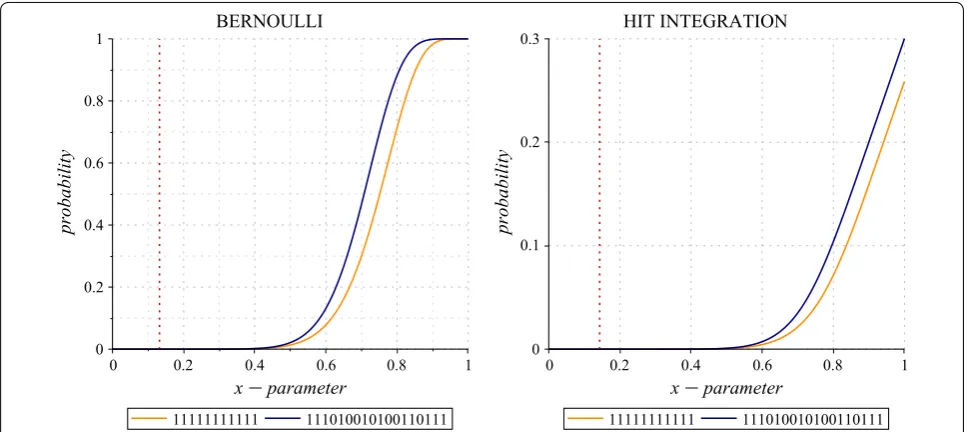
As an illustration, Fig. 4 plots the Bernoulli (left) and the x
0 Hit Integration (right) polynomials of two seeds: the contiguous seed (11111111111) and the Pattern-hunter I spaced seed (111010010100110111) which are the two already mentioned out of the forty domi-nant seeds of weight w=11 on alignments of length ℓ=64. Note that the Patternhunter I spaced seed, when compared to the contiguous seed, turns out to be better, if we consider the Bernoulli criterion only when
p>0.13209 (dark red dashed line)5, or if we consider the x
0 Hit Integration criterion only when x>0.14301 (dark red dashed line). However, if one wants to con-sider, not the x
0, but the 1
x Hit Integration criterion (data not shown), then the Patternhunter I spaced seed will always outperform the contiguous seed, even if both seeds are dominant in terms of cπ,m coefficients
and cannot be directly compared at first with this par-tial order dominance.
4 This side result is not discussed in [2], probably because they were more interested by the seed rank and not necessary the “optimal seed”, which they sometime called “dominant”.
5 As already observed by [63]. Fig. 4 Bernoulli and Hit Integration polynomials. The Bernoulli and x
0 Hit Integration polynomials plots for the contiguous seed and the Pattern-hunter I spaced seed, on alignments of length ℓ=64. The two polynomials have been plotted according to their respective formulas (1) and (2).
A vertical mark indicates where they cross each other in the range x∈ ]0, 1[ : the contiguous seed is better under this marked value; otherwise, the
We finally mention that, for alignments of length ℓ=64, both the contiguous seed and the Pattern-hunter I seed are in the set of the twelve optimal seeds found for the Bernoulli model6 (they are reported by symbols 0 and R in Fig. 5, top line of the first plot). Both are also in the set of the eight optimal seeds for the x
0 Hit Integration model. But, quite surprisingly, neither of the two is in the set of the four optimal seeds for the 1
x Hit Integration model (reported in Fig. 6, top
line of first plot). In fact, for the 1
x Hit Integration
model, the spaced seed 111001011001010111
(reported by a symbol O in Fig. 6, top line of first plot) is optimal7 on a wide range of x (x∈ [0, 0.97189]) before being surpassed by three other seeds (K , P and N in Fig. 6, top line of the first plot).
Discrete models and lossless seeds
In this section, we propose two additional models for selecting seeds. We will name them Dirac and Heaviside. These models can be seen as the discrete counterparts of the Bernoulli and the Hit Integration models, and are simply defined by:
1 Diracπ(m,ℓ)= cm,π (ℓ
m), to give the ratio between the
number of alignments detected by the seed π over all
the alignments of length ℓ with exactly m matches,
2 Heavisideπ(ma,mb,ℓ)= mb
m=maDiracπ(m ,ℓ)
mb−ma+1 , to give the average ratio, over any number of matches m between ma and mb (out of ℓ) of the previously
defined Dirac model. The Heaviside full distribution has already been illustrated in Fig. 3, together with the Hit Integration distribution with similar param-eters.
As long as we allow the possible loss of some of the strictly equivalent8 seeds in terms of sensitivity defined
6 As already mentioned by [1].
7 As already mentioned by [2], but for the non-parametrized 1 0 and
1
1 2 Hit Integration model.
8 To give a quick and intuitive example, we consider an extreme case : an alignment of fixed length ℓ without any mismatch symbol. Any seed π of
weight wπ≤ℓ and span sπ≤ℓ obviously detects this alignment, whatever
its shape is, so Diracπ(m=ℓ,ℓ) and Heavisideπ(ma=ℓ,mb=ℓ,ℓ) reach
their maximal sensitivity of 1. For a given weight w, the restriction of all these seeds to dominant seeds implies that many are lost when dominance selection is applied to keep the best representatives.
by the Dirac and Heaviside functions, the dominance criterion can be applied to filter out many candidate seeds.
In addition, the Dirac and Heaviside functions are based on rational number computations/comparisons: they are thus one or two orders of magnitude faster and lighter to compute and store, compared to the polyno-mial forms given by the continuous models of the previ-ous section.
Finally, an interesting feature of the Diracπ(m,ℓ), also true for the specific Heavisideπ(m,ℓ,ℓ), is that, when the number of match symbols m is large enough, one seed π (or sometime several seeds) can meet the equality
cπ,m′ =ℓ
m′
for all m′≥m. Such seeds are thus lossless since they can detect all the alignments of length ℓ with at least m matches (or with at most ℓ−m mismatches), and obviously the best lossless ones are retained in the set of dominant seeds, when the equality cπ,m=
ℓ
m
occurs. As a side consequence, the best lossless seeds are also in the set of dominant seeds and will be reported in the experiments.
Note that, to keep a symmetric notation with the pb
pa
Hit Integration, and also have the same range for the domain of definition (0≤pa<pb≤1), we will use
the “frequency” notation fb
faHeaviside to designate
Heaviside(⌊ℓ×fa⌋,⌊ℓ×fb⌋,ℓ). We will also rescale the Dirac function on the Bernoulli’s domain of defini-tion, by using the frequency f (0≤f ≤1) to designate Dirac(⌊ℓ×f⌋,ℓ).
Experiments
Single spaced seeds (n=1) and multiple co-designed spaced seeds (n∈ [2. . .4]) of weight w∈ [3. . .16] and span s at most 2×w have been considered. Note that, for single seeds of large weight (w≥15), or for multiple seed, the full enumeration is respectively burdensome or intractable, so we prefer to apply the hill-climbing algo-rithm of Iedera [88]: selected dominant spaced seeds are thus locally dominant, since it would be computation-ally unfeasible to guarantee their overall dominance. All the spaced seeds are evaluated on alignments of length ℓ∈ [2×w. . .64].
The main idea during the evaluation, also used by [1] but only for the single Bernoulli criterion and on a single spaced seed, is to split the computation in two distinct stages:
(See figure on previous page.)
Fig. 5 Bernoulli and Dirac optimal seeds. The Bernoulli and Dirac optimal seeds, for single seeds of weight 11 and span ≤22, over the match probability or the match frequency of each model (x-axis), and on any alignment length ℓ∈ [22. . .64] (y-axis). On both Figs. 5 and 6, we choose
1 Selecting the set of dominant seeds is the first stage: it provides a reduced set of candidate seeds. Note that the dominant selection can be applicable with-out prior knowledge of the sensitivity criterion being used, provided that this sensitivity criterion is estab-lished on i.i.d sequence alignments (this last require-ment is true for the Bernoulli, the Hit Integration, the Dirac, and the Heaviside models).
2 Comparing each of the seeds from the set of domi-nant seeds with a sensitivity criterion is the second stage: it usually depends on at least one parameter (for example, for the Bernoulli model: the probabil-ity p to generate a match) which has different conse-quences on continuous and discrete models:
• For the Bernoulli and the Hit Integration continu-ous models, this implies comparing p-parametrized or [pa,pb]-parametrized polynomials: we follow the idea proposed in [1] for the Bernoulli model and also apply it on the Hit Integration model where we compute the x
0 HI and the
1
x HI respectively. Let us concentrate on the Bernoulli model with a (single) free parameter p: For two dominant seeds πa and πb
and a given length ℓ, we compute their respective
polynomials Prπa(p,ℓ) and Prπb(p,ℓ) and their
dif-ference Prπa−πb(p,ℓ)=Prπa(p,ℓ)−Prπb(p,ℓ) (an example of its associated coefficients is illustrated on the third column of Table 1), from which zeros in the range p∈ [0, 1] are numerically extracted using solvers from maple or maxima. Using the p-intervals between these zeros, it is then possible to determine whether Prπa−πb(p,ℓ) is positive or negative, and thus which of the two seeds πa or πb
is better according to p. Finally, the Pareto envelope (optimal seeds) can be extracted from the initial set of dominant seeds.
• For the Dirac and the Heaviside discrete mod-els, this implies comparing, instead of real-valued polynomials, integer numbers for the Dirac model (and respectively rational numbers for the Heavi-side model), which is an easier and lighter process. The Pareto envelope can then be easily extracted from these discrete models to select the optimal seeds from the set of dominant seeds. We have also
extracted the lossless part for the Dirac and the 1
x Heaviside criteria.
In the aforementioned experiments, we noticed that the size of the set of dominant seeds was at most 3359 (with a median size of 57 and an average size of 303 for all the experiments). To briefly illustrate this point, a list of each maximum size in our experiments is provided on Table 2.
So far, we restricted the span of our designed seeds to 2×w, and also did not consider one single fixed proba-bility p during the optimization process. These restrictive conditions could be of course alleviated, but we mention here that computed sensitivities are close to (even if not strictly speaking “better than”) the top ones mentioned in several publications [56, 77, 78, 80] where the emphasis was on the heuristic being used for designing seed, the speed of the optimization algorithm, and the best seed for a fixed probability p. Table 3 has been extracted from the Table 1 of recently published paper [80] and summa-rizes known optimal sensitivities.
Note that we did not use any Overlap
Complexity/Covariance heuristic optimisation here (to stay in a generic framework), and simply apply the very simple hill-climbing algorithm of Iedera. We also men-tion that our seeds are not definitely the best ones, but since they are published, their sensitivity can be checked using other software, as mandala [63], SpEED [56], or ras-bhari [80] ([43, 57] did the same with the seeds obtained with the SpEED software).
Finally, to show a typical output of this generalized parameter-free approach, optimal single (n=1) seeds of weight w=11 have been plotted according to the main parameter of each model (horizontal axis) and the length ℓ of the alignment (vertical axis) in Figs. 5 and 6. On dis-crete models, a pink mark represents the lossless border: seeds on the right of this border are by essence lossless for the set of parameters. On the right margin of the discrete models, we indicate the fraction of the minimum number of matches m over the alignment length ℓ to be lossless.
We provide the scripts and the whole set of single and multiple seeds, in http://bioinfo.cristal.univ-lille.fr/yass/ iedera_dominance in the hope this will be useful to align-ment software and spaced seeds alignalign-ment-free metagen-omic classifiers.
(See figure on previous page.)
Fig. 6 Hit Integration and Heaviside optimal seeds. The 1
x Hit Integration and 1x Heaviside optimal seeds, for single seeds of weight 11 and span
≤22, over the match probability or the match frequency of each model (x-axis), and on any alignment length ℓ∈ [22. . .64] (y-axis). On both Figs. 5
and 6, we choose to represent the same seeds with the same label and with the same background color. On discrete models, a pink mark is set. Seeds on the right of this mark are lossless for the two parameters indicated on the right margin: the minimum number of matches m over the alignment length
Discussion
In this paper, we have presented a generalization of the usage of dominant seeds, first on the Hit integration model with a parameter-free approach, and also on two new discrete models (named Dirac and Heaviside) that are related to lossless seeds. In this parameter-free con-text, we show that all these models can be computed with help of a method for counting alignments of particular classes, themselves represented by regular languages, and a counting semi-ring to perform an efficient set size computation.
We open the discussion with the complementary asymptotic problem, before going to finite but multivari-ate model extensions.
Complementary asymptotic problem
So far, we only have considered a set of finite alignment lengths ℓ to design seeds. But limiting the length is far from satisfactory, so the next problem deserves consid-eration too: the asymptotic hit probability of seeds [63, 89–91].
As an example, if we consider the Bernoulli model where we choose p in the interval ]0, 1[, and then con-sider the probability Prπ(p,ℓ) for π to hit an alignment of length ℓ (noted Prπ(ℓ) to simplify), then it can be shown that the complementary probability Prπ(ℓ) [see for exam-ple 91, equation (3)] follows
Here π is the largest (positive) eigenvalue of the sub-sto-chastic matrix of π where final states have been removed, this matrix computing thus the distribution Prπ(ℓ) when powered to ℓ (see section 3.1 π and βπ of [63]).
As an example, for p=0.7 and for the Patternhunter I spaced seed, we have (with help of a Maple script) {,β}111010010100110111= {0.98731, 0.22667}, that can
lim
ℓ→∞Prπ(ℓ)=βπ
ℓ π
1+o(1)
be compared with the contiguous seed of same weight {,β}11111111111= {0.99364, 0.44784}. [63] have proven that, in the class of seeds with the same weight, contigu-ous seeds have the largest value and thus are the asymp-totic worst-case in terms of hit probability, a trait shared with the uniformly spaced seeds of same weight (e.g. 101010101010101010101 or 1001001001001001 001001001001001).
Comparing seeds asymptotically can thus be done eas-ily by comparing their respective eigenvalue, or their β when equality occurs, but it seems to be
computation-ally possible9 only if p is set numerically before the analysis.
Moreover dominant seeds’ extracted from this paper on a limited alignment length ℓ (here ℓ≤64) would not always be optimal for any ℓ: such seeds can, however, be justified as “good” candidates for seeds of restricted span (e.g. s≤2×w), but definitely not the optimal ones, unless dominance is computed on a wider range of align-ment length ℓ values.
For example, the best (smallest) for any
domi-nant seed of weight w=11 and span at most 2×w , on alignments of length ℓ≤64 is 0.98714 for the seed 1110010100110010111. Surprisingly, even if this seed reaches the smallest out of its dominant class, it never occurred in the optimal seeds, in any of our experi-ments. Moreover, we have checked that another seed 1110010100100100010111 has an even smaller =0.98669: this last seed was not dominant for ℓ≤64, but would be in the class of seeds of span at most 2×w if larger values of ℓ were selected.
Finally, a parameter-free analysis implying both p and ℓ seems difficult to apply for large seeds. It is interesting to notice that several of our preliminary experiments
9 At least to the author, but this parametrized problem is intrinsically inter-esting in itself.
Table 2 Maximum size of the set of dominant seeds
For n seeds of weight w, we indicate the maximum size of the dominant set found in our experiments on all the alignment lengths ℓ∈ [s. . .64]. We also give the largest alignment length (ℓ) where this maximum has been reached
w
n 3 4 5 6 7 8 9 10 11 12 13 14 15 16
1 2 7 8 13 15 26 23 32 40 45 46 48 74 84
(64) (64) (62) (64) (64) (61) (60) (62) (64) (63) (64) (59) (64) (64)
2 5 12 35 41 52 99 128 197 231 207 350 320 439 376
(64) (63) (63) (61) (64) (64) (60) (62) (61) (59) (63) (64) (64) (41)
3 6 26 85 84 204 320 391 485 854 932 1103 1449 1508 1812
(60) (64) (64) (62) (64) (60) (56) (56) (62) (64) (64) (41) (64) (63)
4 7 29 124 190 254 535 811 1041 1450 1908 1775 2364 3125 3359
suggest that, asymptotically, and only10 for a restricted set of seeds (e.g. of weight w=11 and span at most 2×w), one seed is optimal whatever the value of p. This remains to be confirmed experimentally and theoretically because it might be possible that special cases exist, where at least two (or even more) seeds share the p partition.
Models and multivariate analysis
As far as i.i.d sequences are considered, the full frame-work of [1], including the dominant seed selection, can be applied on any extended spaced seed model (such as transition constrained seeds, vector seeds, indel seeds,...). However, additional free-parameters (such as the transi-tion/transversion rate, the indel/mismatch rate, ...) lead to an increase in the number of alignment classes (for exam-ple, alignments of length ℓ, with i indels, v transversion errors, t transitions errors, and remaining m matches, such that ℓ=i+v+t+m) that have to be considered by the dominance selection. Moreover, it involves a much more complex multivariate polynomial analysis, if more than one parameter is, at this point, left free.
In a more general way, if i.i.d sequences are ignored, and dominant seed selection thus abandoned in its original form, one could mix several numerically-fixed models: for example, mixing a given HMM representing coding sequences, with a numerically-fixed Bernoulli model. The idea is here to use a free probability parameter to create a balance between the two models: either initially before generating the alignment, to choose each of the two mod-els; or along the alignment generation process, to switch
10 This restricted set of seeds condition is necessary: if removed, best seeds span will increase along ℓ, see [18].
between each of the two models. Seeds designed could thus be two-handed for analyzing both coding and non-coding genomic sequences at the same time, but with an additional control parameter that helps to change the known percentage of such genomic sequences. To com-pute the sensitivity in this model, a simple idea is to apply a polynomial semi-ring (with at least one parameter-free variable: here the one used to create the balance) on the automaton, and perform, not a numeric, but a symbolic computation.
Finally, as a logical consequence of the two previous remarks, we mention that any HMM with one (or pos-sibly several) free probability parameter(s) could always be analysed with a (multivariate) polynomial semi-ring, increasing thus the scope of the method to applications that depend on Finite State Machines : such parameter-free pre-processing can, at some point, be applied; more-over if several equivalence classes are established in term of probability, it may be possible to use equivalent domi-nance method to filter out candidates when comparing several elements.
Acknowledgments and funding
Donald E. K. Martin provided substantive comments on an earlier version of this manuscript. The author would like to thank the second reviewer for his/ her thorough review which significantly contributed to improving the quality of the paper. The publication costs were covered by the French Institute for Research in Computer Science and Automation (inria).
Competing interests
The author declare that he has no competing interests.
Availability of data and materials
All data and source code are freely available and may be downloaded from:
http://bioinfo.cristal.univ-lille.fr/yass/iedera_dominance/ Table 3 Sensitivity comparison of different programs
Italic values indicate the best sensitivity
The reported sensitivity for n=4 seeds of weight w on alignments of length l=50 under a Bernoulli model with a match probability p. All the reported results are extracted from the Table 1 of [80], but the last column that corresponds to our current public seeds, with a δ difference to the optimal seed
w p SpEED AcoSeed FastHC MuteHC Rasbhari Current sensitiv-ity (δ)
10 0.75 90.9098 90.9513 90.7312 92.6812 90.9614 90.8753 (1.8059%)
0.80 97.8337 97.8521 97.7625 98.3836 97.8554 97.8203 (0.5633%)
0.85 99.7569 99.7614 99.7431 99.8356 99.7618 99.7568 (0.0788%)
11 0.75 83.3793 83.4728 83.3068 83.4127 83.4679 83.4297 (0.0431%)
0.80 94.9861 95.037 94.9453 95.0194 95.0386 95.0127 (0.0259%)
0.85 99.2431 99.2478 99.2250 99.2486 99.2506 99.2452 (0.0054%)
12 0.80 90.5750 90.6328 90.4735 90.5820 90.6648 90.5571 (0.1077%)
0.85 98.1589 98.1766 98.1199 98.1670 98.1824 98.1591 (0.0233%)
0.90 99.8821 99.8853 99.8771 99.8836 99.8864 99.8840 (0.0024%)
16 0.85 84.8212 84.9829 84.6558 84.8764 84.969 84.9668 (0.0161%)
0.90 97.4321 97.4712 97.3556 97.4460 97.5035 97.4730 (0.0305%)
Consent for publication
Not applicable. The manuscript does not contain any data from any individual person.
Ethical approval
The manuscript does not report new studies involving any animal or human data or tissue.
Received: 19 September 2016 Accepted: 30 January 2017
References
1. Mak DYF, Benson G. All hits all the time: parameter free calculation of seed sensitivity. Bioinformatics. 2009;25(3):302–8.
2. Chung WH, Park SB. Hit integration for identifying optimal spaced seeds. BMC Bioinform. 2010;11(1):S37.
3. Ma B, Tromp J, Li M. PatternHunter: faster and more sensitive homology search. Bioinformatics. 2002;18(3):440–5.
4. Burkhardt S, Kärkkäinen J. Better filtering with gapped q-grams. Fund Inform. 2002;56(1—-2):51–70.
5. Brejová B, Brown DG, Vinař T. Vector seeds: an extension to spaced seeds. J Comput Syst Sci. 2005;70(3):364–80.
6. Burkhardt S, Kärkkäinen J. One-gapped q-gram filters for Levenshtein distance. Proceedings of the 13th symposium on combinatorial pattern matching (CPM), vol 2373, Lecture Notes in Computer Science Fukuoka (Japan). Berlin: Springer; 2002. p. 225–34.
7. Mak DYF, Gelfand Y, Benson G. Indel seeds for homology search. Bioinfor-matics. 2006;22(14):341–9.
8. Chen K, Zhu Q, Yang F, Tang D. An efficient way of finding good indel seeds for local homology search. Chin Sci Bull. 2009;54(20):3837–42. 9. Csűrös M, Ma B. Rapid homology search with neighbor seeds.
Algorith-mica. 2007;48(2):187–202.
10. Ilie L, Ilie S. Fast computation of neighbor seeds. Bioinformatics. 2009;25(6):822–3.
11. Chen W, Sung WK. On half gapped seed. Genome Inform. 2003;14:176–85.
12. Noé L, Kucherov G. Improved hit criteria for DNA local alignment. BMC Bioinform. 2004;5:149.
13. Yang J, Zhang L. Run probabilities of seed-like patterns and identifying good transition seeds. J Comput Biol. 2008;5(10):1295–313.
14. Zhou L, Stanton J, Florea L. Universal seeds for cDNA-to-genome com-parison. BMC Bioinform. 2008;9:36.
15. Frith MC, Noé L. Improved search heuristics find 20 000 new alignments between human and mouse genomes. Nucleic Acids Res. 2014;42(7):59. 16. Li M, Ma B, Kisman D, Tromp J. PatternHunter II: highly sensitive and fast
homology search. J Bioinform Comput Biol. 2004;2(3):417–39.
17. Sun Y, Buhler J. Designing multiple simultaneous seeds for DNA similarity search. J Comput Biol. 2005;12(6):847–61.
18. Kucherov G, Noé L, Roytberg MA. Multiseed lossless filtration. IEEE/ACM Trans Comput Biol Bioinform. 2005;2(1):51–61.
19. Farach-Colton M, Landau GM, Cenk Sahinalp S, Tsur D. Optimal spaced seeds for faster approximate string matching. J Comput Syst Sci. 2007;73(7):1035–44.
20. Kiełbasa SM, Wan R, Sato K, Horton P, Frith MC. Adaptive seeds tame genomic sequence comparison. Genome Res. 2011;21(3):487–93. 21. Peterlongo P, Pisanti N, Boyer F, Sagot MF. Lossless filter for finding long
multiple approximate repetitions using a new data structure, the bi-factor array. In: Consens M, Navarro G, editor. Proceedings of the 12th international conference, on string processing and information retrieval (SPIRE). Lecture Notes in Computer Science, vol 3772. Buenos Aires; 2005. p. 179–190. 22. Crochemore M, Tischler G. The gapped suffix array: a new index structure
for fast approximate matching. In: Chavez E, Lonardi S, editors. Proceed-ings of the 17th international—symposium on string processing and information retrieval (SPIRE), vol. 6393., Lecture notes in computer scien-ceLos Cabos: Springer; 2010. p. 359–64.
23. Onodera T, Shibuya T. An index structure for spaced seed search. In: Asano T, Nakano S-I, Okamoto Y, Watanabe O, editors. Proceedings of the 22nd international symposium on algorithms and computation (ISAAC),
vol. 7074., Lecture notes in computer scienceYokohama (Japan): Springer; 2011. p. 764–72.
24. Gagie T, Manzini G, Valenzuela D. Compressed spaced suffix arrays. In: Pro-ceedings of the 2nd international conference on algorithms for big data (ICABD). CEUR-WS, vol 1146. Palermo; 2014. p. 37–45.
25. Shrestha AMS, Frith MC, Horton P. A bioinformatician’s guide to the forefront of suffix array construction algorithms. Brief Bioinform. 2014;15(2):138–54.
26. Birol I, Chu J, Mohamadi H, Jackman SD, Raghavan K, Vandervalk BP, Ray-mond A, Warren RL. Spaced seed data structures for de novo assembly. Int J Genom. 2015;2015:196591.
27. Keich U, Li M, Ma B, Tromp J. On spaced seeds for similarity search. Discret Appl Math. 2004;138(3):253–63.
28. Nicolas F, Rivals É. Hardness of optimal spaced seed design. J Comput Syst Sci. 2008;74(5):831–49.
29. Ma B, Yao H. Seed optimization for i.i.d. similarities is no easier than opti-mal Golomb ruler design. Inf Process Lett. 2009;109(19):1120–4. 30. Schwartz S, Kent WJ, Smit A, Zhang Z, Baertsch R, Hardison RC, Haussler
D, Miller W. Human-mouse alignments with BLASTZ. Genome Res. 2003;13:103–7.
31. Darling AE, Treangen TJ, Zhang L, Kuiken C, Messeguer X, Perna NT. Procrastination leads to efficient filtration for local multiple alignment. Proceedings of the 6th international workshop on algorithms in bioinfor-matics (WABI), vol 4175. Lecture notes in bioinforbioinfor-matics. Zürich: Springer; 2006. p. 126–37.
32. Harris RS. Improved pairwise alignment of genomic dna. Ph.d. thesis, The Pennsylvania State University; 2007
33. Lin H, Zhang Z, Zhang MQ, Ma B, Li M. ZOOM! Zillions Of Oligos Mapped. Bioinformatics. 2008;24(21):2431–7.
34. Rumble SM, Lacroute P, Dalca AV, Fiume M, Sidow A, Brudno M. SHRiMP: accurate mapping of short color-space reads. PLoS Comp Biol. 2009;5(5):1000386.
35. Chen Y, Souaiaia T, Chen T. PerM: efficient mapping of short sequenc-ing reads with periodic full sensitive spaced seeds. Bioinformatics. 2009;25(19):2514–21.
36. Giladi E, Healy J, Myers G, Hart C, Kapranov P, Lipson D, Roels S, Thayer E, Letovsky S. Error tolerant indexing and alignment of short reads with covering template families. J Comput Biol. 2010;17(10):1397–411. 37. David M, Dzamba M, Lister D, Ilie L, Brudno M. SHRiMP2: Sensitive yet
practical short read mapping. Bioinformatics. 2011;27(7):1011–2. 38. Sović I, Šikić M, Wilm A, Fenlon SN, Chen S, Nagarajan N. Fast and sensitive
mapping of nanopore sequencing reads with GraphMap. Nat Commun. 2016;7:11307.
39. Preparata FP, Oliver JS. DNA sequencing by hybridization using semi-degenerate bases. J Comput Biol. 2005;11(4):753–65.
40. Tsur D. Optimal probing patterns for sequencing by hybridization. Pro-ceedings of the 6th international workshop on algorithms in bioinfor-matics (WABI), vol 4175. Lecture notes in bioinforbioinfor-matics. Zürich: Springer; 2006. p. 366–75.
41. Feng S, Tillier ERM. A fast and flexible approach to oligonucleo-tide probe design for genomes and gene families. Bioinformatics. 2007;23(10):1195–202.
42. Chung W-H, Park S-B. An empirical study of choosing efficient discrimi-native seeds for oligonucleotide design. BMC Genom. 2009;10(Suppl 3):3.
43. Ilie L, Ilie S, Khoshraftar S, Mansouri Bigvand A. Seeds for effective oligo-nucleotide design. BMC Genom. 2011;12:280.
44. Ilie L, Mohamadi H, Brian Golding G, Smyth WF. BOND: Basic Oligo Nucleotide Design. BMC Bioinform. 2013;14:69.
45. Kisman D, Li M, Ma B, Li W. tPatternhunter: gapped, fast and sensitive translated homology search. Bioinformatics. 2005;21(4):542–4. 46. Brown DG. Optimizing multiple seeds for protein homology search.
IEEE/ACM Trans Comput Biol Bioinform. 2005;2(1):23–38. 47. Roytberg MA, Gambin A, Noé L, Lasota S, Furletova E, Szczurek E,
Kucherov G. On subset seeds for protein alignment. IEEE/ACM Trans Comput Biol Bioinform. 2009;6(3):483–94.
48. Nguyen V-H, Lavenier D. PLAST: parallel local alignment search tool for database comparison. BMC Bioinform. 2009;10:329.
• We accept pre-submission inquiries
• Our selector tool helps you to find the most relevant journal
• We provide round the clock customer support
• Convenient online submission
• Thorough peer review
• Inclusion in PubMed and all major indexing services
• Maximum visibility for your research
Submit your manuscript at www.biomedcentral.com/submit
Submit your next manuscript to BioMed Central
and we will help you at every step:
50. Li W, Ma B, Zhang K. Optimizing spaced k-mer neighbors for efficient filtration in protein similarity search. IEEE/ACM Trans Comput Biol Bioinform. 2014;11(2):398–406.
51. Buchfink B, Xie C, Huson DH. Fast and sensitive protein alignment using DIAMOND. Nat Methods. 2014;12:59–60.
52. Somervuo P, Holm L. SANSparallel: interactive homology search against Uniprot. Nucleic Acids Res. 2015;43(W1):24–9.
53. Petrov I, Brillet S, Drezen E, Quiniou S, Antin L, Durand P, Lavenier D. KLAST: fast and sensitive software to compare large genomic data-banks on cloud. In: Proceedings world congress in computer science, computer engineering, and applied computing (WORLDCOMP). Las Vegas; 2015. p. 85–90.
54. Yang IH, Wang SH, Chen YH, Huang PH, Ye L, Huang X, Chao KM. Efficient methods for generating optimal single and multiple spaced seeds. In: Proceedings of the IEEE 4th symposium on bioinformatics and bioengineering (BIBE). Taichung: IEEE Computer Society Press; 2004. p. 411–16.
55. Ilie L, Ilie S. Multiple spaced seeds for homology search. Bioinformatics. 2007;23(22):2969–77.
56. Ilie L, Ilie S. SpEED: fast computation of sensitive spaced seeds. Bioin-formatics. 2011;27(17):2433–4.
57. Ilie S. Efficient computation of spaced seeds. BMC Res Notes. 2012;5:123.
58. Egidi L, Manzini G. Better spaced seeds using quadratic residues. J Comput Syst Sci. 2013;79(7):1144–55.
59. Egidi L, Manzini G. Design and analysis of periodic multiple seeds. Theor Comput Sci. 2014;522:62–76.
60. Egidi L, Manzini G. Spaced seeds design using perfect rulers. Fund Inform. 2014;131(2):187–203.
61. Egidi L, Manzini G. Multiple seeds sensitivity using a single seed with threshold. J Bioinform Comput Biol. 2015;13(4):1550011.
62. Brejová B, Brown DG, Vinař T. Optimal spaced seeds for homologous coding regions. J Bioinform Comput Biol. 2004;1(4):595–610. 63. Buhler J, Keich U, Sun Y. Designing seeds for similarity search in
genomic DNA. J Comput Syst Sci. 2005;70(3):342–63.
64. Preparata FP, Zhang L, Choi KP. Quick, practical selection of effective seeds for homology search. J Comput Biol. 2005;12(9):1137–52. 65. Kucherov G, Noé L, Roytberg MA. A unifying framework for seed
sensitivity and its application to subset seeds. J Bioinform Comput Biol. 2006;4(2):553–69.
66. Zhang L. Superiority of spaced seeds for homology search. IEEE/ACM Trans Comput Biol Bioinform. 2007;4(3):496–505.
67. Kong Y. Generalized correlation functions and their applications in selection of optimal multiple spaced seeds for homology search. J Comput Biol. 2007;14(2):238–54.
68. Noé L, Gîrdea M, Kucherov G. Designing efficient spaced seeds for SOLiD read mapping. Adv Bioinform. 2010;2010:708501.
69. Marschall T, Herms I, Kaltenbach H-M, Rahmann S. Probabilistic arith-metic automata and their applications. IEEE/ACM Trans Comput Biol Bioinform. 2012;9(6):1737–50.
70. Martin DEK, Noé L. Faster exact distributions of pattern statis-tics through sequential elimination of states. Ann Inst Stat Math. 2017;69:1–18.
71. Horwege S, Lindner S, Boden M, Hatje K, Kollmar M, Leimeister C-A, Morgenstern B. Spaced words and kmacs: fast alignment-free sequence comparison based on inexact word matches. Nucleic Acids Res. 2014;42(W1):7–11.
72. Leimeister CA, Boden M, Horwege S, Lindner S, et al., Morgenstern B. Fast alignment-free sequence comparison using spaced-word frequencies. Bioinformatics. 2014;30(14):1991–9.
73. Ghandi M, Mohammad-Noori M, Beer MA. Robust k-mer frequency estimation using gapped k-mers. J Math Biol. 2014;69(2):469–500. 74. Morgenstern B, Zhu B, Horwege S, Leimeister CA. Estimating
evolution-ary distances between genomic sequences from spaced-word matches. Algorithms Mol Biol. 2015;10:5.
75. Břinda K, Sykulski M, Kucherov G. Spaced seeds improve k-mer based metagenomic classification. Bioinformatics. 2015;31(22):3584–92.
76. Ounit R, Lonardi S. Higher classification sensitivity of short metagenomic reads with CLARK-S. Bioinformatics. 2016.
77. Duc DD, Dinh HQ, Dang TH, Laukens K, Hoang XH. AcoSeeD: an ant colony optimization for finding optimal spaced seeds in biological sequence search. Proceedings of the 8th international conference on swarm intelligence (ANTS), vol 7461. Lecture notes in computer science. Brussels: Springer; 2012. p. 204–11.
78. Do PT, Tran-Thi CG. An improvement of the overlap complexity in the spaced seed searching problem between genomic DNAs. In: Proceedings of the 2nd National Foundation for Science and Technology Develop-ment Conference on Information and Computer Science (NICS). Ho Chi Minh City; 2015. p. 271–76.
79. Gheraibia Y, Moussaoui A, Djenouri Y, Kabir S, Yin P-Y, Mazouzi S. Penguin search optimisation algorithm for finding optimal spaced seeds. Int J Softw Sci Comput Intell. 2015;7(2):85–99.
80. Hahn L, Leimeister C-A, Ounit R, Lonardi S, Morgenstern B. rasb-hari: optimizing spaced seeds for database searching, read map-ping and alignment-free sequence comparison. PLoS Comput Biol. 2016;12(10):1005107.
81. Choi KP, Zeng F, Zhang L. Good spaced seeds for homology search. Bioin-formatics. 2004;20(7):1053–9.
82. Allauzen C, Riley M, Schalkwyk J, Skut W, Mohri M. OpenFst: a general and efficient weighted finite-state transducer library. In: Holub J, Zdarek J, editors. Proceedings of the 12th international conference on implemen-tation and application of automata (CIAA), vol. 4783., Lecture notes in computer sciencePrague: Springer; 2007. p. 11–23.
83. Mohri M. Weighted automata algorithms. In: Handbook of weighted automata. Berlin: Springer; 2009. p. 213–54.
84. Huang L. Dynamic programming algorithms in semiring and hypergraph frameworks. Technical report, University of Pennsylvania, Philadelphia, USA; 2006.
85. Hopcroft JE, Motwani R, Ullman JD. Introduction to automata theory languages and computation. 3rd ed. New York: Pearson; 2007. 86. Aston JAD, Martin DEK. Distributions associated with general runs and
patterns in hidden Markov models. Ann Appl Stat. 2007;1(2):585–611. 87. Noé L, Martin DEK. A coverage criterion for spaced seeds and its
applica-tions to support vector machine string kernels and k-mer distances. J Comput Biol. 2014;21(12):947–63.
88. Kucherov G, Noé L, Roytberg MA. Iedera subset seed design tool. http:// bioinfo.lifl.fr/yass/iedera.php; 2016.
89. Ma B, Li M. On the complexity of spaced seeds. J Comput Syst Sci. 2007;73(7):1024–34.
90. Li M, Ma B, Zhang L. Superiority and complexity of the spaced seeds. In: Proceedings of the 17th symposium on discrete algorithms (SODA). Miami: ACM Press; 2006. p. 444–53.
91. Nicodème P, Salvy B, Flajolet P. Motif statistics. Theor Comput Sci. 2002;287(2):593–617.