The parametrically excited pendulum: A paradigm of nonlinear systems

The Parametrically Excited Pendulum:

a Paradigm

of Nonlinear Systems

Michael John Clifford

Centre for Nonlinear Dynamics

University College London

ProQuest Number: 10017235

All rights reserved

INFORMATION TO ALL USERS

The quality of this reproduction is dependent upon the quality of the copy submitted.

In the unlikely event that the author did not send a complete manuscript and there are missing pages, these will be noted. Also, if material had to be removed,

a note will indicate the deletion.

uest.

ProQuest 10017235

Published by ProQuest LLC(2016). Copyright of the Dissertation is held by the Author.

All rights reserved.

This work is protected against unauthorized copying under Title 17, United States Code. Microform Edition © ProQuest LLC.

ProQuest LLC

Acknowledgements

Abstract

Contents

Page

Title Page

Acknowledgements

Abstract

Contents

List of figures

List of tables

1 Introduction

1.1 Analytical Techniques. 15

1.2 Numerical Methods. 17

1.3 The Poincaré Map. 18

1.4 Attractors. 18

1.4.1 Fixed Point. 19

1.4.2 Limit Cycle. 19

1.4.3 Torus. 20

1.4.4 Chaos. 20

1.5 Basins o f Attraction. 21

1.6 Locating Solutions. 22

1.7 Unstable Fixed Points. 25

1.7.1 Importance o f Unstable Solutions. 27

1.8 Path Following. 28

1.9 Bifurcational Behaviour. 29

1.9.1 Flip Bifurcation. 30

1.9.2 Fold Bifurcation. 31

1.9.3 Hopf Bifurcation. 32

1.9.4 Symmetric Bifurcations. 33

1.9.4.1 Super-critical Pitchfork Bifurcation. 34 1.9.4.2 Sub-critical Pitchfork Bifurcation. 35

1.9.4.3 Symmetry Breaking Bifurcation. 35

2 Parametrically Excited Pendulum: Hanging Solution

56

2.1 Method o f Strained Parameters. 59

2.2 Numerical Computation o f Unstable Zones. 62

2.3 Effect o f Higher Order Terms. 62

3 Parametrically Excited Pendulum: Non-rotating Solutions

66

3.1 Bifurcational Behaviour. 67

3.2 Analytical Solution: Harmonic Balance. 68

3.2.1 Bifurcation Criteria. 70

3 .2 .2 Critical Velocity Criteria. 72

3.3 Chaotic Blue Sky Catastrophe. 74

3.4 Generic Features o f Escape From a Symmetric Potential Well 76 under Parametric Excitation.

3.5 Fractal Basin Boundaries. 77

3.6 Horseshoe Formation. 79

4 Parametrically Excited Pendulum: Inverted Solutions

93

4.1 Analytical Prediction o f Stable Zones. 93

4 .2 Bifurcational Behaviour. 95

4.3 Stability o f Inverted Pendulums. 96

5 Parametrically Excited Pendulum: Rotating Solutions

100

5.1 Analytical Treatment. 102

5.2 Bifurcational Behaviour. 102

5.3 Subharmonic Orbits. 103

6 Parametrically Excited Pendulum:

109

Chaotic Tumbling Solution

6.1

109

7 Braids and Knots in Forced Oscillators

7.1 Braids. 117

7.1.1 Knots. 118

7 .1 .2 Braidwords. 118

7.2 Orbit Intervention Principle. 119

7.3 Knot Equivalence. 120

7.3.1 Word Length. 122

7 .3 .2 Knot Polynomials. 123

7.4 Classifying Knots. 124

7.4.1 Topological Entropy. 125

7.5 Orbit Forcing Theory. 126

7 .6 Symbolic Dynamics. 127

7.6.1 Itineraries. 127

7.6 .2 Invariant Coordinates. 130

7.6 .3 Kneading Sequence. 131

7 .6 .4 Pruning. 132

7.7 Horseshoe Formation in One Dimensional Maps. 133 7.8 Horseshoe Formation in Two Dimensional Maps. 133

7.8.1 Pips, Eyes, and Lobes. 134

7.9 Horseshoe Formation in a General Nonlinear System. 135

7.9.1 Constructing a Template. 136

7.10 Topological Approach to Analysing Nonlinear Systems. 138

8 Analysis of Periodic Orbits in a 3-Shoe

8.1 Symbolic Description o f Orbits. 152

8.2 Invariant Coordinates. 153

8.3 Locating Period-3 Orbits. 155

9 Rotating Subharmonic Orbits

9.1 Locating Rotating Subharmonic Orbits. 179

9.2 Template Analysis. 181

10 Experimental Observations

10.1 Experimental Rig. 186

10.2 Physically Observed Solutions. 186

11 Conclusions and Discussion

List of figures

1.1 The parametrically excited pendulum.

Page 40

1.2 Divergence o f initial conditions. 40

1.3 Cell mapping. 41

1.4 Basins o f attraction. 42

1.5 Saddle point with stable and unstable manifolds. 43

1.6 Stable and unstable manifolds. 44

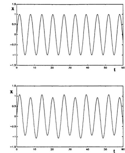
1.7 Time series before and after flip bifurcation. 45

1.8 Characteristic multipliers and phase portrait for flip bifurcation. 46

1.9 Example o f period doubling cascade. 47

1.10 Characteristic multipliers and phase portrait for fold bifurcation. 48 1.11 Characteristic multipliers and phase portrait for Hopf bifurcation. 49

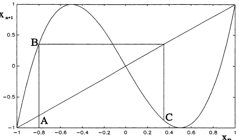
1.12 Graphical iteration o f the cubic map. 50

1.13 Graphs o f x^+2 — around super-critical pitchfork bifurcation. 51

1.14 Super-critical pitchfork bifurcation. 52

1.15 Sub-critical pitchfork bifurcation. 52

1.16 Graphs o f JC„ + 2 = around symmetry breaking bifurcation. 53

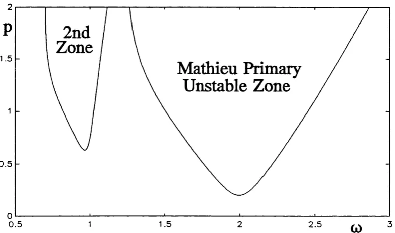
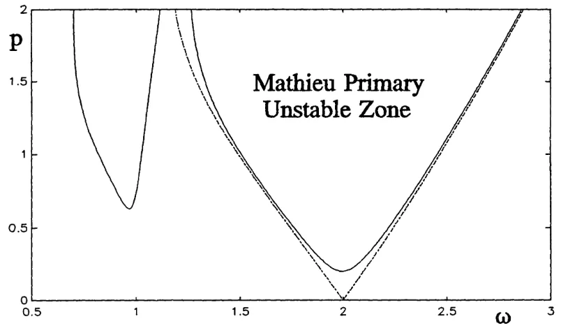
2.1 Analytically calculated boundary to primary Mathieu zone. 63 2 .2 Numerically calculated 1st and 2nd unstable zones. 64 2 .3 Comparison between numerically and analytically calculated zone. 65

3.1 Bifurcation diagram for parametrically excited pendulum. 80

3.2 Locus o f symmetry breaking bifurcation. 81

3.3 Approximation to symmetry breaking bifurcation. 82

3.4 Phase portrait for the undamped unforced pendulum. 82

3.5 Approximate escape locus. 83

3 .6 Time history o f strange attractor. 83

3 .7 Poincaré section o f half o f strange attractor. 84

3.8 Destroyer saddle. 84

3.9 Bifurcation diagram for parametrically damped system. 85

3.10 Integrity curves. 86

3.11a Stable manifolds o f hill-top saddles. 87

3.11b Safe basin. 87

3.12 Heteroclinic tangency. 88

3.13 Bifurcation diagram for parametrically excited pendulum. 89

3.14 Invariant manifolds. 90

4.1 Analytical approximation to upper stability boundary. 97 4.2 Analytical approximation to upper stability boundary. 98

4.3 Schematic bifurcation diagram. 99

5.1 Phase portraits o f rotating orbits. 105

5.2 Bifurcation diagram for rotating orbits. 106

5.3 One quarter o f Poincaré section for rotating chaos. 107

5.4 Bifurcation diagram for rotating orbits. 108

6.1 Poincaré section o f tumbling chaos. 112

6.2 Divergence o f initial conditions. 113

6.3 Largest Lyapunov exponent. 114

6.4 Total angular displacement plots. 115

7.1 Braid diagram formed from time history. 139

7.2 Period-4 knot. 140

7.3 Link diagram. 141

7.4 Reidemeister moves. 142

7.5 Crossings sliding past each other. 143

7.6 Reduced Burau matrices. 143

7 .7 Torus knots. 144

7.8 Decomposition o f reducible orbit. 144

7.9 Moduli o f eigenvalues. 145

7.10 Cubic map with two turning points. 146

7.11 Cubic map with period-3 orbit. 146

7.12 Action o f the cubic map. 147

7.13 Symbolic tree structure. 147

7.14 Spiral 3-shoe. 147

7.15 Homoclinic tangle. 148

7.16 Homoclinic tangle with main pips. 148

7.17 Schematic homoclinic tangle. 150

8.1 Idealised 3-shoe. 169

8.2 Location o f period-3 orbit in 3-shoe. 169

8.3 Location o f period-3 orbit in trellis. 170

8.4 Location o f period-3 orbit in escape zone. 171

8 .5 3-shoe operations. 172

8 .6 Period-2 bifurcational subform. 172

8 .7 Period-3 period doubling cascade. 173

8.8 Pseudo Anosov orbit. 173

8.9 Moduli o f eigenvalues. 174

9.1 Period-2 orbit and close recurrent trajectory. 183

9.2 Some unstable rotating orbits. 184

9.3 Framed braid. 185

List of Tables

8.1 Crossings matrix for period-1 and period-2 orbits. 175

8.2 Crossings matrix for all period-3 orbits. 176

8.3 Word length for orbits up to period-7. 176

8.4 Alexander polynomials. 177

8.5 Orbit classification. 177

8.6 Topological entropy. 178

8.7 Linking numbers o f implied orbits. 178

After familiarising the reader with the analytical and numerical techniques applied in the ! following chapters we begin a systematic analysis of the various categories of the

I

|- pendulum motion. In chapter 2, the hanging solution is considered in terms of stability,

j

Chapter 1: Introduction

The parametrically excited pendulum o f figure 1.1, a simple vertically forced rigid pendulum constrained to move in the plane is a paradigm for nonlinear systems in that despite its apparent simplicity, a wide range o f possible solutions and bifurcational behaviour can be realised over a moderate range o f operating parameters. The system can also be used as a physical demonstration [Leven et al. 1985] to give a convincing visual display o f many nonlinear phenomena, including chaos. As well as the obvious mathematical attraction to studying the parametrically excited pendulum [Mawhin 1988], there is a strong interest to study this system within the engineering community, as the pendulum is a good rough approximation for many systems, from the behaviour o f off-shore structures [Rainey 1977], crane barges [McCormick and Witz 1993], buildings in earthquakes [Housner 1963], to the response o f Josephson junctions [Salam & Sastry 1985]. In all these applications, despite the obvious simplification in the modelling process, much o f the behaviour o f the system can be characterised at least qualitatively by the parametrically excited pendulum. Other pendulum models that have been studied

& Westervelt

of an even larger class o f systems with symmetric potential energy functions [Clifford & Bishop 1993]. Before we begin a systematic description o f the bifurcational behaviour o f the parametrically excited pendulum, we outline some analytical and numerical techniques used in the following chapters.

1.1 Analytical Techniques

escape to an attractor at infinity. This would make deciding whether a trajectory has escaped considerably easier when numerical integration is applied.

1.2 Numerical Methods

A nonlinear dynamical system can be described by a set o f autonomous first order ordinary differential equations o f the form:

X = f(x), xe'sr (

1

Typically we will consider systems in three dimensions with time periodic forcing, and so equation (1.1) becomes

X = /(jc,ri, where x is a vector.

Solutions to equation 1.2 can be calculated relatively easily by a numerical integration technique such as a high order Runge-Kutta algorithm. The inputs are the initial condition vector Xq, and starting time Iq. The behaviour is computed by calculating x

1.3 The Poincaré Map

The stroboscopic Poincaré section is defined as an n-1 dimensional hypersurface transversal to the flow in the n dimensional space spanned by x [Guckenheimer & Holmes 1983]. This is obtained simply by sampling the flow at t mod T = 0. A solution can then be described by the series o f points at which the flow intersects the Poincaré section, a,-, a,+2, ... where = PiaJ, and P(x)

is the Poincaré map. This reduction o f an « dimensional flow to an « -/ dimension map allows the same phenomena and problems o f the qualitative theory o f ordinary differential equations to be studied in their simplest forms [Smale 1967]. A mapping may also be called a diffeomorphism. The Poincaré map can be computed numerically by

integrating equation (1.2) between t = 0 and T in an integer number o f steps.

1.4 Attractors

1.4.1 Fixed Point

A fix ed point is an attracting point in phase space. That is, all nearby trajectories will settle on to the fixed point. The classic example o f a fixed point is the hanging solution o f a simple damped pendulum. Any initial condition will produce a trajectory which decays to this hanging solution as time increases. The rate at which the oscillations die away will depend on the damping present.

1.4.2 Limit Cycle

If we introduce a small periodic horizontal force to the simple damped pendulum, we expect the pendulum to oscillate periodically. This is an example o f a limit cycle, or periodic attractor. Taking a Poincaré section after the transient behaviour has died away will yield a number o f points. If there is only one point, then the period o f oscillation is identical to the period o f the forcing - hence we have a period-1 attractor. If, however there are p points in the Poincaré section, then the period o f oscillation is p times the period o f the forcing. Hence we call the solution a period-p attractor or limit cycle. Limit cycles with p > l 2x t sometimes called

1.4.3 Torus

If a system responds at an incommensurate frequency to the forcing frequency we will see a series o f dots on the Poincaré map winding around a circle. Such

the dimension,

behaviour requires n > 4 and will not be o f further interest here, as the systems we consider have n < 3 .

1.4.4 Chaos

attractor, we may be able to produce some bounds on the behaviour. Another feature o f a chaotic system is that short portions o f the time series may appear to be nearly periodic as the chaotic attractor contains many unstable periodic orbits [Eckmann & Ruelle 1985]. We will see how this property can be exploited in chapter 9.

1.5 Basins of Attraction

Given that a nonlinear system may possess more than one attractor, we need to have some measure o f the relative importance o f each attractor in terms o f how likely we are to achieve each solution. The set o f all initial conditions which lead to an attractor i is termed the basin o f attraction. Various measures have been proposed to measure the area o f a basin [Soliman & Thompson 1989, McRobie & Thompson

1991, Schiehlen 1993], and will be discussed further in chapter 3.

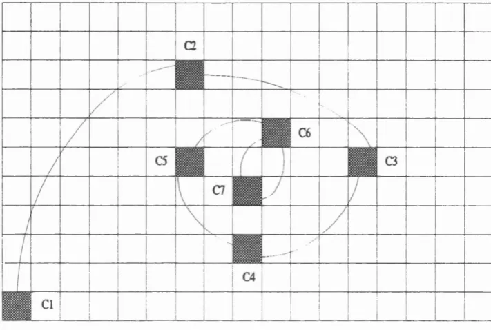
non-empty cell is visited. If the new cell is in the string o f cells encountered, then we have located a limit cycle. The period o f this limit cycle can be calculated by the number o f iterations it takes to return to this cell. All cells C l, C2, ... are labelled as being in the basin o f attraction o f this new attractor, i Alternatively,

we have landed in a cell which has already been identified as being in the basin o f another attractor that has previously been located. If this is the case, the cells C l, C2, ... are labelled as belonging to this attractor. The method has been earned out , and by colouring in the basins o f different attractors accordingly, figures such as

are produced

figure 1.4, where the basins o f three competing attractors are shaded accordingly.

1.6 Locating Solutions

If we define the residual map GfXo) as

G(V =

- *0

we require the solution

G(X

) = 0

(1.5)

Differentiating equation (1.4) with respect to initial condition, Xo gives:

DG(x^ = D P ’’(x^ - I

0

0

DP"(Xq}, the Jacobian [Thompson & Stewart 1986] o f the Poincaré map can be

calculated by either a simple finite difference method, or by variational equations. If we write

and differentiate with respect to initial condition Xq, we have:

D J = D J ( x ) D x (

1

8

4) ^

Define:

X = D x (

1

9

X = D J ( x ) X

(1.10)

D /(x ) can be written in full as:

m x f ) = dx,

% %

âXj ax.

(1.11)

and so by numerically integrating the Jacobian with initial conditions I, we can calculate DP"(a).

Using the Newton-Raphson root finding method, a better estimate o f the fixed point o f the map is given by:

= a. - [D G {a)Y^ G (a )

(1.12)

1.7 Unstable Fixed Points

We have already indicated that the Newton-Raphson method can locate unstable solutions. An unstable solution is a steady state solution which a typical trajectory will depart from exponentially with time. For example, the simple damped unforced pendulum could be balance upside down, but any small perturbation would result in the pendulum toppling over. There are unstable limit cycles, unstable tori, and even unstable chaotic attractors. The stability o f a particular solution x(t) = x^it) can be assessed in terms o f the moduli o f the eigenvalues o f the derivative matrix:

dx^

obCj âX j

(1.14)

If any o f the moduli o f the eigenvalues are greater than 1, then the solution is unstable, whilst a stable solution has all its eigenvalues contained inside the unit circle [Thompson & Stewart 1986]. The case o f a fixed point with eigenvalues both inside and outside the unit circle is a saddle cycle.

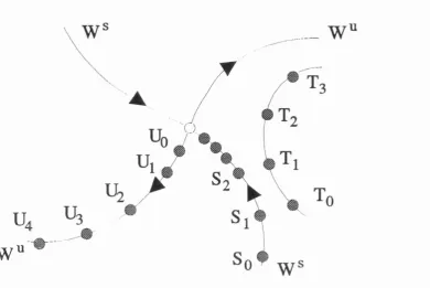
asymptotically by mapping along the points Sj. Conversely, the point Uq is mapped away from the saddle along the unstable manifold. It is important to note that the stable and unstable manifolds are not trajectories, but the set o f all points in the map which approach or leave the saddle asymptotically under the action o f the mapping function. For this reason, the stable manifold is also known as the inset, and the unstable manifold as the outset.

1.7.1 Importance of Unstable Solutions

At first glance, unstable solutions are unimportant to engineers; they are not attracting solutions, and so are not observed as solutions in real systems. However, unstable solutions are o f vital importance for many reasons. Firstly, the unstable manifolds o f saddles can form the boundaries between competing attractors. We have seen already the importance o f calculating basin boundaries. Unstable solutions can be controlled by simple modem control techniques [Shinbrot et al. 1993], and by carefully choosing an unstable solution, the performance o f a given system may be enhanced in some measurable way. Also, the unstable solutions form a skeleton around which trajectories wind [Artuso et al. 1990a,b], and by describing a few unstable solutions, the nonlinear system may be characterised and completely understood [Mindlin et al. 1990]. These startling claims will be expanded in chapter 7. Unstable solutions can also be followed as the parameters o f a system are changed,

at bifurcations

1.8 Path Following

As the parameters governing the behaviour o f a system are allowed to vary, the solutions will generally evolve slowly except at bifurcations [Thompson & Stewart 1986]. A particular solution or fixed point o f the Poincaré map can be followed by continuously applying the Newton-Raphson scheme at every small change in the parameter. However, the technique is further improved bypredicting how the solution will evolve. This is achieved by redefining the residual map to include the variation o f a parameter, a. Equation (1.14) becomes

cbCj

% % %

=

(1.15)

1.9 Bifurcational Behaviour

We have already seen that a nonlinear dynamical system can often be modelled (section 1.2) in terms o f a low dimensional ordinary differential equation. Typically three dimensions are enough to characterise a large amount o f the behaviour found in higher dynamical systems. Often in these systems we are concerned with qualitative changes o f behaviour in the system due to the variation o f a control parameter or parameters . This may be achieved by studying the bifurcational behaviour [Abraham & Shaw 1988]. The term bifurcation refers to the branching o f one path o f equilibrium to an alternate qualitatively different path or paths by varying a control parameter [Guckenheimer & Holmes 1983]. Bifurcation theory is vital to the understanding o f nonlinear dynamical systems, and here the bifurcations are considered by varying one control parameter only. These are known as codimension one bifurcations. Further bifurcations are possible with the control o f two or more parameters.

Consider the ordinary differential equation:

Jc + c i + ax^ = Fit) (1*16)

i l = ^2 = /iW

= F(t)

- cxj -

(1-17)

f = 1

Solutions o f equation (1.17) can be located by the variety o f numerical and analytical techniques considered earlier, and the stability o f a particular solution x(t) = Xq(1) can

be assessed in terms o f the moduli o f the eigenvalues o f the Jacobian. As the control parameter is varied, the eigenvalues or characteristic multipliers change, and one may leave the unit circle at a bifurcation. The type o f bifurcation produced depends crucially on where the characteristic multiplier leaves the unit circle, and the other solutions in the vicinity o f the bifurcating solution. Some typical bifurcations that occur in the systems we shall be interested in are considered below.

1.9.1 Flip Bifurcation

see that at the bifurcation, a characteristic multiplier leaves the unit circle through -1. The old period 1 limit cycle becomes a saddle cycle, and since a typically close trajectory will oscillate about this saddle cycle it is an inverting or I-type saddle, A period-doubling bifurcation o f a period T to a period 2T limit cycle may be followed by another period-doubling to a period 4T limit cycle and so on. This cascade o f bifurcations has been studied by Feigenbaum [Feigenbaum 1980], and often occurs in nonlinear systems. A period-doubling cascade is shown in figure 1.9.

1.9.2 Fold Bifurcation

solutions, so trajectories wander out o f the section to a distant stable limit cycle, or go to infinity.

1.9.3 Hopf Bifurcation

1.9.4 Symmetric Bifurcations

Symmetric systems possess at least three additional codimension 1 bifurcations. Whilst some may argue that symmetry is somehow nongeneric, this is not a view shared with nature, and strong evidence exists o f symmetric bifurcations in experimental systems [Stewart & Golubitsky 1993, Mullin 1993]. To study symmetric bifurcations, consider the difference equation:

with X defined over the interval [-1, + 1 ]. Just as integrating a second order ordinary differential equation over one period o f forcing produced a two dimensional mapping, equation (1.18) represents a one dimensional map o f the interval [-1 4-1] to itself under the mapping:

The iteration o f a one dimensional map can be carried out graphically as in figure 1.12. We start at point A with = -0.8, and take a line up to point B and read o ff Xj = 0.352, next take a horizontal line across to the dotted line = x„, and then vertically down to point C = -0.88154, and so on.

1.9.4.1 Super-critical Pitchfork Bifurcation

The cubic map equation (1.18) [Mullin 1993] has an obvious period-1 solution

X = 0. The stability o f this solution can be considered by evaluating the derivative at jc = 0.

Æ . dx_

=

3ax^ + l - a = l - a

(1.20)

x . = 0

period 2 solutions can be calculated by putting x„+j = into equation (1.18). After some manipulation we discard the trivial zero solution to be left with:

We see immediately that this solution is only possible for a > 2 , the value already obtained for the super-critical pitchfork bifurcation.

1.9.4.2 Sub-critical Pitchfork Bifurcation

A catastrophic bifurcation for symmetric systems may be obtained by swapping the stable and unstable solutions from the super-critical pitchfork bifurcation to give the scenario displayed in figure 1.15. Here an unstable symmetric period-2 solution collapses around the stable zero solution to leave only the unstable zero solution. This is termed a sub-critical pitchfork bifurcation.

1.9.4.3 Symmetry Breaking Bifurcation

dx^

dF^ dx

ÊL dx

_ dF dx

X - - S

2

dx

(1.22)

Hence the second derivative must always be positive, ruling out a flip bifurcation to a symmetric period 4 solution. The only way to lose stability is for the second derivative to equal + 1 . The value o f alpha for this bifurcation can be calculated from equation (1.21).

'd F dx

= 1

(1.23)

(2a - 5)^ = 1

a = 3

Plotting the graph o f against around the bifurcation value in figure 1.16 shows that the unstable symmetric period two solution, S has produced two stable ‘mirror image’ period two solutions, A and B. This is termed a symmetry breaking

since the stable symmetric solution is destroyed

1.9,5 Bifurcation Following

Bifurcations can be followed in parameter space by adding the constraint that one o f the eigenvalues o f the Jacobian lis 4-1, -1, or o f modulus 1 for the respective

(see section 1.6)

bifurcations considered. The variational method cannot be used in this case and so we must resort to the finite difference method [Foale & Thompson 1991].

1.9.6 Global Bifurcations

1.9.6.1 Heteroclinic Saddle Connection

A heteroclinic saddle connection can cause the basins o f attraction o f competing attractors to be suddenly altered. This is shown in figure 1.18. There are three competing attractors (not shown in the figure), with basins hatched accordingly. The grey basin is unaffected by the sequence o f events leading up to the saddle connection, whilst the other two basins are dramatically altered by this event. Since the bifurcation only causes the basins o f attraction to be altered as opposed to the nature o f any attractor, the event is called a basin bifurcation [Abraham & Shaw

1988].

1.9.6.2 Homoclinîc Saddle Connection

large basin may be instantaneously destroyed leaving no attractor. Hence this is a catastrophic bifurcation.

1.10 Nonlinear Dynamical Systems - a Numerical Approach

We have developed the necessary tools for analysing the behaviour o f nonlinear dynamical systems expressed as ordinary differential equations. These tools, when used carefully and systematically can provide an understanding o f complex nonlinear phenomena. Here we outline the approach advocated by many dynamicists:

1) Carry out a cell mapping algorithm on a region o f phase space that is likely to contain the relevant attractors. Repeat at various parameter values to locate stable solutions.

2) Given the stable solutions located by step 1, path follow these solutions through parameter space to produce typical response curves. Note any bifurcations encountered in path following.

3) Follow the bifurcations by adding the eigenvalue constraint to the minimisation process and produce a bifurcation diagram.

4) Carry out further cell mappings at parameter values that are relatively unexplored to locate additional attractors, and proceed as before.

Figures for Chapter 1

\ J

\

\

\

m

Figure 1.1: The Parametrically excited pendulum, mass m, length 1, subject to periodic displacement z(t), and constrained to move in the plane.

— 3

1 O 20 30 70 SO

U , w "

0

- 1

- 2

- 3

3

- 2 - 1 0 1 2 4

X

t

X

;

Im

A

^

V"

. .—-Il

<:

's.

% 1

;

Im

Re

1 - '

o

Ln

r 'A

A

A

\

A. "Ao

V,.

y

V,„

_{A, . >}

n+1

0 .5

- 0.5

- 1

- 0.8 - 0 .6 - 0 .4 0 0.2 0 . 4 0.6

- 1 - 0.2 0.8

0 .5

-0 .5

-0.8 - 0 4 -0 .2 0 0.2 0 .4 0 .6 0.8 1

1 -0.6

X

0 .5

-0 .5

-0 .4 -0 .2 0 0 .2 0.4 0.6 0.8 I

- 1 -0 .8 -0 . 6

X

■n+2

0 .5

-0 .5

-0.2 0 0.2 0 .4 0.6 0.8

1 -0.8 -0.6 -0 .4

Figure 1.13: Graphs ofx„+2=^« for a = 1.9, 2, 2,1 around the super-critical pitchfork

— 0.5

-1 . 2 1 .e 1 .8 2 2.2 2 . 6

Figure 1.14: Super-critical pitchfork bifurcation for the cubic map. The solution %=0 is stable for a < 2 , and unstable for œ > 2 . A period-2 stable symmetric solution exists for o! >2.

0.6 0.4.

0.2

- 0.2

-0.4

- 0.6

n+2

0 .5

-0 .5

—0.8

1 -0 .6 -0 .4 -0.2 0 0 . 2 0 .4 0.6 0.8 I

Xn

0 .5

-0 .5

0 .8

- 1 -0.8 -0.6 -0 .4 -0 .2 0 0.2 0 .4 0.6

X

0 .5

-0 .5

-0.2 0.8

1 -0.8 -0 .6 -0 .4 0 0.2 0 .4 0 .6

X

0 .5

- 0 .5

- 1

2.5 3 3.5

1 1.5 2

) •

Figure 1.18: Heteroclinic saddle basin bifurcation. Two o f the three shaded basins o f attraction change as the heteroclinic saddle connection is broken. Since there is no change in the attractors, this is called a basin bifurcation.

Chapter 2: Parametrically Excited Pendulum: Hanging Solution

The equation o f motion o f the parametrically excited pendulum can be written as:

f-Q " + É .Q ' + H i " + g)sin0 = 0 (2.1)

m

(see figure 1.1).

where the pendulum subject to periodic displacement z(r) is o f length 1, mass m, and has linear damping d, where a dash denotes differentiation with respect to time, t. By writing:

Z(t) = -ZcO SQ t , t = CD^jT , (Oq = 8

(2.2)

equation (2.1) reduces to

0 + c6 + (1 + pcosa)r)sin6 = 0

where:

c , p - , 0) - — (2.4)

whether this solution is stable in the sense that a small perturbation from the hanging position will produce damped oscillations back to the zero solution, or be magnified. This can be predicted by a linearisation about 0 = 0 . Noting that for small 6,

sin 0 = 0 -0^/31 + ...

we take thei first erm in the expansion to get the approximate expression:

0 + C6 + (1 + /7COSG)f)0 = 0

Re-scaling time according to T=wf/2, and differentiating with respect to t gives:

0/' + ^ 0 ' +

0)

c o s2t

0 = 0

(2.6)

For c = 0 , this reduces to the same form as the Mathieu equation as studied by a number o f researchers [Jordan & Smith 1987, Hayashi 1964]:

M + (Ô + 2eco s2 t)u = 0

(2.7)

where

6 = A (2.8)

and

2.1 Method of Strained Parameters

We assume that e is a small parameter, and expand w as a function o f time, t and e, and also expand 6 as a function o f e alone.

M(f,e) = Mq(0 + + .... (2.10)

Ô = Ôq + eô j + + .... (2.11)

The two expressions are substituted into equation (2.9), and we equate like powers o f e.

e®: = 0

e^: + ÔqMj = -ÔjMq - lu ^ c o slt (2.12) ef: « 2 &o%2 " “ 2u^cos2t

For the largest zone of instability, we put = 1, and solve equation (2.12a) to get:

M

= acosf + 6sin^

(2.13)

(

2

12

substituting the initial solution into gives:

Mj + Wj = -ôj(acosf + Z>sinf) - 2(acosf + 6sinf)cos2f

Any terms in cos(t) or sin(t) on the right o f the equation (2.14) are called secular terms, and if any non-zero secular terms exist then the solution to equation (2.14) will increase exponentially with time. To eliminate secular terms, we have two possibilities:

ôj = - 1 6 = 0

ôj = +1 a = 0 (2.15)

This leaves:

+ Mj = - ( a c o s 3 t + 6sin 3f) (2.16)

Taking the first case, 6 = 0 gives:

K. = — cos3f (2.17)

^ 8

% substituting (2.17) into equation (2.13) we get:

cosf + —cos3f - —cos5r (2.18)

Taking the alternative case, a = 0 gives:

M, = — sin3r

^ 8

(2.20)

by substituting into equation (2.13) we get:

«2 + «2 = - b

r- • i)

sinr + — sm3f - — sin5f

8 8

(2 .21)

Again, for no secular terms, we require the coefficient o f sin(t) to be zero, so:

(2.22)

Hence, the two periodic solutions that separate the stable and unstable behaviour o f the zero solution are described by:

0 = 1 ± € - — + O(e^) 8

(2.23)

Substituting the original variables gives a quadratic equation in w^:

unstable zones exist around w = 1, 3/4, 1/2, 1/4, and so on.

2.2 Numerical Computation of Unstable Zones

The unstable zones for the parametrically excited pendulum can be calculated numerically by assessing the stability o f the zero solution in terms o f the eigenvalues o f the Jacobian. By adding the eigenvalue constraint, and bifurcation following, the numerically

exact unstable zones are shown in figure 2.2 and compared with the analytical approximation in figure 2.3. The effect o f the nonzero damping is to lift the primary unstable zone away from the x-axis, and to shrink other unstable zones. This makes the primary unstable zone the most important zone in terms o f its influence over a large parameter range.

2.3 Effect of Higher Order Terms

Figures for Chapter 2

Mathieu Primary

Unstable Zone

0 . 5

1.5

0 . 5 1 2 2. 5

0 3

2nd

Zone

Mathieu Primary

Unstable Zone

0 . 5

1.5 3

0 . 5 1 2 2. 5

(0

Mathieu Primary

Unstable Zone

0 . 5

3

2 2. 5

1.5

0 . 5 1

CO

Chapter 3: Parametrically Excited Pendulum:

Non-Rotating Solutions

In many applications o f the parametrically excited pendulum, the main interest going beyond this value is in achieving solutions that do not exceed 6 = ±tt, as might correspond to failure in some sense. We term such solutions non-rotating, for the obvious reason that the pendulum does not rotate completely about its pivot point, but just oscillates back and forth. It is useful to develop a method which can predict which parameter zones will inevitably lead to solutions which go ‘over the top’ after a finite number o f cycles o f applied parametric excitation. Such parameter regimes are termed ‘escape zones’. This can be achieved by both analytical and numerical techniques. Under the conditions expressed, we have an ‘escape’ problem. Such a problem is common in

the

by the ^ numerical, techniques outlined in chapter 1.

3.1 Bifurcational Behaviour

d= ± T r after a finite number o f periods o f applied parametric forcing. The features o f the bifurcation diagram agree with those produced by Mullin [Mullin 1993], and Bryant and Miles [Bryant & Miles 1990c].

The bifurcation diagram figure 3.1 for non-rotating orbits in the parametrically with

excited pendulum is very similar that produced by Soliman and Thompson for escape from an asymmetric potential well under parametric excitation [Soliman & Thompson 1992a,b] except o f course for the symmetry breaking bifurcation which is not applicable. There is also considerable similarity to the bifurcation diagram for escape from an asymmetric potential well under direct excitation [Thompson 1989], except again for the symmetry breaking bifurcation, and additionally the super-critical pitchfork bifurcation, which does not occur.

3.2 Analytical Solution: Harmonic Balance

Following Capecchi and Bishop [Capecchi & Bishop 1994], we assume a solution o f the form:

^ - [p(7,(A) - y,(X ))c(«p cos8q + 2 7 i(4 )co seo ] = 0 (3.2a)

Ci4o> - l\p{J^ (A ) + J3(A ))sinPcos0J = 0 (3.2b)

sm8Q[p.^(/4)cosp - Jq(A)] = 0 (3.2c)

of the first kind

where J„(x) is the Bessel function ot order n. These three simultaneous equations could be solved numerically to give an approximate analytical solution by a

Newton-information

Raphson technique. However, more can be derived by considering the various solutions that are known to exist.

Equation (3.2c) can be split further into:

sin 0Q = 0 (3.3a)

symmetric solution

or p J2(A )cosp - Jq(A) = 0 (3.3b)

asymmetric solution

For the symmetric solution 6q = 0, equations (3.2a,b) reduce to:

_ ^ ^

-

(3.5)

J , ( 4 ) *

y,(X)

In the case o f asymmetric solutions, for c = 0; /8 = 0 and for light damping c » 0 « 0, so equation (3.4) becomes:

pJ^(A) - Jg(X) = 0 (3.6)

3.2.1 Bifurcation Criteria

procedure to give the parameters where both symmetric and anti-symmetric solutions exist in the (w,p) plane; i.e. the locus o f the symmetry breaking bifurcation. The results are good for w > 1.5, but poor at low frequency when compared to the locus obtained by a bifurcation following technique. This is shown in figure 3.2 where the approximate analytic solution is compared with the numerically computed symmetry breaking bifurcation.

The sub-critical bifurcation can be determined by the usual vertical tangency condition:

^ ~ (3.7)

d<ù

This occurs at A = 0, and so by differentiating and taking the limit as A -» 0, equation (3.4) yields:

[o)^ - 4 f + 4c^g)^ - 4p^ = 0 (3.8)

which agrees with the result obtained in chapter 2 by analysing the linearised form o f equation (2.1); the Mathieu equation. Hence, equation (3.8) gives a good approximation to the left hand boundary o f the escape zone.

3.2.2 Critical Velocity Criteria

Another approximate criteria for escape is that proposed by Moon [Moon 1987], that escape/chaos occurs when the maximum velocity o f the motion is near the maximum velocity on the separatrix, (that is the stable or unstable manifold which

I trajectories and solutions

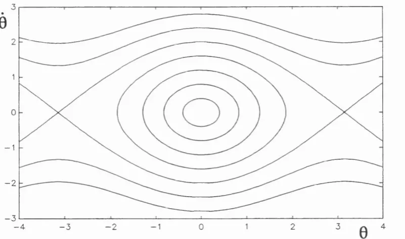
forms the basin boundary between escaping — vhich remain in the potential well) for the phase plane o f the undamped, unforced oscillator. For the undamped, unforced pendulum, the phase plane shown in figure 3.4 is composed o f concentric ellipses and rotating orbits.

The maximum velocity on the separatrix is:

L - 2

(3.9)

From the harmonic balance solution;

0(f) = -i4va)sin(o)f + P)v

(3.10)

*■

Ù)

(3.11)

Truncating the Bessel functions and averaging equation (3.4) gives [Capecchi & Bishop 1994]:

[ i î ! - 2 +

= 0

(3.13)

2

4

12

where

- ^ c (1-^ /6)

(3.14)

(l-^ " /1 2 )

substituting equation (3.12) into equation (3.13) gives;

= (fa)^ - 4(0^ + S a y + 4 w 9 4 (w : - i f ) :

For low damping;

^ 3(w" - 4w : + 8g:)

(3.16)

2(3o>: -

\ denoted by M

The curve obtained from the approximation equation (3.16) is plotted in figure

lis

The two analytical methods employed to give approximations to the escape zone both yield reasonable results. The bifurcation criteria method is the more accurate especially at high frequency, but the critical velocity criteria does have the advantage o f producing a closed form analytical expression for the zone rather than needing to solve a series o f nonlinear equations numerically. Whilst both methods give good results, it is also worth noting that although stable non-rotating solutions exist below the escape zone, their basins o f attraction may be fractal, and subject to rapid basin erosion, a possibility that we investigate further in section 3.5.

3.3 Chaotic Blue Sky Catastrophe

The bifurcation at the end of the period-doubling cascades is termed a chaotic blue sky catastrophe [Abraham & Shaw 1988]. This is because the two chaotic attractors vanish instantaneously along with their basins of attraction into the blue, leaving no stable non-rotating solutions. 'he chaotic nature o f the attractor is unclear from simply observing

1983]. For example, in the escape from an asymmetric potential well, a period-6 unstable solution has been identified which is responsible for the disappearance o f the final chaotic attractor [Stewart 1987]. Given that there are similarities in the parametrically excited pendulum and the escape from a potential well we hypothesise that a period-12 unstable solution may be responsible for the final event. We choose period-12 rather than period-6 since the fundamental solution which comes from the equilibrium solution is in this case o f period-2, rather than period-1 in the case o f escape from an asymmetric potential well under direct excitation. A Newton-Raphson approach was used around the boundary o f the chaotic attractor, and indeed an unstable period-12 orbit was successfully located. As the forcing parameter is increased the unstable solution was path followed, and found to move closer to the chaotic attractor. This is shown in figure 3.8, where the unstable orbit is seen to collide with the chaotic attractor at a parameter value which is indistinguishable from that o f the final event.

3.4 Generic Features of Escape from a Symmetric Potential Well

under Parametric Excitation

We have already seen that the parametrically excited pendulum has many similarities with other escape systems. Indeed from a series o f detailed observations o f other escape systems, it seems that the parametrically excited pendulum is a typical example o f any system which permits escape from a symmetric potential well under parametrically excitation [Clifford & Bishop 1993]. The reason for this generic behaviour will be shown in section 3.6. Here^we consider a parametrically damped system described by equation (3.17).

X + (1 + ^cosQr)i

(3.17)

relevance to any system which permits escape from a symmetric potential well under parametric excitation.

3.5 Fractal Basin Boundaries

figure 3.10. The window o f 40000 equally spaced initial conditions used \was 6 —±Tr, 6 —± 3 . The basin area is dramatically reduced over a narrow parameter range in the first two cases where the pitchfork bifurcation is sub-critical.

intersections may be important in estimating the final escape o f all trajectories [McRobie 1992c, McRobie & Thompson 1992, 1993a, Yamaguchi & Tanikawa 1992].

3.6 Horseshoe Formation

Figures for Chapter 3

Escape

0. 5

0. 5 1 1.5 2 2. 5

₍₀

/ / / /

0. 5

0. 5 1 1.5 2 2.5 3

1 1.2 1.4 1.6 1.

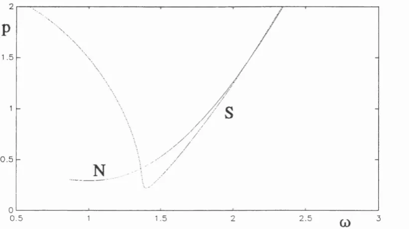
Figure 3.3: Approximations to the symmetry breaking bifurcation, S and the subcritical pitchfork bifurcation, H, obtained by harmonic balance, together with the shaded numerically obtained escape zone for the parametrically excited pendulum.

1 1.2 1.4 1.6 1.8 2 2.2 2. 4 2. 6 2. 8 3

0)

Figure 3.5: Approximate escape locus, M, obtained by critical velocity criteria, together with the shaded numerically obtained escape zone for the parametrically excited pendulum.

-2

- 3

12 14 16 18 20

- 0 . 2 0 4

- 0 . 2 0 6

- 0 . 2 0 8

- 0.2 1

- 0 . 2 1 2

1.45 1.5 1.55 1. 6 1.65

Figure 3.7: Poincaré section of half of strange attractor for the parametrically excited pendulum. Parameters are w =2, p = 1.3426.

- 0 . 2 0 4

- 0 . 2 0 6

- 0 . 2 0 8

- 0 . 2 1

Escape

0 . 5

0 )

1.5

0. 5 2 2. 5 3

60 50

40

30

20

0.4 0.8 1.2

0 0.2 0.6 1

60

50

40

2 0

0.6

0.2 0.4 0.8 1.2 1.4 1 .6

0 1

60

50

40

30

- 1

- 2

- 3

0

- 3 - 2 - 1 1 2 3

Figure 3.11a: Stable manifolds of hill-top saddles for the parametrically excited pendulum. Parameter values areco=2, p = l, c =0 .1 .

- 1

-2

- 3

- 3 - 2 1 0 2 3

- 4 1 4

Zone 2

0 . 5

1.5 2 . 5 3

0 . 5 1 2 ₀₎

-2

- 3

- 3 0

- 4 - 2 1 1 2 3 4

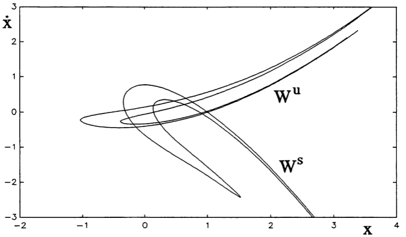
Figure 3.15: Idealised invariant manifolds of figure 3.14,

Wru

Wlu

X

X

Chapter 4: Parametrically Excited Pendulum: Inverted Solutions

It is well known that the inverted position o f the parametrically excited pendulum can be stable for certain values o f forcing amplitude and frequency, as has been demonstrated both numerically and experimentally [Stephenson 1908b, Mullin 1993]. The stable zones can be predicted by linearising the equation o f motion to the Mathieu equation. In addition, there is much in common with the non-rotating orbits discussed in chapter 3.

4.1 Analytical Prediction of Stable Zones

By substituting <t>='jr-6 into equation (2.5), we can describe inverted oscillations by equation (4.1).

^ + c(j) - (I + pcoswf )sin4> - 0

(4.1)

Again, by linearising about <^=0, and re-scaling time, we have a damped Mathieu equation (4.2).

()>// + — <))/ +

(i> ' ± + i£ c o s 2 T '<|) =

0

M + (Ô + 2 e c o s 2 t ) u = 0 (4.3)

where,

G)^ <0^

From the results for the primary Mathieu zone in chapter 2, the boundaries are given by:

0 = 1 ± G - — + O(e^)

(4.5)

8

Substituting equation (4.4) into (4.5) gives a quadratic in cy:

+ (4 ± 2p)(D^ - ^ = 0

(4.6)

4.2 Bifurcational Behaviour

The bifurcations o f the inverted parametrically excited pendulum were determined by path following the unstable solutions located in the vicinity o f the t solution. The solution becomes stable as two mirror image unstable period-1 solutions collide with the unstable hill-top solution. The inverted solution then becomes unstable at a super-critical pitchfork bifurcation, leaving a symmetric period-2 solution. These two bifurcations form the boundaries o f the hatched stable region in figure 4.2.

4.3 Stability of Inverted Pendulums

Figures for Chapter 4

5

P

4

3

2

1

0

0 0 .5 1 1.5 2 2.5 _G) 3

5

P

4

3

2

1

0

2.5 3

0 0 .5 1.5 2 _CO

PI

PI

Chapter 5: Parametrically Excited Pendulum: Rotating Solutions

If we consider the parametrically excited pendulum to have phase space RxSxS by identifying Q—t and 0=-7t, we see that rotating solutions may exist. Firstly we define a rotating orbit as a solution which goes beyond 6 = ±tt. Rotating orbits can be further subdivided into those which rotate in the same direction for all time, that is, ^(t) > 0 vt or 0(t) < 0 Vt, and those which change direction in the course o f their rotation. We call the former solutions ‘purely rotating orbits’, and these will be covered exclusively in this chapter. The orbits which change direction loop around the equilibria ^ = 0 , and 6 —± i r , and can rotate with zero mean angular velocity, i.e. they can return to where they started from without the necessity o f a toroidal phase space. Physically this could correspond to the pendulum performing two clockwise and then two anticlockwise revolutions. To clarify the distinction between rotating and purely rotating orbits, we show phase portraits o f two period-3 orbits in figure 5.1. The first is a purely rotating orbit, whilst the second loops around the equilibrium ^ = 0 before rotating beyond 6=-Tr.

5.1 Analytical Treatment

The harmonic balance procedure applied to non-rotating solutions in section 3.2 can also be applied to the rotating solutions. However, the resulting equations are inseparable, and do not give a very accurate representation o f the behaviour [Capecchi & Bishop 1994]. We avoid using a more accurate higher order harmonic balance procedure as we follow our reasoning in chapter 1 that the strength o f analytical methods lies in their ability to produce a rapid approximate solution. Since in this case this cannot be easily achieved, we resort to numerical analysis.

5.2 Bifurcational Behaviour

explosion, and the trajectories tumble backwards and forwards, rotating clockwise and then anticlockwise in a chaotic fashion which is further investigated in chapter 6. The purely rotating solution restabilises as the tumbling chaos becomes unstable and a very rapid period-doubling cascade in reverse leaves the original (1,1) solution stable in the period-1 zone surrounded by line U.

5.3 Subharmonic Orbits

Figures for Chapter 5

- 1

- 2

- 3

0.2 0 . 4

- 0.6 - 0 . 4 - 0 .2 0 0.6 0.8 1

- 1

6

/tï

- 1

- 2

- 3

- 0.2 0 0.2 0 . 4 0.6 0 .8 - 0.8 - 0 .6 - 0 . 4

- 1

Tumbling

Chaos

2.634

2.632

2.63

2.628

2.626

2.624

2.622

L-0.6 0.62 0.64 0.66 0.68 0.7 0.72 0.74 0.76

Tumbling

Chaos